

Identification of Corrosion on the Inner Walls of Water Pipes Using a VGG Model Incorporating Attentional Mechanisms
Abstract
:1. Introduction
2. Image Acquisition and Sample Set Production
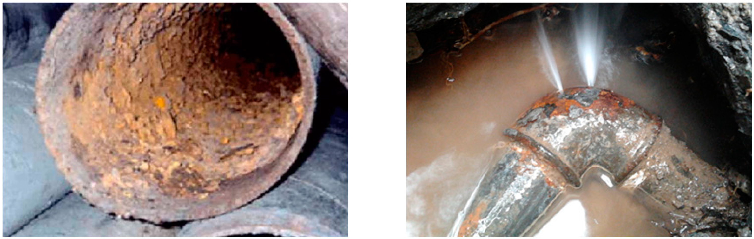
2.1. Pipeline-Damage-Image Acquisition
2.2. Preparation of Experimental Sample Set
3. Method
3.1. Basic Concept of Convolutional Neural Networks
3.2. Mathematical Principle of Convolution Neural Network
- (1)
- Set as the initialization data input to the input layer for the first time, and as the output result of data after convolution operation in the first convolution neural network; is the parameter of the first layer of the neural network. At the same time, is input to the second layer of the network, and is output after convolution and pooling through the second layer of the network; is the parameter of the second layer of the neural network, which is calculated to the last layer of the network in this way, while can be set as its final output result and is the parameter of the last layer network. Finally, to determine differences between the output value and the predicted value and calculate the loss value of the network as , the expression is:
- (2)
- The dimension of the output of the convolutional neural network is the same as the real value , and the expression of the predicted value obtained after forward propagation is:
- (3)
- Set the sample data inputted to the input layer for the th time by the convolutional neural network as . At the same time, set as the weight in each layer of the network, and as its offset in each layer. The output result is . The loss function can be calculated, and its mathematical expression is:
- (4)
- Carry out iterative training many times, and constantly update the parameter weights of the network, so as to minimize the loss function of the network. Next, the calculation method of gradient direction descent is used to conduct systematic learning and design updating for all kinds of weight parameters and offset weight values of the whole network. Let the network weight of the th iteration be and the network offset be . The mathematical expressions of and at this time are calculated as follows:
- (5)
- In the process of forward nerve propagation, is used to directly represent the active activity state of neurons in layer , and is used to represent the active state value of neurons in the first level after activation. Subsequently, the expression of neurons in layer is defined as:
- (6)
- To calculate the partial derivative of the loss function of the layer neural network to the neuron of the layer , recorded as , the mathematical expression is:
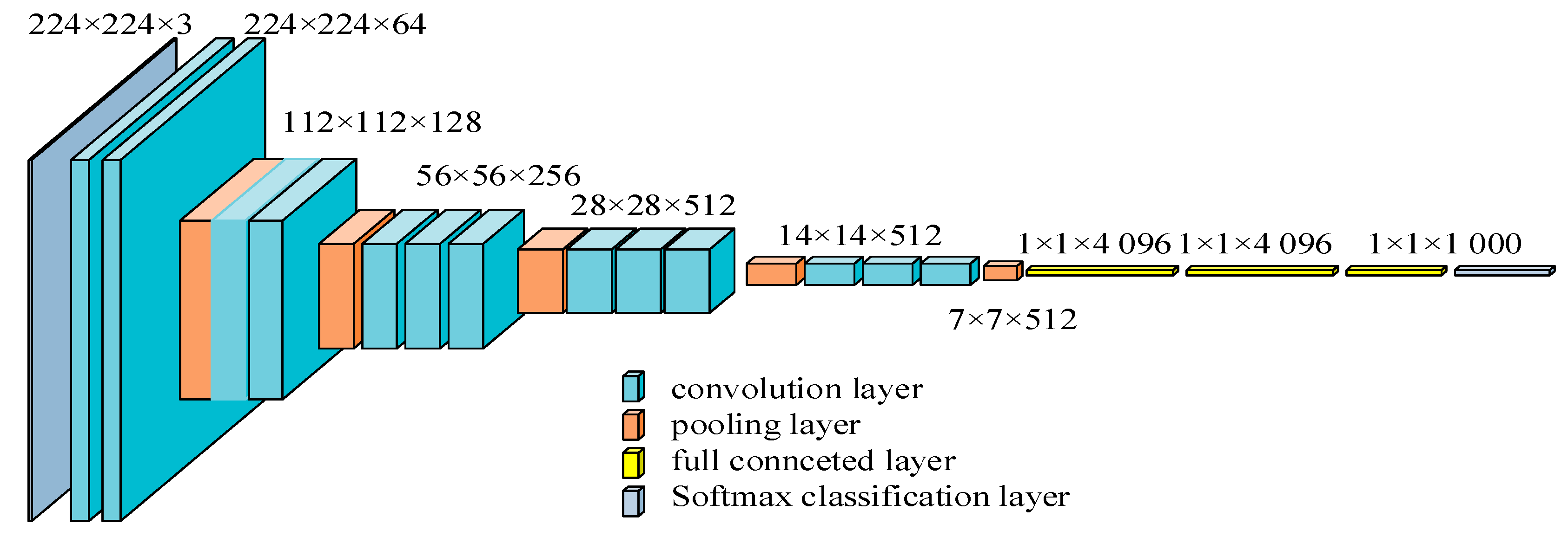
3.3. VGGNet
3.4. S.E. Attention Mechanism
- (1)
- Squeeze () operation: This step pools the image’s feature maps to obtain each channel’s global features, as shown in Equation (13).
- (2)
- Excitation () operation: This step is performed through two fully connected layers that generates the required weight information through the weights, which are obtained through learning and are used to model the relevance of the features needed for the display, as shown in Equation (14).where is the first full-connection-layer operation, is the second full-connection-layer operation, is the activation function Relu, and is the activation function Sigmoid.
- (3)
- Reweigh () operation: The weights obtained in the previous step are weighted to the original features by multiplying them channel by channel to complete rescaling of the original features in the channel dimension, as shown in Equation (15).
3.5. Improved VGG16 Model
3.5.1. SE-VGG16 Classification Model
3.5.2. Multi-Loss Function Fusion
3.6. Hyperparameter Optimization
| Algorithm 1: Labeling Bayesian optimization algorithm |
| Input: Agent model , collection function . |
| Output: Hyperparameter vector . |
| 1: for …., do. |
| 2: Maximize the acquisition function to obtain the next evaluation point: |
| 3: Evaluate the objective function value ; |
| 4: Consolidate data: , and update the probabilistic agent model; |
| 5: End. |
4. Experiments
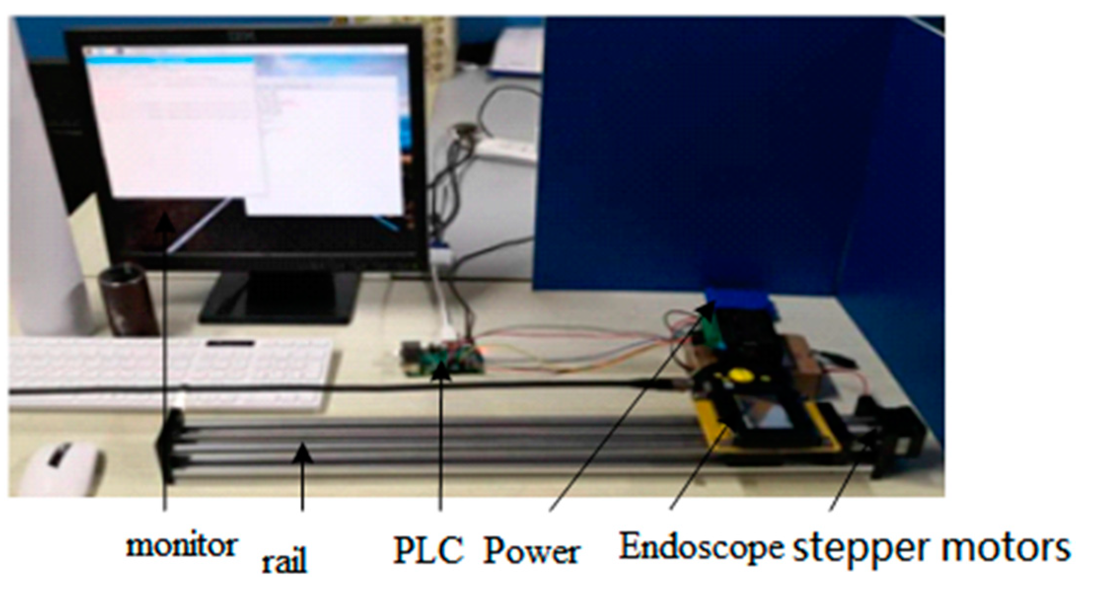
4.1. Experimental Platform
4.2. Model-Parameter Setting
4.3. Comparison and Analysis of Experimental Results
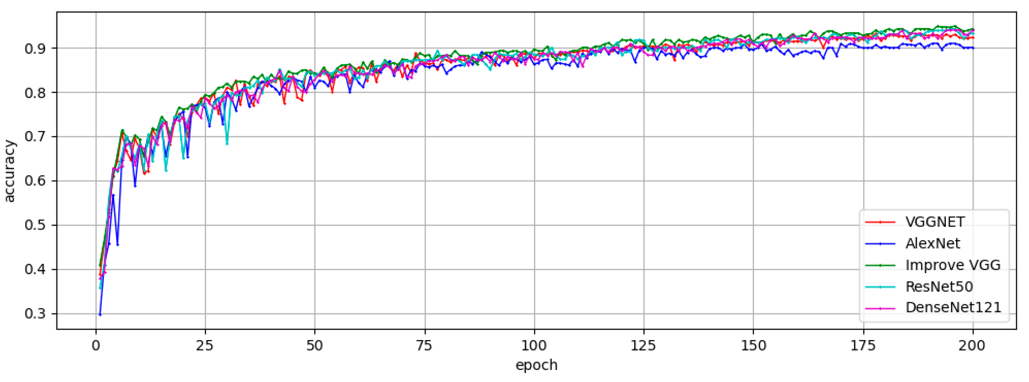
4.3.1. Comparison of Model Training Results
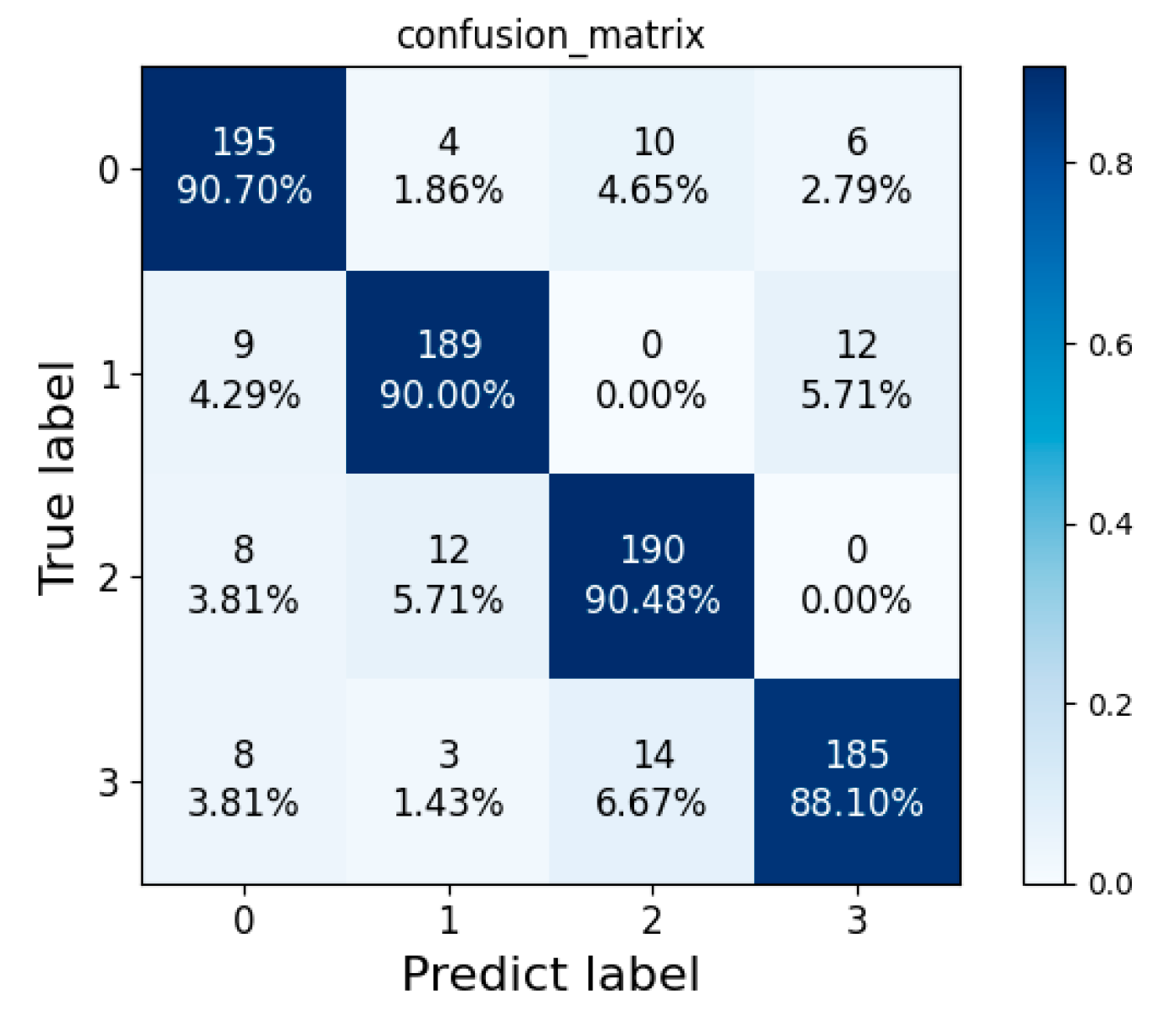
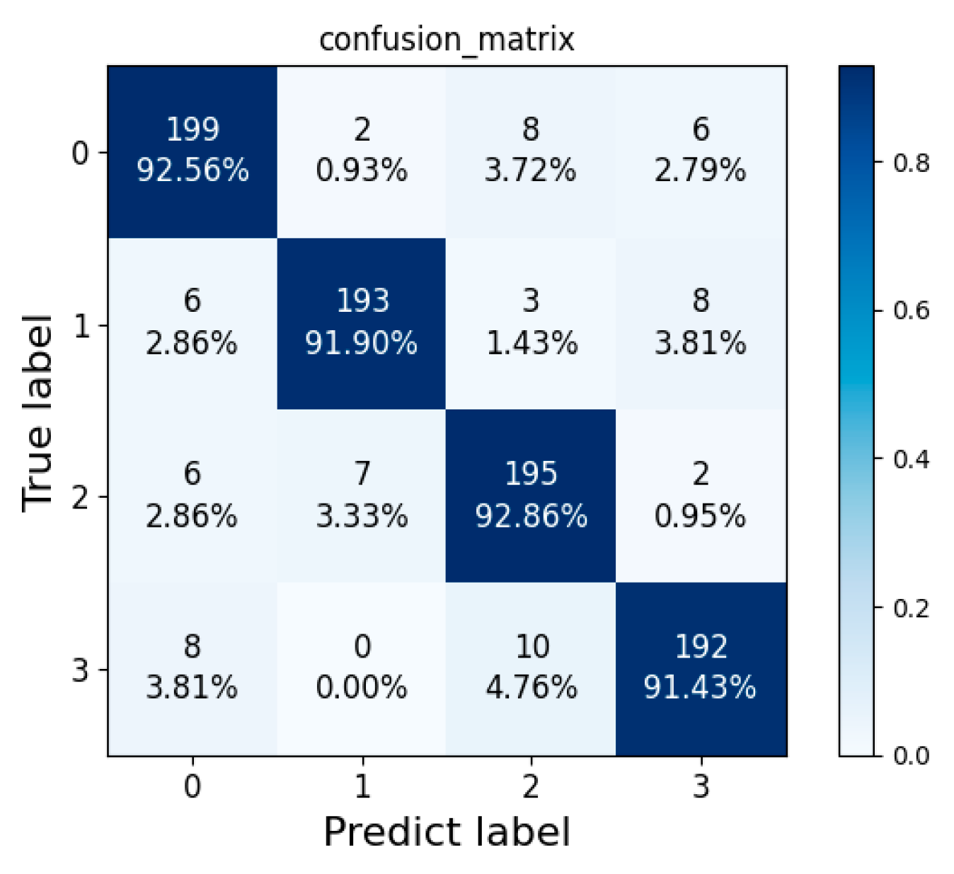
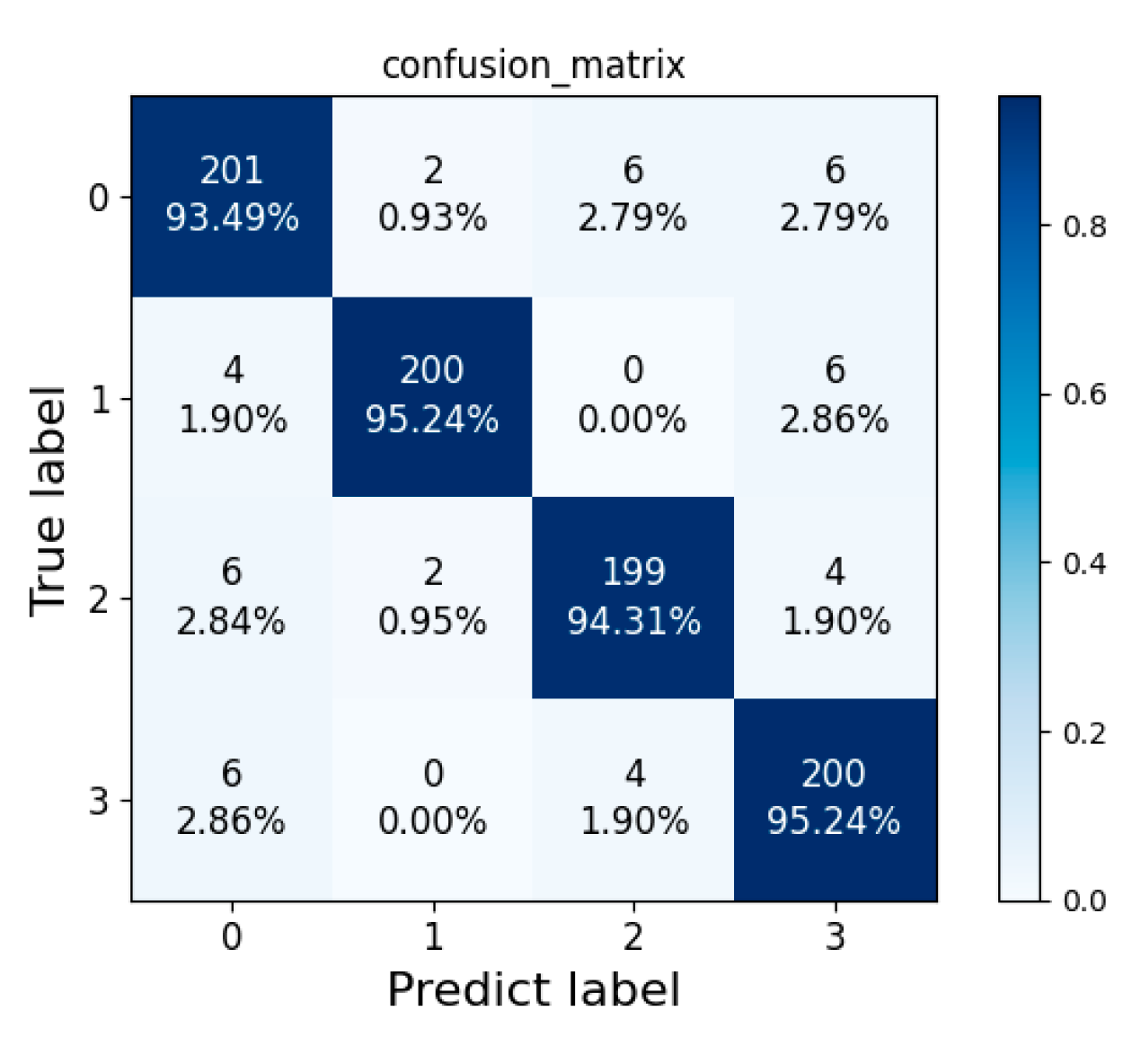
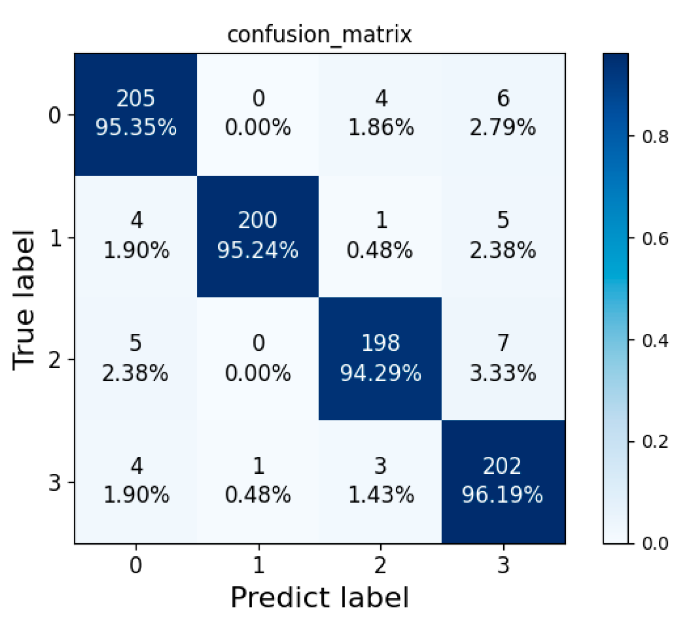
4.3.2. Comparison of Classification Results
- (1)
- Precision:
- (2)
- Recall:
- (3)
- Specificity:where denote true positive, false positive, true negative, and false negative, respectively. The comparative analysis of the classification and identification results of the damage categories of the pipe’s inner wall under different classifiers by the three evaluation indexes above is shown in Table 4.
5. Conclusions
Author Contributions
Funding
Institutional Review Board Statement
Informed Consent Statement
Data Availability Statement
Conflicts of Interest
References
- Qi, P.; Li, T.; Hu, C.; Li, Z.; Bi, Z.; Chen, Y.; Zhou, H.; Su, Z.; Li, X.; Xing, X.; et al. Effects of cast iron pipe corrosion on nitrogenous disinfection by-products formation in drinking water distribution systems via interaction among iron particles, biofilms, and chlorine. Chemosphere 2022, 292, 133364. [Google Scholar] [CrossRef]
- Lee, Y.-H.; Kim, G.-I.; Kim, K.-M.; Ko, S.-J.; Kim, W.-C.; Kim, J.-G. Localized Corrosion Occurrence in Low-Carbon Steel Pipe Caused by Microstructural Inhomogeneity. Materials 2022, 15, 1870. [Google Scholar] [CrossRef] [PubMed]
- De Clercq, D.; Smith, K.; Chou, B.; Gonzalez, A.; Kothapalle, R.; Li, C.; Dong, X.; Liu, S.; Wen, Z. Identification of urban drinking water supply patterns across 627 cities in China based on supervised and unsupervised statistical learning. J. Environ. Manag. 2018, 223, 658–667. [Google Scholar] [CrossRef]
- Dai, L.S.; Wang, T.; Deng, C.Y.; Feng, Q.S.; Wang, D.P. New Method to Identify Field Joint Coating Failures Based on MFL In-Line Inspection Signals. Coatings 2018, 8, 86. [Google Scholar] [CrossRef] [Green Version]
- Miao, X.J.; Li, X.B.; Hu, H.W.; Gao, G.J.; Zhang, S.Z. Effects of the Oxide Coating Thickness on the Small Flaw Sizing Using an Ultrasonic Test Technique. Coatings 2018, 8, 69. [Google Scholar] [CrossRef] [Green Version]
- Rayhana, R.; Jiao, Y.T.; Zaji, A.; Liu, Z. Automated Vision Systems for Condition Assessment of Sewer and Water Pipelines. IEEE Trans. Autom. Sci. Eng. 2021, 18, 1861–1878. [Google Scholar] [CrossRef]
- Medeiros, F.; Ramalho, G.; Bento, M.P.; Medeiros, L. On the evaluation of texture and color features for nondestructive corrosion detection. Eurasip J. Adv. Signal Process. 2010, 817473. [Google Scholar] [CrossRef] [Green Version]
- Hoang, N.D.; Duc, T.V. Image Processing-Based Detection of Pipe Corrosion Using Texture Analysis and Metaheuristic-Optimized Machine Learning Approach. Comput. Intell. Neurosci. 2019, 2019, 8097213. [Google Scholar] [CrossRef] [Green Version]
- Li, S.; Zhou, Z.; Fan, E.; Zheng, W.; Liu, M.; Yang, J. Robust GMM least square twin K-class support vector machine for urban water pipe leak recognition. Expert Syst. Appl. 2022, 195, 116525. [Google Scholar] [CrossRef]
- Atha, D.J.; Jahanshahi, M.R. Evaluation of deep learning approaches based on convolutional neural networks for corrosion detection. Struct. Health Monit. 2018, 17, 1110–1128. [Google Scholar] [CrossRef]
- Papamarkou, T.; Guy, H.; Kroencke, B.; Miller, J.; Robinette, P.; Schultz, D.; Hinkle, J.; Pullum, L.; Schuman, C.; Renshaw, J.; et al. Automated detection of corrosion in used nuclear fuel dry storage canisters using residual neural networks. Nucl. Eng. Technol. 2021, 53, 657–665. [Google Scholar] [CrossRef]
- Kumar, S.S.; Abraham, D.M.; Jahanshahi, M.R.; Iseley, T.; Starr, J. Automated defect classification in sewer closed circuit television inspections using deep convolutional neural networks. Autom. Constr. 2018, 91, 273–283. [Google Scholar] [CrossRef]
- Hassan, S.I.; Dang, L.M.; Mehmood, I.; Im, S.; Choi, C.; Kang, J.; Park, Y.-S.; Moon, H. Underground sewer pipe condition assessment based on convolutional neural networks. Autom. Constr. 2019, 106, 102849. [Google Scholar] [CrossRef]
- Zhang, D.; Gao, W.; Yan, X. Determination of Natural Frequencies of Pipes Using White Noise for Magnetostrictive Longitudinal Guided-Wave Nondestructive Testing. IEEE Trans. Instrum. Meas. 2020, 69, 2678–2685. [Google Scholar] [CrossRef]
- Maeda, Y.; Naruki, K. Gaze Instruction System Used Panoramic Expansion Image of Omnidirectional Camera. In Proceedings of the 2016 Joint 8th International Conference on Soft Computing and Intelligent Systems (SCIS) and 17th International Symposium on Advanced Intelligent Systems (ISIS), Sapporo, Japan, 25–28 August 2016. [Google Scholar]
- Zhang, Q.; Nie, Y.; Zheng, W.S. Dual Illumination Estimation for Robust Exposure Correction; John Wiley & Sons, Ltd.: Hoboken, NJ, USA, 2019. [Google Scholar]
- Tan, L.; Huangfu, T.; Wu, L.; Chen, W. Comparison of RetinaNet, SSD, and YOLO v3 for real-time pill identification. BMC Med. Inform. Decis. Mak. 2021, 21, 324. [Google Scholar] [CrossRef]
- Salkhordeh, M.; Mirtaheri, M.; Soroushian, S. A decision-tree-based algorithm for identifying the extent of structural damage in braced-frame buildings. Struct. Control Health Monit. 2021, 28, e2825. [Google Scholar] [CrossRef]
- Jiang, Z.-P.; Liu, Y.-Y.; Shao, Z.-E.; Huang, K.-W. An Improved VGG16 Model for Pneumonia Image Classification. Appl. Sci. 2021, 11, 11185. [Google Scholar] [CrossRef]
- Xu, H.; Li, C.; Rahaman, M.M.; Yao, Y.; Li, Z.; Zhang, J.; Kulwa, F.; Zhao, X.; Qi, S.; Teng, Y. An Enhanced Framework of Generative Adversarial Networks (EF-GANs) for Environmental Microorganism Image Augmentation with Limited Rotation-Invariant Training Data. IEEE Access 2020, 8, 187455–187469. [Google Scholar] [CrossRef]
- Chen, L.; Liu, R.; Zhou, D.; Yang, X.; Zhang, Q. Fused behavior recognition model based on attention mechanism. Vis. Comput. Ind. Biomed. Art 2020, 3, 7. [Google Scholar] [CrossRef]
- Fei, R.; Yao, Q.; Zhu, Y.; Xu, Q.; Li, A.; Wu, H.; Hu, B. Deep Learning Structure for Cross-Domain Sentiment Classification Based on Improved Cross Entropy and Weight. Sci. Program. 2020, 2020, 3810261. [Google Scholar] [CrossRef]
- Zhang, X.; Hamdulla, A.; Ablimit, M. Multi-lingual Speaker Recognition based on Asymmetric Convolution and Central Loss Function. J. Phys. Conf. Ser. 2021, 2024, 012003. [Google Scholar] [CrossRef]
- Salkhordeh, M.; Alishahiha, F.; Mirtaheri, M.; Soroushian, S. A rapid neural network-based demand estimation for generic buildings considering the effect of soft/weak story. Struct. Infrastruct. Eng. 2022, 1–20. [Google Scholar] [CrossRef]
- Hu, J.; Shen, L.; Albanie, S.; Sun, G.; Wu, E. Squeeze-and-Excitation Networks. IEEE Trans. Pattern Anal. Mach. Intell. 2020, 42, 2011–2023. [Google Scholar] [CrossRef] [Green Version]
- Li, Z.; Li, F.; Zhu, L.; Yue, J. Vegetable Recognition and Classification Based on Improved VGG Deep Learning Network Model. Int. J. Comput. Intell. Syst. 2020, 13, 559–564. [Google Scholar] [CrossRef]
- Hosny, K.M.; Kassem, M.A.; Foaud, M.M. Classification of skin lesions using transfer learning and augmentation with Alex-net. PLoS ONE 2019, 14, e0217293. [Google Scholar] [CrossRef] [Green Version]
- Gao, M.; Qi, D.; Mu, H.; Chen, J. A Transfer Residual Neural Network Based on ResNet-34 for Detection of Wood Knot Defects. Forests 2021, 12, 212. [Google Scholar] [CrossRef]
- Zhang, X.; Chen, X.; Sun, W.; He, X. Vehicle Re-Identification Model Based on Optimized DenseNet121 with Joint Loss. Comput. Mater. Contin. 2021, 67, 3933–3948. [Google Scholar] [CrossRef]
- Jeong, E.; Oh, J.-Y.; Young, L.J.; Hoon-Hee, P. Application of Deep Learning-Based Nuclear Medicine Lung Study Classification Model. J. Radiol. Sci. Technol. 2022, 45, 41–47. [Google Scholar] [CrossRef]


| Sample | Before Data Enhancement | After Data Enhancement |
|---|---|---|
| Pitting corrosion | 783 | 1730 |
| Areal corrosion | 788 | 1739 |
| Slight corrosion | 790 | 1742 |
| Normal pipeline | 724 | 1588 |
| Hyper-Parameter | The Optimal Value |
|---|---|
| batch_size | 32 |
| dropout | 0.5 |
| learning rate | 0.001 |
| regularization factor | 0.5 |
| epoch | 200 |
| weight decay | 0.0005 |
| Corrosion Category | Alex | VGG | Lian-VGG | SE-VGG | ResNet50 | DenseNet121 | Model in This Paper |
|---|---|---|---|---|---|---|---|
| Normal pipeline | 195 | 199 | 199 | 201 | 202 | 200 | 205 |
| Slight corrosion | 189 | 193 | 196 | 200 | 195 | 195 | 200 |
| Pitting corrosion | 190 | 195 | 194 | 199 | 193 | 190 | 198 |
| Areal corrosion | 185 | 192 | 197 | 200 | 199 | 196 | 202 |
| Total number of correct | 759 | 779 | 786 | 800 | 789 | 781 | 805 |
| Classification accuracy | 89.822% | 92.189% | 93.018% | 94.674% | 93.372% | 92.426% | 95.266% |
| Corrosion Category | Classification Models | Precision | Recall | Specificity |
|---|---|---|---|---|
| Normal pipeline | Alex | 88.636% | 90.700% | 96.031% |
| VGG | 90.867% | 92.561% | 96.825% | |
| Lian-VGG | 92.990% | 92.561% | 97.612% | |
| SE-VGG | 92.627% | 93.492% | 97.464% | |
| ResNet50 | 91.402% | 93.953% | 96.984% | |
| DenseNet121 | 91.743% | 93.023% | 97.142% | |
| Algorithms in this paper | 94.037% | 95.354% | 97.936% | |
| Slight corrosion | Alex | 90.865% | 90.001% | 97.007% |
| VGG | 95.544% | 91.903% | 98.582% | |
| Lian-VGG | 96.078% | 93.334% | 98.740% | |
| SE-VGG | 98.035% | 95.242% | 99.371% | |
| ResNet50 | 97.014% | 92.857% | 99.063% | |
| DenseNet121 | 94.660% | 92.847% | 98.307% | |
| Algorithms in this paper | 99.502% | 95.46% | 99.842% | |
| Pitting corrosion | Alex | 88.785% | 92.381% | 96.220% |
| VGG | 90.278% | 92.863% | 96.692% | |
| Lian-VGG | 90.654% | 92.389% | 96.850% | |
| SE-VGG | 95.215% | 94.318% | 98.425% | |
| ResNet50 | 93.689% | 91.905% | 98.006% | |
| DenseNet121 | 93.137% | 90.476% | 97.862% | |
| Algorithms in this paper | 96.116% | 94.295% | 98.740% | |
| Areal corrosion | Alex | 91.133% | 88.108% | 97.165% |
| VGG | 92.307% | 91.436% | 97.480% | |
| Lian-VGG | 92.488% | 93.813% | 97.480% | |
| SE-VGG | 92.592% | 95.246% | 97.637% | |
| ResNet50 | 91.705% | 94.761% | 97.166% | |
| DenseNet121 | 90.323% | 93.334% | 96.692% | |
| Algorithms in this paper | 91.8188% | 96.192% | 97.165% |
Publisher’s Note: MDPI stays neutral with regard to jurisdictional claims in published maps and institutional affiliations. |
© 2022 by the authors. Licensee MDPI, Basel, Switzerland. This article is an open access article distributed under the terms and conditions of the Creative Commons Attribution (CC BY) license (https://creativecommons.org/licenses/by/4.0/).
Share and Cite
Zhao, Q.; Li, L.; Zhang, L. Identification of Corrosion on the Inner Walls of Water Pipes Using a VGG Model Incorporating Attentional Mechanisms. Appl. Sci. 2022, 12, 12731. https://doi.org/10.3390/app122412731
Zhao Q, Li L, Zhang L. Identification of Corrosion on the Inner Walls of Water Pipes Using a VGG Model Incorporating Attentional Mechanisms. Applied Sciences. 2022; 12(24):12731. https://doi.org/10.3390/app122412731
Chicago/Turabian StyleZhao, Qian, Lu Li, and Lihua Zhang. 2022. "Identification of Corrosion on the Inner Walls of Water Pipes Using a VGG Model Incorporating Attentional Mechanisms" Applied Sciences 12, no. 24: 12731. https://doi.org/10.3390/app122412731