Article

Back Analysis of Geotechnical Engineering Based on Data-Driven Model and Grey Wolf Optimization

1
School of Fine Art, Shandong University of Technology, Zibo 255000, China
2
School of Civil and Architectural Engineering, Shandong University of Technology, Zibo 255000, China
*
Author to whom correspondence should be addressed.
Appl. Sci. 2022, 12(24), 12595; https://doi.org/10.3390/app122412595
Submission received: 21 September 2022 / Revised: 25 November 2022 / Accepted: 27 November 2022 / Published: 8 December 2022
(This article belongs to the Special Issue The Application of Machine Learning in Geotechnical Engineering)

Abstract

:
Geomaterial mechanical parameters are critical to implementing construction design and evaluating stability through feedback analysis in geotechnical engineering. The back analysis is widely utilized to identify and calibrate the geomaterial mechanical properties in geotechnical engineering. This study developed a novel back-analysis framework by combining a reduced-order model (ROM), grey wolf optimization (GWO), and numerical technology. The ROM was adopted to evaluate the response of the geotechnical structure based on a numerical model. GWO was used to search and identify the geomaterials properties based on the ROM. The developed back analysis framework was applied to a circular tunnel and a practical tunnel for determining the mechanical property of the surrounding rock mass. The results showed that the ROM could be an excellent surrogated model and replaced it with the numerical model. The obtained geomaterial properties were in excellent agreement with the actual properties. The deformation behavior captured by the developed framework was consistent with the theoretical solution in a circular rock tunnel. The developed framework provides a practical, accurate, and convenient approach for calibrating the geomaterial properties based on field monitoring data in practical geotechnical engineering applications.

1. Introduction

The geomaterial property is critical to guiding construction and assuring safety during the feedback analysis and dynamic design for geotechnical engineering [1,2,3]. The back analysis based on field monitoring data has been widely used in geotechnical engineering. The back analysis aims to obtain the geomaterial properties by minimizing the objective function, which represents the response difference of geotechnical structure between the monitored field and the predicted by the physical model, based on the optimization technology. The core of the back analysis technique is the optimization technique and physical model. Generally, the numerical method is widely used to calculate the structure response field in practical geotechnical engineering [4,5]. However, a numerical method is time-consuming due to the repetitive computing in back analysis, especially for the practical large-scale geotechnical structure. Meanwhile, optimal techniques often have problems in back analysis, such as high dimensionality, complexity, and local minima. In order to solve the above two problems, various surrogate models and optimal technology have been proposed in the back analysis [2,3,6]. In this study, the reduced order model (ROM) and the grey wolf algorithm (GWO) were combined to improve the practicability of back analysis.
Last century, displacement back analysis was proposed by Sakurai and Takeuchi to identify the rock mechanical parameters based on the monitoring information of the tunnel [7]. However, the numerical method is time-consuming and limits the engineering application of back analysis. In order to overcome the limitations of the numerical method, various machine learning-based surrogate models were a focus of attention to approximate the response of the geotechnical structure in the past decades [8,9,10,11]. The neural network method was utilized to construct the intelligent displacement back analysis model for identifying the mechanical property of the surrounding rock mass [12,13,14,15]. The support vector machine and the relevance vector machine were selected to build a displacement back analysis model to recognize the geomaterials parameters [16,17,18]. Machine learning provides an excellent tool for predicting the structural response and is selected as the surrogate model in the geotechnical back analysis. However, some limits of artificial intelligence, such as overfitting, trapping local minimum, etc., hinder the practical application in back analysis for geotechnical engineering. Meanwhile, the traditional surrogate model does not reflect the physical mechanism of geological engineering and only obtains information about the discrete response at some monitoring points. Therefore, obtaining the total response fields using this classical approach is challenging due to the learning efficiency. The ROM was developed that contains some knowledge about the engineering structure under consideration and can overcome the limits of machine learning and the traditional surrogate model. So, this study adopted the ROM to establish the surrogate model for back analysis.
In order to acquire the appropriate geomaterial property, various intelligent optimization methods, such as genetic algorithm [16,19,20], artificial bee colony [18], particle swarm optimization [21,22], etc., have been widely utilized to seek the geomechanical property in the back analysis. Due to the complexity of geomaterials, trapping the local minimum solution is the main drawback of the back analysis method, which hinders its application in practical engineering. Grey wolf optimization (GWO) is an efficient metaheuristic method developed recently [23]. The GWO algorithm is suitable for solving nonlinear and complex problems due to its simple concept, small number of adjustable parameters, fast convergence, and strong global optimization capacity. It only considers the function evaluation and does not need the derivative information, which is suitable for black box global optimization problems. So, GWO was selected as an optimal technology for the back analysis in this study.
This study proposed a novel back analysis approach by combining numerical models, ROM, and GWO to identify the geomaterial mechanical property in geotechnical engineering. ROM was utilized to construct a surrogate model to approximate and capture the response of the geotechnical structure for replacing the numerical model in the back analysis. The GWO algorithm was regarded as an optimal technology for seeking the unknown geomaterial property based on the idea of the back analysis. The developed framework was applied to a circular tunnel and an actual tunnel project. The remainder of this study is stated as follows. First, ROM and GWO algorithms are briefly introduced in Section 2 and Section 3, respectively. Section 4 introduces the main ideas and procedures of the developed back analysis in detail. In Section 5, a circular tunnel and an actual tunnel, i.e., the experimental tunnel in the Goupitan Water conservancy project, China, are used to verify and investigate the developed back analysis framework. Finally, some conclusions are drawn in Section 6.

2. Reduced-Order Model

2.1. Constructing the ROM Model

The ROM was used to predict the system response using a low-order model based on numerical methods and the proper orthogonal decomposition in engineering. For any xi, i = 1, 2, …, I, and θj, j = 1, 2, …, J, the proper orthogonal decomposition was utilized to obtain the following equation [24].
u ˜ h ( x i , θ j ) = k = 1 K β k ( θ j ) φ k ( x i ) + g ˜ ( x i , θ j )
where u ˜ h denots the solution of field variables for geotechnical structure, θj and xi denote the parameter and design variables of a geotechnical model, φ and β note the unknown coefficient of ROM, and g ˜ ( x , θ ) is an extended boundary condition in the entire domain.
g ˜ ( x , θ ) = { g ( x , θ )   o n   0   e l s e w h e r e
Equation (1) can be rewritten as follows:
u ˜ h = φ β + g ˜
By utilizing the Latin hypercube sampling (LHS), the set of design variables θ j ,   j = 1 , 2 , , J . was constructed for determining the unknown coefficient φ . Then, the corresponding discrete solutions (snapshots) of the numerical model w j = u h ( θ j ) g ˜ ( θ j ) ,   j = 1 , 2 , , J , were acquired based on numerical techniques such as finite element, discrete element, boundary element, etc. The spatial Gram matrix by Mx can be obtained as follows:
M i j x = ( w i · w j ) ,   i , j = 1 , 2 , , J
where ( w i · w j ) notes the inner product between wi and wj.
The descending order of the positive eigenvalues of Mx is listed in the following form.
λ 1 λ 2 λ J 0
The first K eigenfunctions φ k ( x ) ,   k = 1 , 2 , K corresponds to the first K eigenvalues, providing the orthogonal principal direction of snapshots. If r k = ( r j k ) j = i , i , J denotes the kth eigenvector of Mx, then its dual kth eigenfunctions φ k ( x ) can be determined according to the following form.
φ k ( x ) = j = 1 K r j k w j ( x )
where K notes the basis size of the proper orthogonal decomposition and can be solved in the following inequation.
i = 1 K λ i i = 1 J λ i > k
where k is the user-specified tolerance and equals 0.9999 in this study.
The following penalized minimization problem can solve the unknown coefficient β.
min β j R K u h , j φ β j g ˜ j 2 + μ β j 2
β j can be solved by the following normal equation.
( φ T φ + μ I K ) β j = φ T ( u h , j g ˜ j ) ,   j = 1 , 2 , , J
where μ notes a small regularization parameter.

2.2. Predicting the Field Variables

In order to determine the field variables for unknown variables θ and x, the radial basis function (RBF) was adopted to expand the coefficient β k ( θ ) in the following form.
β k ( θ ) = j = 1 J α j k ψ ( | θ θ j | σ )
For any θ j ,   j = 1 , 2 , , J , Equation (10) can be presented as follows.
j = 1 J α j k ψ ( | θ j θ j | σ ) = β k j
where β k j are determined by Equation (9). The above equations can be rewritten in the compacted form:
A α k = β k
The following equation can solve the unknown coefficient α k .
( A T A + μ I J ) α k = A T β k ,   k = 1 , 2 , , K

2.3. Procedure of the ROM Model

This study developed a ROM by combining the numerical method (including finite element, discrete element and boundary element, etc.) and the proper orthogonal decomposition. Using the LHS, the set of design variables was constructed for the snapshot. Then the numerical method was adopted to calculate the corresponding solution of design variable in the above set. Based on the obtained snapshots, the proper orthogonal decomposition basis vector and its coefficient were acquired using the proper orthogonal decomposition algorithm for geotechnical engineering. In order to acquire the unknown field of the new design variable, RBF functions were adopted to expand the coefficient of the proper orthogonal decomposition basis and then to determine the coefficients of the orthogonal decomposition ROM. The unknown field variables corresponding to the new design were determined using the ROM. Figure 1 shows the main flowchart and procedure of the ROM. In what follows, the procedure of the ROM model is presented in detail.
  • Step 1: Collect the data of the geotechnical engineering, including project property, geo-stress, boundary conditions, etc.;
  • Step 2: Establish the numerical model (FEM) based on the above engineering information;
  • Step 3: Construct the design variables set θ for the numerical model using LHS;
  • Step 4: Calculate the field variables wi (displacement or stress field) at space domain X using a numerical method for each design variable. Collect all the field variables and acquire the snapshots;
  • Step 5: Build the spatial Gram matrix Mx based on the above snapshots;
  • Step 6: Solve the eigenvalues λ and eigenvectors r based on the spatial Gram matrix;
  • Step 7: Determine the rank number K of Mx and the first K eigenfunction vector φ;
  • Step 8: Determine the undetermined coefficient β based on eigenfunction vector φ and snapshots;
  • Step 9: To a new design variable θ, construct element ɸ based on the design variables θ generated by LHS using the RBF function;
  • Step 10: Determine the interpolation matrix A of elements ɸ;
  • Step 11: Determine the vector of element α using the penalized linear systems;
  • Step 12: Solve the coefficients β(θ) based on the RBF function;
  • Step 13: Calculate the unknown field variables u ˜ h ( θ ) based on coefficients β(θ) and eigenfunction vector φ using the ROM.

3. Grey Wolf Optimization (GWO)

Grey Wolf Optimization (GWO) is a heuristic optimization strategy inspired by the social hierarchy and hunting techniques of grey wolves. GWO mimics the leadership hierarchy and hunting technology of grey wolves. The hierarchy of the grey wolves is divided into four levels (alpha (α), beta (β), delta (δ), and omega (ω)), which present the optimal solution, the suboptimal solution, the third optimal solution, and the remaining candidate solutions, respectively [23]. There are three main stages of grey Wolf hunting, namely searching, encircling, and attacking prey. The GWO is the mathematical model of the hunting strategy and social hierarchy of grey wolf. A grey wolf can determine the prey by randomly changing its position based on the GWO algorithm. The hunting process is guided by α, β, δ, and ω according to the above three kinds of wolves in GWO.
In the encircling phase, the encircling behavior of wolves can be expressed in the following mathematical model:
D = | D X p ( t ) X ( t ) |
X ( t + 1 ) = X p ( t ) A D
where t denotes the step of the iteration, D denotes the searching vector, X and X p are the vector and denote the position of a grey wolf and the prey, respectively. A and C denote the coefficient vectors and can be determined according to the following form:
A = 2 a r 1 a
C = 2 r 2
where r 1 and r 2 denote the vector and selected randomly in the range of zero to unity, the component a decreases linearly from 2 to 0 with the iterations.
In the hunting phase, the locations of other search agents (including omega) were updated according to alpha, beta, and delta knowledge based on the following equations.
D α = | C 1 X α X |
D β = | C 2 X β X |
D δ = | C 3 X δ X |
X 1 = X α A 1 D α
X 2 = X β A 2 D β
X 3 = X δ A 3 D δ
X ( t + 1 ) = X 1 + X 2 + X 3 3
where the subscripts α, β, and δ represent the alpha wolf, beta wolf, and delta wolf, respectively.
In the attacking prey phase, the final attack is determined by decreasing the a from 2 to 0 with the iterations A selected randomly in the range [ 2 a , 2 a ]. A will decrease with the reduction to the a and force the wolfs to approach the prey while | A | is less than 1.
In search of prey, grey wolves follow the leader, dispersing from one another in search of prey and gathering to attack. The number of wolves Nw and the generation NG are the two essential parameters of GWO. Each generation represents the decision movement of a wolf. The number of wolves represents the function computational times in each generation. Figure 2 shows the flowchart of GWO and the main procedure. A detailed introduction of the GWO can be found in the literature [23].

4. ROM-Based Back Analysis Using GWO

Back analysis technology has been commonly utilized to identify the geomaterial property in geotechnical engineering. The numerical method and the optimal technology are the two critical elements of back analysis. This study developed a ROM-based back analysis combining numerical methods, ROM, and GWO. The ROM model was utilized to predict the nonlinear response of the geotechnical structure based on the numerical method. GWO was selected as an optimal technology to seek the geomaterial properties.

4.1. Back Analysis

In the 1970s, back analysis was proposed to identify the rock mass properties in rock engineering [25]. The back analysis provides a simple but effective way to identify the geomaterial properties based on the field data and numerical analysis. It also provides a helpful tool for guiding the dynamic design, reinforcement of surrounding rock mass, and safe construction of geotechnical engineering. Figure 3 shows the main parts of the back analysis and its basic idea. Field measurements provide basic information for back analysis. The physical model is the heart of the back analysis. Due to the complex geological conditions, it is not easy to determine the closed-form solution of geotechnical engineering. Meanwhile, optimal technology is essential to back analysis due to multi-extremum and multi-constrained optimization problems. This study adopted the ROM model to capture the physical model. GWO was selected as the optimal technology due to its excellent global optimizing capability.

4.2. ROM-Based Surrogate Model

The physical model characterizes the nonlinear implicit function mapping between geomaterial properties and their response during construction. In this study, a ROM-based physical model was established to capture the nonlinear mapping function between the geomaterial properties (Deformation modulus, Poisson’s ratio, strength property, and in-situ stress) and corresponding structural response (displacement, stress, strain, etc.). The following equations define the physical model ROM(X).
R O M ( X ) : R N R Q ,
Y = ROM (X),
where X = (x1, x2, …, xN) is a vector and xi (i = 1, 2, …, N) is the ith geomaterial properties and Y = (y1, y2, …, yN) is a Q dimension vector and denotes the response induced by construction.
Some known training samples are necessary for establishing the surrogate model ROM(X) of the physical model in the back analysis. It is necessary to obtain the training samples for ROM based on a numerical method and the design of experiment.

4.3. Objection Function

This study constructed the objective function based on the geotechnical structure response difference between the field value and ROM prediction. The objection function forced the optimal technology to seek the optimal variable. The following root means square defines the objective function:
f i t n e s s = i = 1 n ( y p i y i ) 2 / n
where n denotes the number of monitoring points, yi and ypi denote the predicted by ROM and monitoring response of the geotechnical structure in ith measurement point.

4.4. Procedure of the Developed Framework

This study developed a novel back-analysis framework combining ROM, GWO, and numerical technology. The ROM was adopted to capture the nonlinear mapping between the geomaterial properties and the corresponding response during excavation in combination with the ROM and numerical model. The experimental design was adopted to construct the combination of the unknown properties, and then the numerical method was utilized to calculate the structural response at each combination. The snapshots consist of a combination of the unknown parameters and the corresponding response. ROM was built based on the above snapshots. GWO is an optimal approach to seeking geomaterial properties based on the ROM. The detailed procedures of the proposed method are listed as follows (as seen in Figure 4):
  • Step 1: Collect the engineering data, such as the unknown (need to determine by back analysis) and known geomaterial mechanical and physical properties, boundary conditions, and the range of unknown geomaterial properties;
  • Step 2: Generate the combination of the unknown properties based on experimental design and calculate the structural response at each training sample. The snapshots consist of the combination of the unknown parameters and the corresponding response;
  • Step 3: Based on the determined snapshots, generate the ROM to capture the nonlinear function mapping between the geomaterial properties and the corresponding structural response in geotechnical engineering;
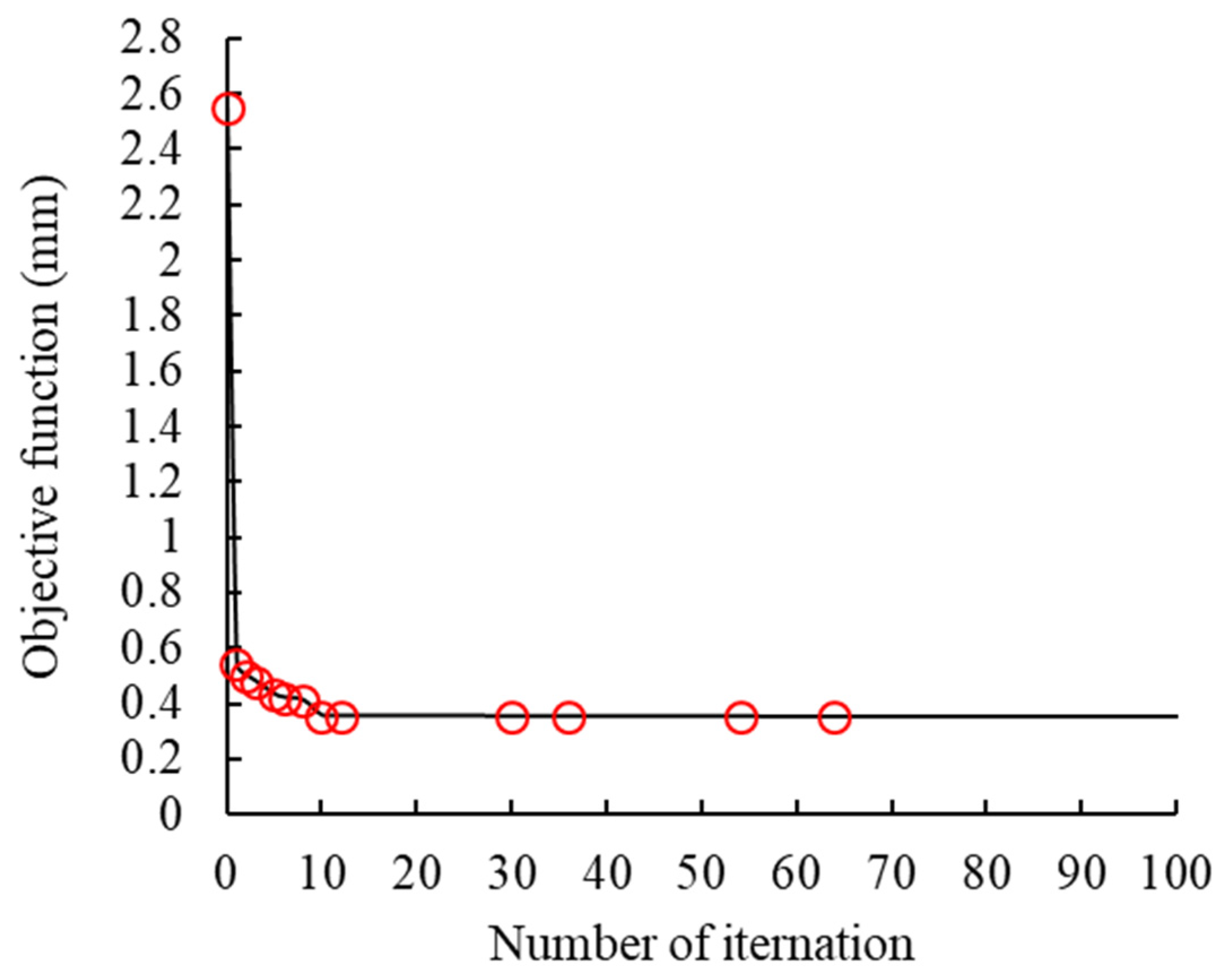
  • Step 4: Establish the objective function and call the GWO to seek the geomaterial properties based on the monitored data during the construction.

5. Numerical Example and Application

5.1. Numerical Example

A circular tunnel is excavated in a continuous, homogeneous, and isotropic rock mass. The hydrostatic far-field stress p0 and uniform support pressure pi are shown in Figure 5. When support pressure pi is not enough to meet critical pressure pcr, a plastic zone will exist. The values of pcr could be computed as follows:
p c r = 2 p 0 σ c k + 1
where σc notes the uniaxial compression strength. It could be obtained using the following equation.
σ c = c ( k 1 ) tan φ
where φ and c denote the cohesion and the friction angle, respectively. k could be determined as follows:
k = 1 + sin φ 1 sin φ
According to the Mohr–Coulomb criterion, Duncan (1993) analyzed and inferred the inward displacement of tunnel wall uip and the plastic zone radius rp [26].
r p r 0 = [ 2 ( p 0 + s ) ( k + 1 ) ( p i + s ) ] 1 k 1
u i p r 0 = [ ( 1 + μ ) E ] [ 2 ( 1 μ ) ( p 0 p c r ) ( r p r 0 ) 2 2 ( 1 2 μ ) ( p 0 p i ) ]
where E notes the elastic modulus and μ notes Poisson’s ratio. The values are computed as follows:
s = σ c k 1
In this study, back analysis was utilized to identify the far-field stress p0, cohesion c, and friction angle φ based on the deformation of the surrounding rock mass in the tunnel. Five horizontal direction monitoring points were placed to record the deformation of surrounding rock mass in the circular tunnel. The distance between the center of the tunnel and the five monitored points are 1.0 m, 1.2 m, 1.6 m, 1.8 m, and 2.0 m, respectively. The displacements of monitored points could be calculated using the above formula (Equation (32)). The tunnel radius is 1.0 m. The value of far-field stress p0, cohesion c, and friction angle φ are 32 MPa, 6.8 GPa, 3.2 MPa, and 32°, respectively. The displacements of 5 monitored points were calculated by the analytical solution and adopted as field measurement to back-calculate the unknown parameters of the surrounding rock mass using the proposed method. The snapshots were constructed and generated based on the experimental design and a numerical method.
Once the snapshots are obtained, the surrogate model could be established according to the ROM algorithm. Figure 6 shows the calculated displacement comparison between the ROM and the analytical solution (Equation (32)). The predicted displacement using the ROM surrogate model is in good agreement with the analytical solution. It shows that the ROM captured well the nonlinear function mapping between unknown properties and the tunnel deformation. The ROM-based surrogate model provides a feasible way to replace the analytical solution in back analysis.
ROM-based back analysis was utilized to identify the unknown properties of the surrounding rock mass using the above ROM surrogate model and to predict displacement in the tunnel. The far-field stress p0, cohesion c, and friction angle φ are 32.01 MPa, 6.73 GPa, 3.40 MPa, and 31.03°, respectively (Table 1). The relative error is −0.03%, 1.02%, −6.25% and 3.03%, respectively. The maximum relative error is less than 7%. It shows that the identified parameters agree with the actual parameters using the proposed back analysis framework. The displacements comparison between the predicted by back analysis, ROM surrogate model, and calculated by the analytical by actual parameters are shown in Figure 7. Figure 8 shows the stress and displacement of the surrounding rock mass in the tunnel calculated based on the different methods. The results show that the proposed framework can be utilized to identify the mechanical property of the surrounding rock mass in the tunnel.
Figure 9 shows the convergence of the unknown mechanical property of the surrounding rock mass using the developed back analysis method. The convergence property of the developed back analysis is shown in Figure 10. The unknown property can converge to the final value quickly. The developed method has excellent convergence and global optimization performance.

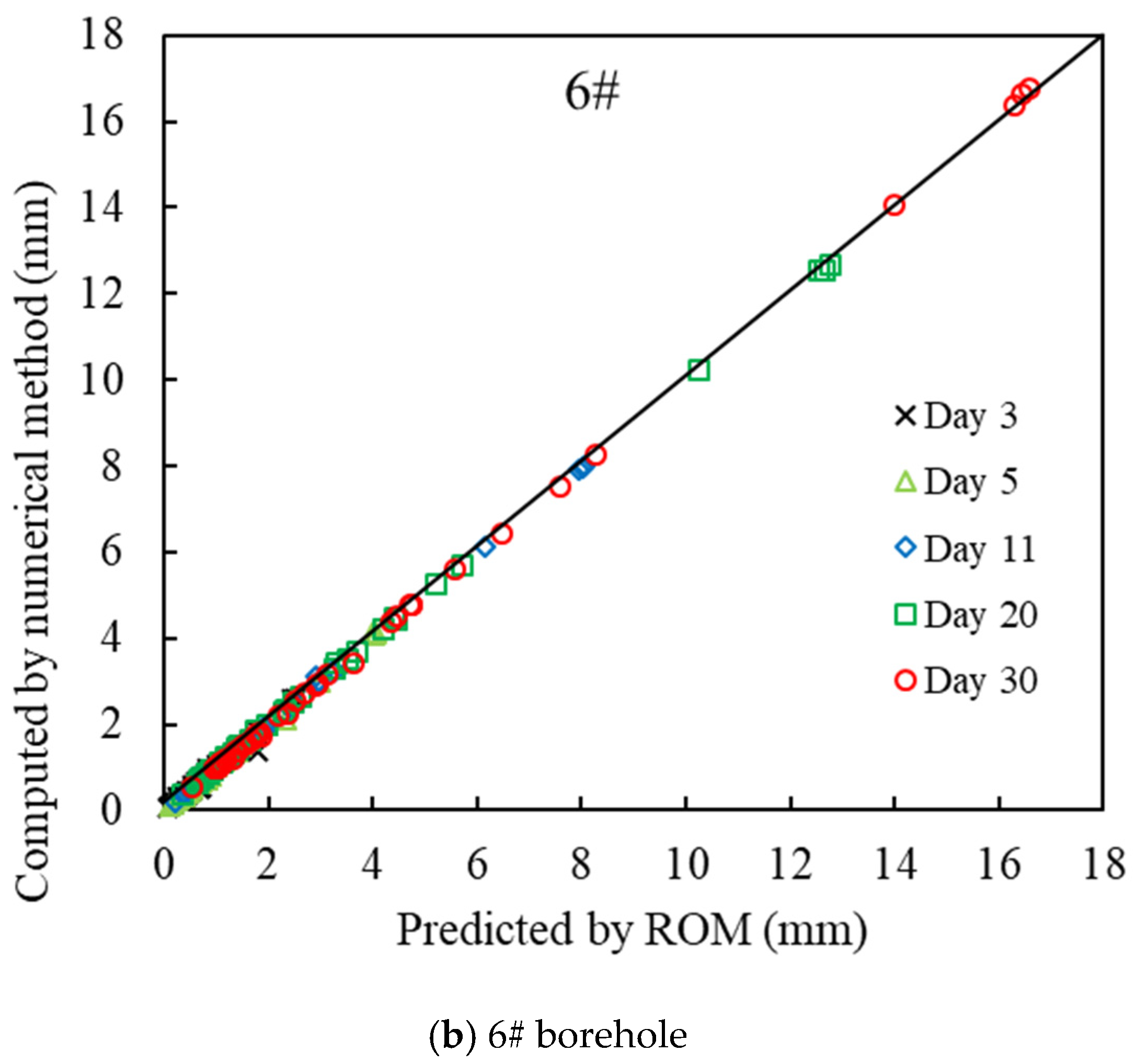
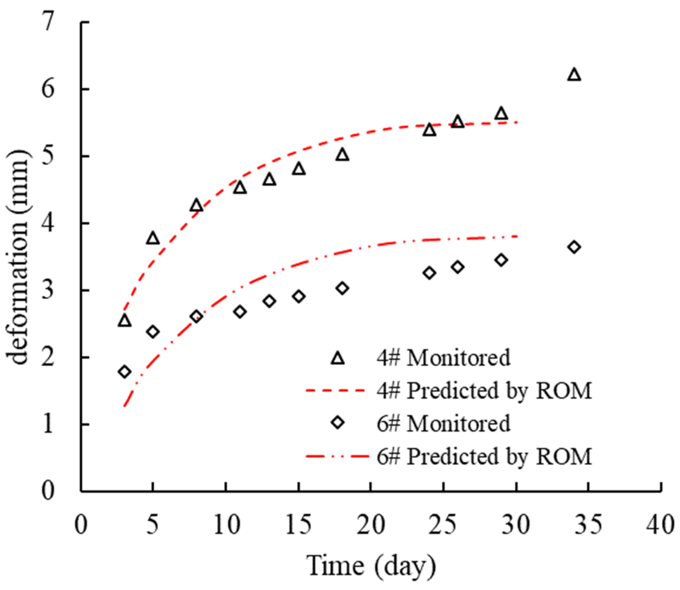
5.2. Application: Goupitan Experimental Tunnel

Goupitan Hydropower Station is a landmark west-to-east transmission project located on the Wujiang River in Guizhou Province, China [27]. According to the preliminary design of the underground powerhouse, the right bank tailwater tunnel and the construction diversion tunnel pass through the soft clay rock mass. An experiment tunnel with a buried depth of 70 m was excavated to understand the rheological characteristics of clay rock. The tunnel size was 2 m in width and 2 m in height, respectively. Some monitoring points are set up to obtain the deformation of surrounding rock during tunnel excavation. Rock stratum S 2 h 1 2 and S 2 h 1 1 are located approximately 3 m below and 30 m above the tunnel, respectively (Figure 11). The 4# and 6# borehole of 7 m depth is set at the position of 11.6 m in the tunnel, where the 4# borehole is horizontal, the 5# borehole is 45° inclined, and the 6# borehole is vertical. Five monitoring points numbered 1–5 were arranged at a depth of 0, 1, 2, 4, and 6 m (Figure 11). Table 2 lists the deformation of the 3-day, 5-day, and 11-day at each monitoring point.
The developed back analysis framework was utilized to identify the rheological properties of the rock mass based on the 3rd, 5th, and 11th day monitored displacements at 4# and 6# boreholes. For the developed back analysis, a physical model is critical to identify the rheological mechanical properties of the rock mass. In this study, the rheological properties of the rock mass include the shear modulus G1 and viscosity η1 for the Kelvin model, the shear modulus G2 and viscosity η2 for the Maxwell model. In geotechnical engineering, it is not easy to determine an analytical solution for use. Although the numerical method is commonly used to understand the rheological mechanism and deformations behavior of the rock mass, it is time-consuming in practical and large-scale geotechnical engineering.
In this study, a ROM surrogate model, which replaced the numerical method, was used to improve the efficiency of back analysis. A uniform design was utilized to construct a group of 42 samples, and Fast Lagrangian Analysis of Continua (FLAC) software was utilized to solve the displacement of the tunnel wall in the rock mass. Rock masses S 2 h 1 1 and S 2 h 1 2 were regarded as Burger‘s material [28,29], and their rheological mechanical properties were identified by the developed method. Table 3 lists the range of unknown rheological mechanical parameters based on laboratory tests and a field survey. Figure 12 indicates the predicted displacement comparison by the ROM and the numerical model along 4# and 6# boreholes, respectively. The calculated deformations by the ROM were found very close to the deformation computed by the numerical solution. It proves that the ROM surrogate model characterized well the nonlinear mapping relationship between unknown rheological properties and deformation of the tunnel wall in the rock mass. Hence, it could replace the numerical method in the back analysis.
According to the back analysis theory and the proposed method, the rheological parameters of S 2 h 1 1 and S 2 h 1 2 are determined based on the displacement of the surrounding rock mass on the 3rd, 5th and 11th days of the 4# and 6# boreholes (Table 4). The developed method identified the rheological mechanical properties in a reasonable way. Compared with other methods, the rheological mechanical properties obtained by the proposed framework are closer to the actual properties of rock mass, and the rheological properties could be determined dynamically by rationally using the on-site displacement data monitored during construction. The developed back analysis framework costs approximately 73.65 s in PC with Intel(R) Xeon(R) Gold 5218 CPU @ 2.30 GHz &2.29 GHz to obtain the rheological properties. However, it takes approximately 2 min for a single tunnel stability analysis using the numerical simulation method. It is obvious that the ROM-based surrogate model could dramatically improve the efficiency of back analysis.
It is critical to identify and understand the deformation and failure mechanism of the surrounding rock mass. The developed back analysis identifies the rheological properties based on the displacements monitored. The deformation of the rock mass was investigated based on the rheological properties identified by the developed back analysis framework using the ROM and GWO. The ROM then predicted the displacements of the monitored borehole. Their comparisons are shown in Figure 13 in which it is evident that the displacement determined by the ROM is in good agreement with the monitored displacement during the excavation. It also shows that the identified rheological properties well characterized the rheological behavior of the rock mass during the tunnel construction. This confirms that the developed method can be used for determining rheological properties and evaluating the time-dependent behavior of the rock mass. The rheological properties obtained by the developed method can be used for stability analysis, design, and safety construction during excavation in rock engineering. In addition, the predicted deformation by ROM diverges from the monitoring data on the 34th day due to the complexity of the construction site, which brings errors and uncertainty to the monitoring data. With the increasing monitoring data, the rheological properties of the surrounding rock mass will be updated dynamically to capture the trend.
The relationship between the rheological property (clay-green clay rock) and the number of iterations is shown in Figure 14 for the GWO. The variation process objective function is plotted in Figure 15. The results are similar to the above numerical example. GWO could seek the appropriate mechanical property of the rock mass quickly. It proved again that the GWO is an excellent optimal technology and has a good performance of global optimization.

6. Conclusions

This study developed a novel back analysis framework to identify the geomaterial property by combining a numerical model, ROM, and GWO. The ROM was utilized to establish the surrogate model for capturing deformation during excavation in geotechnical engineering. The numerical method was adopted to construct snapshots for the ROM based on the design of the experiment. The geomaterial properties were identified based on the monitored displacement data by the developed framework. Meanwhile, GWO was selected as an optimal technology for back analysis due to its global optimization performance. The developed back analysis framework was illustrated successfully by a numerical example and Goupitan experimental tunnel. The geomaterial properties identified by this study were compared with the ROM prediction. The predicted displacement of the surrounding rock mass was also close to the actual monitored displacement. The results showed that the developed back analysis framework provides a convenient, practical, and accurate way to understand the geomaterial properties based on the monitored response during construction.
(1)
The ROM model was utilized to construct a low-order surrogate model for capturing the response-induced excavation in geotechnical engineering and replacing the numerical model in the back analysis. It is critical to practical engineering due to the difficulties in obtaining the analytical solution for geotechnical engineering;
(2)
Back analysis is a scientific and practical tool widely used in geotechnical engineering. The numerical model and optimal technology are the two critical components of back analysis. The developed back analysis framework takes full advantage of the merits of ROM and GWO and provides a feasible way for determining the property of the surrounding rock mass in geotechnical engineering;
(3)
ROM is an excellent physics-based data-driven surrogate model that can capture the mechanism of surrounding rock mass. GWO is an efficient metaheuristic method developed recently and is suitable for solving the black-box problem. However, ROM depends on the numerical fidelity model, and the parameters of the GWO algorithm influence the optimal performance. In a future study, the authors will further improve the developed framework by absorbing and combining the advantages and merits of various methods.

Author Contributions

Conceptualization, L.Z. and H.Z.; methodology, L.Z. and H.Z.; software, L.Z. and H.Z.; validation, X.L. and X.Z.; formal analysis, L.Z. and H.Z.; investigation, L.Z. and H.Z.; data curation, L.Z. and H.Z.; writing—original draft preparation, L.Z. and H.Z.; writing—review and editing, X.L. and X.Z.; visualization, H.Z. All authors have read and agreed to the published version of the manuscript.

Funding

This study is sponsored in part by the Shandong Provincial Natural Science Foundation, China under grant ZR2022ME198, to which the authors are very grateful.

Institutional Review Board Statement

Not applicable.

Informed Consent Statement

Not applicable.

Data Availability Statement

The data presented in this study are available on request from the corresponding author.

Conflicts of Interest

The authors declare no conflict of interest.

References

  1. Zhao, Z. A practical and efficient reliability-based design optimization method for rock tunnel support. Tunn. Undergr. Space Technol. 2022, 127, 104587. [Google Scholar] [CrossRef]
  2. Zhao, H.; Chen, B.; Li, S.; Li, Z.; Zhu, C. Updating models and the uncertainty of mechanical parameters for rock tunnels using Bayesian inference. Geosci. Front. 2021, 12, 101198. [Google Scholar] [CrossRef]
  3. Zhao, H.; Chen, B.; Li, S. Determination of geomaterial mechanical parameters based on back analysis and reduced-order model. Comput. Geotech. 2021, 132, 104013. [Google Scholar] [CrossRef]
  4. Jing, L.; Hudson, J.A. Numerical methods in rock mechanics. Int. J. Rock Mech. Min. Sci. 2002, 39, 409–427. [Google Scholar] [CrossRef]
  5. Choi, Y.-H.; Lee, S.S. Reliability and efficiency of metamodel for numerical back analysis of tunnel excavation. Appl. Sci. 2022, 12, 6851. [Google Scholar] [CrossRef]
  6. Zhao, H.; Chen, B. Inverse analysis for rock mechanics based on a high dimensional model representation. Inverse Probl. Sci. Eng. 2021, 29, 1565–1585. [Google Scholar] [CrossRef]
  7. Gao, W. A comprehensive review on identification of the geomaterial constitutive model using the computational intelligence method. Adv. Eng. Inform. 2018, 38, 420–440. [Google Scholar] [CrossRef]
  8. Sakurai, S.; Takeuchi, K. Back analysis of measured displacements of tunnels. Rock Mech. Rock Eng. 1983, 16, 173–180. [Google Scholar] [CrossRef]
  9. Zhang, W.; Zhang, R.; Wu, C.; Goh, A.T.C.; Lacasse, S.; Liu, Z.; Liu, H. State-of-the-art review of soft computing applications in underground excavations. Geosci. Front. 2020, 11, 1095–1106. [Google Scholar] [CrossRef]
  10. Zhang, W.; Wu, C.; Zhong, H.; Li, Y.; Wang, L. Prediction of undrained shear strength using extreme gradient boosting and random forest based on Bayesian optimization. Geosci. Front. 2021, 12, 469–477. [Google Scholar] [CrossRef]
  11. Pan, S.; Li, T.; Shi, G.; Cui, Z.; Zhang, H.; Yuan, L. The Inversion Analysis and Material Parameter Optimization of a High Earth-Rockfill Dam during Construction Periods. Appl. Sci. 2022, 12, 4991. [Google Scholar] [CrossRef]
  12. Deng, J.H.; Lee, C.F. Displacement back analysis for a steep slope at the Three Gorges Project site. Int. J. Rock Mech. Min. Sci. 2001, 38, 259–268. [Google Scholar] [CrossRef]
  13. Shang, Y.J.; Cai, J.G.; Hao, W.D.; Wu, X.Y.; Li, S.H. Intelligent back analysis of displacements using precedent type analysis for tunneling. Tunn. Undergr. Space Technol. 2002, 17, 381–389. [Google Scholar] [CrossRef]
  14. Yu, Y.Z.; Zhang, B.Y.; Yuan, H.N. An intelligent displacement back–analysis method for earth–rockfill dams. Comput. Geotech. 2007, 34, 423–434. [Google Scholar] [CrossRef]
  15. Gao, W. Back analysis for mechanical parameters of surrounding rock for underground roadways based on new neural network. Eng. Comput. 2018, 34, 25–36. [Google Scholar] [CrossRef]
  16. Feng, X.T.; Zhao, H.; Li, S.J. A new displacement back analysis to identify mechanical geo–material parameters based on hybrid intelligent methodology. Int. J. Numer. Anal. Method Geomech. 2004, 28, 1141–1165. [Google Scholar] [CrossRef]
  17. Zhao, H.; Ru, Z.; Yin, S. A practical indirect back analysis approach for geomechanical parameters identification. Mar. Georesources Geotechnol. 2015, 33, 212–221. [Google Scholar] [CrossRef]
  18. Zhao, H.; Yin, S. Inverse analysis of geomechanical parameters by artificial bee colony algorithm and multi-output support vector machine. Inverse Probl. Sci. Eng. 2016, 24, 1266–1281. [Google Scholar] [CrossRef]
  19. Pichler, B.; Lackner, R.; Mang, H.A. Back analysis of model parameters in geotechnical engineering by means of soft computing. Int. J. Numer. Method Eng. 2003, 57, 1943–1978. [Google Scholar] [CrossRef]
  20. Vardakos, S.; Gutierrez, M.; Xia, C.C. Parameter identification in numerical modeling of tunneling using the Differential Evolution Genetic Algorithm DEGA. Tunn. Undergr. Space Technol. 2012, 28, 109–123. [Google Scholar] [CrossRef]
  21. Zhao, H.B.; Yin, S.D. Geomechanical parameters identification by particle swarm optimization and support vector machine. Appl. Math. Model. 2009, 33, 3997–4012. [Google Scholar] [CrossRef]
  22. Yazdi, J.S.; Kalantary, F.; Yazdi, H.S. Calibration of Soil Model Parameters Using Particle Swarm Optimization. Int. J. Geomech. 2012, 12, 229–238. [Google Scholar] [CrossRef]
  23. Mirjalili, S.; Mirjalili, S.M.; Lewis, A. Grey wolf optimizer. Adv. Eng. Softw. 2014, 69, 46–61. [Google Scholar] [CrossRef] [Green Version]
  24. Audouze, C.; Vuyst, F.D.; Nair, P.B. Reduced-order modeling of parameterized PDEs using time-space-parameter principal component analysis. Int. J. Numer. Methods Eng. 2009, 80, 1025–1057. [Google Scholar] [CrossRef]
  25. Sakurai, S. Back Analysis in Rock Engineering; CRC Press: Boca Raton, FL, USA, 2017. [Google Scholar]
  26. Duncan, F.M.E. Numerical modeling of yield zones in weak rocks. In Comprehensive Rock Engineering; Hudson, J.A., Ed.; Pergamon: Oxford, UK, 1993; Volume 2, pp. 49–75. [Google Scholar]
  27. Chen, B.R. Back Analysis of Rheological Parameters of Rock Mass Using Intelligent Method. Master’s Thesis, Northeastern University, Shenyang, China, 2003. [Google Scholar]
  28. Fahimifar, A.; Tehrani, F.M.; Hedayat, A.; Vakilzadeh, A. Analytical solution for the excavation of circular tunnels in a visco-elastic Burger’s material under hydrostatic stress field. Tunn. Undergr. Sp. Tech. 2010, 25, 297–304. [Google Scholar] [CrossRef]
  29. Goodman, R.E. Introduction to Rock Mechanics, 2nd ed.; Wiley: New York, NY, USA, 1989. [Google Scholar]
Figure 1. The main part of the ROM model.
Applsci 12 12595 g001
Figure 2. The flowchart of GWO.
Applsci 12 12595 g002
Figure 3. Schematics of back analysis.
Applsci 12 12595 g003
Figure 4. Flowchart of the proposed back analysis framework.
Applsci 12 12595 g004
Figure 5. Numerical example—a circular tunnel.
Applsci 12 12595 g005
Figure 6. Deformation comparison between computed by the analytical solution and the ROM prediction.
Applsci 12 12595 g006
Figure 7. Displacement comparison of the different method at monitored point.
Applsci 12 12595 g007
Figure 8. Displacement and stress of surrounding rock mass and their comparison.
Applsci 12 12595 g008aApplsci 12 12595 g008b
Figure 9. Convergence process of the unknown parameters.
Applsci 12 12595 g009
Figure 10. The convergence process of GWO.
Applsci 12 12595 g010
Figure 11. Goupitan experimental tunnel and monitored points.
Applsci 12 12595 g011
Figure 12. Displacement comparison of monitoring borehole.
Applsci 12 12595 g012aApplsci 12 12595 g012b
Figure 13. The monitored and predicted deformation based on obtained parameters and their comparison.
Applsci 12 12595 g013
Figure 14. Variation process of the rheological property for clay-green clay rock.
Applsci 12 12595 g014
Figure 15. Convergence process of the developed framework.
Applsci 12 12595 g015
Table 1. The results and comparison.
ActualThis StudyRelative Error (%)
p0/MPa32.0032.01−0.03
E/MPa6800.006730.871.02
c/MPa3.203.40−6.25
φ32.0031.033.03
Table 2. The monitoring displacement in the monitored borehole.
Time (Day)Displacement (mm)
4#6#
32.5581.778
53.7892.377
114.5312.685
Table 3. Ranges of unknown rheological properties.
Clay-Green Clay Rock S 2 h 1 1 Purple Clay Rock S 2 h 1 2
G1h (GPa)G2h (GPa)η2h (GPa·d)η1h (GPa·d)G1z (GPa)G2z (GPa)η2z (GPa·d)η1z (103 GPa·d)
0.5–4.50.1–3.50.1–3.515–351–155–201–151.5–4.5
Table 4. Obtained rheological parameters.
Number of Monitored Day3rd, 5th and 11th
Clay-green clay rock S2h1−1G1h (GPa)1.39
G2h (GPa)0.20
η2h (GPa·d)0.12
η1h (GPa·d)35.00
Purple clay rock S2h1−2G1z (GPa)1.00
G2z (GPa)20.00
η2z (GPa·d)8.68
η1z (103 GPa·d)1.96
Publisher’s Note: MDPI stays neutral with regard to jurisdictional claims in published maps and institutional affiliations.

