Application of Design of Experimental Methods in Theoretical Analysis of the Gas-Delayed Blowback Operation Firearm Action

Abstract

A mathematical model of the gas-delayed blowback operation firearm action is presented in the paper. Mathematical equations and relations describing the action of this automatic weapon system are shown. Results of theoretical calculations are analyzed from the point of view of the influence of system (weapon) parameters (factors) on braking the recoiling assembly movement. In the analysis of computer simulation results, the design of experimental methods are used. The significance of the effects of individual parameters on output characteristics are estimated. This enables us to eliminate insignificant parameters and to assess the character of the dependence on significant parameters. The obtained results serve as a basis for the design of a new laboratory stand and for planning experiments which significantly reduce the time and cost of experimental tests. The stand will be used for a detailed verification and validation of the proposed model.

1. Introduction

A gas-delayed blowback operation system is one of the design solutions [1] applied in automatic firearms [2]. It represents a development of the simple blowback operation system [3] with a modification involving the use of additional components that slow down the movement of the recoiling assembly during the shot. In this solution (with the gas piston), a portion of the propellant gases flows out from the barrel bore through the gas port into the gas chamber and then presses down on the gas piston connected to the bolt (recoiling assembly). As a result, this method offers certain advantages, such as reduced recoil felt by the shooter, as well as the possibility of using a lighter recoiling assembly or ammunition with a higher muzzle energy. Thus, the modernization and improvement of the design of small arms with a gas-delayed blowback operation system seems to future-proof specified applications and it can be assumed that the novel weapons that use this method of working could be a useful extension to the solutions which are commonly used in the military.

Furthermore, the application of numerical methods, together with computer simulations, is justified during the development stage, with a view to reducing the duration and cost of experimental studies. To use the theoretical methods, the phenomena occurring in the firearm have to be described with both appropriate physical and mathematical models. Determination of the effect of certain individual weapon parameters on the output characteristics is one of the key stages of design optimization.

Data in the literature concerning the modeling of the gas-delayed blowback system are scarce. In study [4], the authors made an attempt to theoretically model the action of a 9 mm pistol (probably the Heckler & Koch P7). However, after an analysis of the presented solution, it was found that many aspects raise doubts about their correctness, i.e., the construction parameters of the parts [5] or results obtained. In addition, it seems reasonable to develop a mathematical model based on a NATO standardization document [6]. All of these issues reinforce the assumption that it is worthwhile to undertake research to re-examine this small arms operation system solution with modern approaches.

In study [7], the authors presented a preliminary formulation of the equations of the internal ballistic model of gas-delayed blowback operation firearms. An attempt was made to determine the effect of changing two parameters, which was a preliminary analysis of the operation of the system. In the analysis, the parameters were changed separately and the dependent influence of all parameters was not studied.

The automatic firearm action has also been analyzed in some papers [8,9,10,11] but they referred to other automatic systems (simple blowback operated, recoil operated and gas operated weapons). As was shown in studies [12,13], the values of time-varying interaction forces (projectile-barrel bore, projectile-cartridge case and cartridge case-cartridge chamber) are significant from the point of view of kinematic and ballistic characteristics in the considered system; therefore, it is necessary to implement them in the model.

It is important to note that many studies of the impact of individual factors on the output characteristics of weapons are conducted without consideration of the design of experimental methods (DoE). These methods are very beneficial tools and provide very informative and extensive outcomes with the possibility of reducing the research time and costs of experimental research [14,15,16]. In this paper, the methods are applied to the analysis of the results of computer simulations. The simulations are based on a mathematical model describing the action of the gas-delayed blowback operation in small arms. Using the methods of the design of experiments (DoE), the significance of the effects of individual parameters on output characteristics is estimated making use of DoE methods, which is the main novelty of conducted investigations. The results created a basis for the design of a laboratory stand, designated for the validation of the theoretical model.

2. Materials and Methods

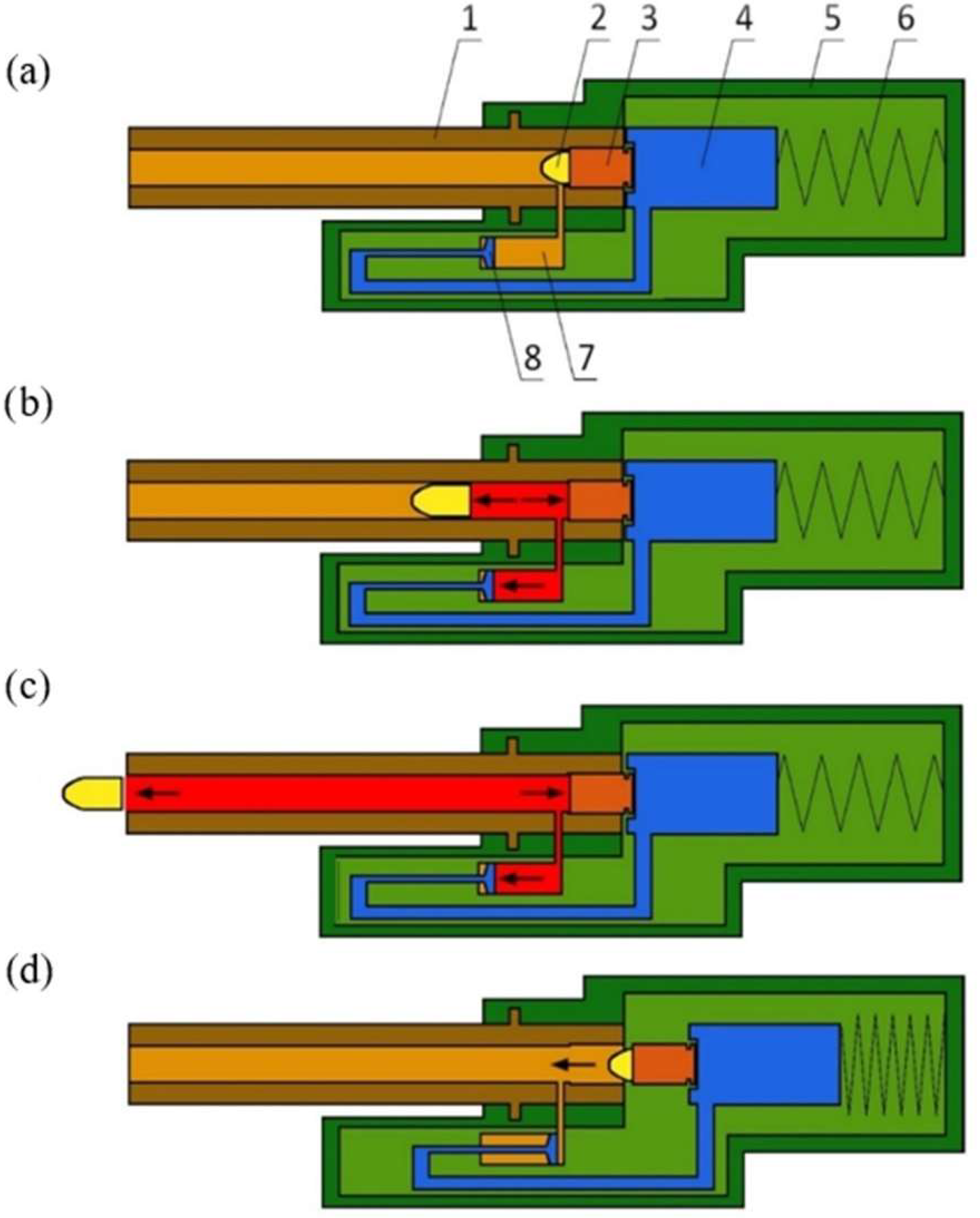
The description of the phenomena (the model of the interior ballistic) occurring in the system concerns a gas piston system in which some of the propellant gases are used to delay the recoiling assembly motion. When the shot is fired, the gases propel the projectile and, when it passes the gas port, some of the gases flow into the gas chamber and press on the front of the gas piston connected to the bolt. The scheme of the action of such a system is presented in Figure 1.

The phenomena described in the presented mathematical model apply to the operation that starts when the propellant is ignited and completed when the pressure in the system (barrel bore and gas chamber) has the same value as the ambient pressure. The model presented in study [7] required some improvements and, therefore—for the completeness of the description—an updated version is presented below. For the description of ballistic phenomena and kinematic equations occurring in the described model, the theory of internal ballistics and the thermodynamic approach proposed in a standardization document [6] was mainly used. It is important that the model takes into account the forces of interaction between: the projectile and barrel bore, the projectile and cartridge case, and the cartridge case and chamber [12,13,17,18]. However, due to the preliminary quality of the model, some simplifying assumptions were accepted to solve this problem. Despite some shortcomings in comparison with distributed parameters multiphase models [19] mainly based on finite volume approach—such as limited possibility of ignition process analysis—the lumped parameters models work well for short cartridge case systems [13], and—with some modifications—with long cartridge case solutions [20]. The main advantage of lumped parameters models is low computational cost of the simulation making use of numerical methods for ordinary differential equations [21].

For this kind of system of small arms operation, the equations are as follows (the nomenclature is presented at the end of the paper):

(a)

for the barrel bore:

the equation of the energy conservation:

-

when the pressure in the barrel bore is higher than the pressure in the gas chamber:

$$dU=dQ-d{E}_p-d{E}_{ra}-d{I}_g-d{I}_m$$

(1)

considering that:

$$dU=d\left[c_v\omega \left(\psi -\eta -\gamma \right)T\right]=c_v\omega \left[T\left(d\psi -d\eta -d\gamma \right)+\left(\psi -\eta -\gamma \right)dT\right]$$

$$dQ=d\left[c_v\left(T_1-T_0\right)\omega \psi \right]=q_s\omega d\psi$$

$$d{E}_p=\left(\frac{4{\pi }^2{I}_p}{{\eta }_b^2}+m+\frac{\omega }{3}\right)vdv+F_{r}vdt$$

$$d{E}_{ra}=MVdV+k_{rs}\left(x_0+L\right)Vdt$$

$$d{I}_g=c_{p}T\omega d\eta$$

$$d{I}_m=c_{p}T\omega d\gamma$$

the equation describing the balance of the energy is:

$$\begin{gathered} \frac{dT}{dt}=[\left(q_s-c_{v}T\right)\omega \frac{d\psi }{dt}-\theta c_{v}T\omega \left(\frac{d\eta }{dt}+\frac{d\gamma }{dt}\right)-\left(\frac{4{\pi }^2{I}_p}{{\eta }_b^2}+m+\frac{\omega }{3}\right)v\frac{dv}{dt} \\ -F_{r}v-MV\frac{dV}{dt}-k_{rs}\left(x_0+L\right)V\left]/\right[c_v\omega \left(\psi -\eta -\gamma \right)] \end{gathered}$$

(2)

-

when the pressure in the barrel bore is lower than the pressure in the gas chamber:

$$dU=dQ-d{E}_p-d{E}_{ra}-d{I}_g-d{I}_m$$

(3)

considering that:

$$dU=d\left[c_v\omega \left(\psi -\eta -\gamma \right)T\right]=c_v\omega \left[T\left(d\psi -d\eta -d\gamma \right)+\left(\psi -\eta -\gamma \right)dT\right]$$

$$dQ=d\left[c_v\left(T_1-T_0\right)\omega \psi \right]=q_s\omega d\psi$$

$$d{E}_p=\left(\frac{4{\pi }^2{I}_p}{{\eta }_b^2}+m+\frac{\omega }{3}\right)vdv+F_{r}vdt$$

$$d{E}_{ra}=MVdV+k_{rs}\left(x_0+L\right)Vdt$$

$$d{I}_g=c_p{T}_{gch}\omega d\eta$$

$$d{I}_m=c_{p}T\omega d\gamma$$

the equation describing the balance of the energy is:

$$\begin{gathered} \frac{dT}{dt}=[\left(q_s-c_{v}T\right)\omega \frac{d\psi }{dt}+\left(T-k{T}_{gch}\right)c_v\omega \frac{d\eta }{dt}-\theta c_{v}T\omega \frac{d\gamma }{dt} \\ -\left(\frac{4{\pi }^2{I}_p }{{\eta }_b^2}+m+\frac{\omega }{3}\right)v\frac{dv}{dt}-F_{r}v-MV\frac{dV}{dt}-k_{rs}\left(x_0+L\right)V\left]/\right[c_v\omega \left(\psi -\eta -\gamma \right)] \end{gathered}$$

(4)

-

equation defining the barrel bore propellant gas density:

$$\rho =\frac{\omega \left(\psi -\eta -\gamma \right)}{W_0-\frac{\omega }{\delta }\left(1-\psi \right)+s\left(l+L\right)}$$

(5)

-

equation of state of barrel bore propellant gas in the virial form:

$$p=RT\left(\rho +\beta {\rho }^2\right)$$

(6)

-

relative mass generation rate of gas produced by the combustion of the propellant:

$$\frac{d\psi }{dt}=\mathsf{\Gamma }\left(\psi \right)p_0{\left(\frac{p}{p_0}\right)}^{\propto }$$

(7)

-

equation defining the relative mass flow rate of the propellant gases flowing between the barrel bore and the gas chamber—when the pressure in the barrel bore is higher than the pressure in the gas chamber:

$$\mathrm{for}\frac{p_{gch}}{p}\le {\left(\frac{2}{k+1}\right)}^{\frac{k}{k-1}}$$

$$\frac{d\eta }{dt}=\frac{{\xi }_g{s}_{gp}}{\omega }{\left(\frac{2}{k+1}\right)}^{\frac{1}{k-1}}\sqrt{\frac{2k}{k+1}}\cdot \frac{p}{\sqrt{RT}}$$

(8)

$$\mathrm{for}\frac{p_{gch}}{p}>{\left(\frac{2}{k+1}\right)}^{\frac{k}{k-1}}$$

$$\frac{d\eta }{dt}=\frac{{\xi }_g{s}_{gp}}{\omega }\sqrt{\frac{2k}{k-1}\left[{\left(\frac{p_{gch}}{p}\right)}^{\frac{2}{k}}-{\left(\frac{p_{gch}}{p}\right)}^{\frac{k+1}{k}}\right]}\cdot \frac{p}{\sqrt{RT}}$$

(9)

-

equation defining the relative mass flow rate of the propellant gases flowing between the barrel bore and the gas chamber—when the pressure in the barrel bore is lower than the pressure in the gas chamber:

$$\mathrm{for}\frac{p}{p_{gch}}\le {\left(\frac{2}{k+1}\right)}^{\frac{k}{k-1}}$$

$$\frac{d\eta }{dt}=-\frac{{\xi }_g{s}_{gp}}{\omega }{\left(\frac{2}{k+1}\right)}^{\frac{1}{k-1}}\sqrt{\frac{2k}{k+1}}\cdot \frac{p_{gch}}{\sqrt{R{T}_{gch}}}$$

(10)

$$\mathrm{for}\frac{p}{p_{kg}}>{\left(\frac{2}{k+1}\right)}^{\frac{k}{k-1}}$$

$$\frac{d\eta }{dt}=-\frac{{\xi }_g{s}_{gp}}{\omega }\sqrt{\frac{2k}{k-1}\left[{\left(\frac{p}{p_{gch}}\right)}^{\frac{2}{k}}-{\left(\frac{p}{p_{gch}}\right)}^{\frac{k+1}{k}}\right]}\cdot \frac{p_{gch}}{\sqrt{R{T}_{gch}}}$$

(11)

-

equation defining the relative mass flow rate of the propellant gases that flows to the environment (when the bullet passed the muzzle of the barrel bore):

$$\frac{d\gamma }{dt}=\frac{{\xi }_{m}s}{\omega }{\left(\frac{2}{k+1}\right)}^{\frac{1}{k-1}}\sqrt{\frac{2k}{k+1}}·\frac{p}{\sqrt{RT}}$$

(12)

(b)

for the gas chamber:

the equation of the energy conservation:

-

when the pressure in the barrel bore is higher than the pressure in the gas chamber:

$$d{U}_{gch}=d{I}_g+d{E}_{gch}$$

(13)

considering that:

$$d{U}_{gch}=d\left[c_v\omega \eta T_{gch}\right]=c_v\omega \left[T_{gch}d\eta +\eta d{T}_{gch}\right]$$

$$d{I}_g=c_p\omega Td\eta$$

$$d{E}_{gch}=p_{gch}{s}_{gch}Vdt$$

the equation describing the balance of the energy is:

$$\frac{d{T}_{gch}}{dt}=\frac{\left(kT-T_{gch}\right)c_v\omega \frac{d\eta }{dt}+p_{gch}{s}_{gch}V}{c_v\omega \eta }$$

(14)

-

when the pressure in the barrel bore is lower than the pressure in the gas chamber:

$$d{U}_{gch}=d{I}_g+d{E}_{gch}$$

(15)

taking into account the following relations:

$$d{U}_{gch}=d\left[c_v\omega \eta T_{gch}\right]=c_v\omega \left[T_{gch}d\eta +\eta d{T}_{gch}\right]$$

(16)

$$d{I}_g=c_p\omega T_{gch}d\eta$$

(17)

$$d{E}_{gch}=p_{gch}{s}_{gch}Vdt$$

(18)

the equation describing the balance of the energy is:

$$\frac{d{T}_{gch}}{dt}=\frac{\theta c_v\omega T_{gch}\frac{d\eta }{dt}+p_{gch}{s}_{gch}V}{c_v\omega \eta }$$

(19)

-

equation defining the gas chamber propellant gas density:

$${\rho }_{gch}=\frac{\omega \eta }{W_{0gch}-s_{gch}L}$$

(20)

-

equation of the state of the gas chamber propellant gas:

$$p_{gch}=R{T}_{gch}\left({\rho }_{gch}+\beta {\rho }_{gch}^2\right)$$

(21)

(c)

other equations:

-

equation of the recoiling assembly motion:

$$\frac{dV}{dt}=\frac{ps-p_{gch}{s}_{gch}-F_{cc}-k_{rs}\left(x_0+L\right)}{M}$$

(22)

-

definition of the recoiling assembly velocity:

$$\frac{dL}{dt}=\mathrm{V}$$

(23)

-

equation of the bottom of the bullet pressure:

$$p_p=\frac{p+\frac{\omega }{3m}\frac{F_r}{s}}{1+\frac{\omega }{3m}}$$

(24)

-

equation of the bullet motion:

$$\frac{dv}{dt}=\frac{s{p}_p-F_r}{m}$$

(25)

-

definition of the bullet velocity:

$$\frac{dl}{dt}=v$$

(26)

Simulations were conducted for a system using 9 × 19 mm ammunition, since the designed laboratory stand will mainly be intended for such a cartridge.

Some of the significant results obtained or estimated in studies [12,13,22] were used in the model. These were, primarily, the course of the dynamic vivacity (and other characteristics of propellant charge) and the interaction forces between the projectile, barrel bore, cartridge case and chamber.

Table 1. Some weapon and ammunition parameters.

Parameter	Value
Bullet mass m (g)	8.00
Primary volume of cartridge case W0 (cm3)	0.57
Barrel length lm (m)	0.20
Correction factor of gas flowing through the gas port between barrel and gas chamber ξg	1
Correction factor of gas flowing out to the environment ξm	1

and

Table 2. Parameters of the powder in cartridge.

Parameter	Value
Powder mass ω (g)	0.340
Powder combustion heat qs (MJ/kg)	4.060
Force of the powder f (MJ/kg)	1.032
First virial coefficient β (m3/Mg)	1.585
Specific heats ratio k (-)	1.254
Density of the powder δ (kg/m3)	1330
Individual gas constant R (J/(K·kg))	360

show some parameters of the ammunition and weapon system used in the simulations.

Simulations were carried out using an original (own) program developed in MATLAB software, based on the above equations, definitions and data.

For the initial verification of the adopted model, some results (presented in

Table 3. Comparison of the results of preliminary verification model.

Parameter	Simulation Results	Reference Results [2]	Relative Discrepancy (%)
Maximum gas pressure in the barrel bore (MPa)	216.70	217.70	−0.46
Maximum velocity of the bullet (m/s)	386.90	380.70	1.63
Maximum velocity of the recoiling assembly (m/s)	5.19	5.16	0.58
Maximum barrel bore gas propellant density (kg/m3)	185.10	189.90	−2.53

) reached adequate weapon specifications (including bolt mass, barrel length and recoil spring parameters) and were compared with those obtained in study [2].

By comparing the results, it was concluded that the model seemed to be correct at this verification stage. Slight discrepancies may be caused due to the influence of some simplifications (especially concerning the ignition process or air resistance) or not taking into account the heat transfer process to the barrel [13,17], which is relatively negligible for fast-burning propellants applied in pistol ammunition [22]. However, detailed verification and validation of the model in the area concerning gas flow through the gas port, between the barrel bore and the gas chamber, and the associated impact on the action of the recoiling assembly, could be carried out following the experimental tests performed on a newly designed laboratory stand.

3. Results

The purpose of this analysis is to determine the impact of individual parameters of a weapon on the kinematic characteristic of the weapon system and to identify the parameters which have a negligible influence on the analyzed output parameter. Eliminating these parameters from the set of parameters analyzed in the experimental studies will reduce the time and costs of the testing. Moreover, determining the character of the influence of a given parameter (linear or nonlinear) will be useful in the creation of an experimental plan.

Therefore, if there is a mathematical model of the object (which was described in the previous section) and the results of simulations of the model are known, we can determine the relationship between the measured value (recoiling assembly velocity) and the value of the factor to give the function of the object. To accomplish this objective, the design of experimental methods are very useful.

Then, it is necessary to define the input parameters (factors) and their levels (from chosen ranges of the values), as well as to choose the experimental plan (linking the levels in treatments). The choice of ranges was influenced by limitations resulting from the design of the laboratory stand. For example, the minimum value of the gas port position was determined by the necessity to locate the hole in front of the forward edge of the cartridge case and the minimum value of the recoiling assembly mass results from the minimum size of the bolt necessary to mount it in the stand and install the components on it.

The number of factors (N) is 5 and these factors are: gas port location, gas port diameter, recoiling assembly mass, gas chamber initial volume and recoil spring stiffness. The values of the factors are shown in

Table 4. The values of the factors.

Parameter	k
	1	2	3	4	5
	Gas Port Location (mm)	Gas Port Diameter (mm)	Recoiling Assembly Mass (g)	Gas Chamber Initial Volume (cm3)	Recoil Spring Stiffness (N/m)
	lgp	dgp	Mra	W0gch	krs
xkmin—minimum not coded value of factor	7	1.0	280	1.5	500
xkmax—maximum not coded value of factor	37	1.8	380	2.5	1000
Δxk—mean value of factor (center of the plan)	22	1.4	330	2.0	750
Xkmin—minimum coded value of factor	−1
Xkmax—maximum coded value of factor	1

; for a better presentation of the plan, dimensionless values are also used.

The relation between coded and not coded values of factors is:

$$x_{ki}=\overline{x_k}+X_{ki}\Delta x_k$$

(27)

where:

i—serial number of a treatment,

x_ki/X_ki—not coded/coded level of factor x_k/X_k in the i-th treatment.

The complete plan can be used to provide all possible combinations of values of the factors. However, a major weakness in the complete plan is the high number of treatments; therefore, it is reasonable to apply the fractional plan, which consists of some selected treatments of the two-level complete plan [23]. The chosen treatments are sufficient to determine the coefficients of the linear function which approximates the response surface.

The first plan is a two-level fractional plan. The chosen contrast value is: I = 1. The number of treatments is 8 and two generating relations are used:

$$X_4=X_1{X}_2{X}_3$$

(28)

$$X_5=X_1{X}_2$$

(29)

The coded form of the plan is presented in

Table 5. The first two-level fractional plan.

N = 5; n = 25−2 = 8
i	X1	X2	X3	X4 = X1X2X3	X5 = X1X2
1	−1	−1	−1	−1	1
2	1	−1	−1	1	−1
3	−1	1	−1	1	−1
4	1	1	−1	−1	1
5	−1	−1	1	1	1
6	1	−1	1	−1	−1
7	−1	1	1	−1	−1
8	1	1	1	1	1

.

For the first fractional plan, the function describing the response surface is a linear function and is calculated as:

$$Z=6.814+0.644X_1-0.544X_2-1.040X_3+0.170X_4+0.137X_5$$

(30)

The values of the coefficients indicate that the influence of the factors X₁, X₂ and X₃ are significant; however, the influence of the factors X₄ and X₅ cannot be neglected.

Table 6. The results of simulations compared to the results approximated by the obtained function—for the first plan.

i	Maximum Recoiling Assembly Velocity (m/s)
	Simulation	Function
1	7.67	7.72
2	9.16	9.08
3	6.61	6.70
4	7.97	7.92
5	6.03	5.98
6	6.56	6.65
7	4.37	4.28
8	6.13	6.18
Mean	6.81	6.81

presents the results of simulations compared with the results approximated by the obtained function.

Comparing the results obtained from the numerical simulation and those approximated by the linear function, the differences between these results were found to be slight, with a maximum difference of 0.09 (approximately 2.05%). Therefore, it should be considered that the function of the object was calculated correctly. However, in order to be sure that the object can be considered to be linear (within the assumed range of parameters), one must perform the analysis for the two-level fractional plan in which one of the contrasts is equal to −1.

Therefore, for the second two-level fractional plan, the contrast for the fifth factor was changed to I = (−1) and the other values remained unchanged. Furthermore, for this plan, the calculation of values using a linear function with coefficients calculated for the first plan was carried out—the results are shown in the ‘Approximation’ column in

Table 7. The results of simulation compared to the results approximated by the obtained function—for the second plan.

i	Maximum Recoiling Assembly Velocity (m/s)
	Simulation	Function	Approximation
1	7.76	7.81	7.45
2	9.04	8.96	9.35
3	6.52	6.61	6.97
4	8.07	8.01	7.65
5	6.11	6.06	5.71
6	6.48	6.57	6.93
7	4.30	4.22	4.55
8	6.20	6.26	5.91
Mean	6.81	6.81	6.81

. The function describing the response surface was calculated as:

$$Z=6.811+0.637X_1-0.537X_2-1.037X_3+0.158X_4-0.224X_5$$

(31)

Although the function gives a good estimation of the results from simulations, the maximum difference value is 0.09 (about 2.01%), the approximated values are significantly different. The recoiling assembly velocity values for the second plan, according to the coefficients determined for the first plan, compared to the values from the simulation show a discrepancy of 5.7%. It is also puzzling that the coefficient at X₅ has changed its sign. Values of coefficients at other factors have not changed considerably. These findings may indicate that the influence of the parameters is not linear.

The third plan is formed by the connection of the first and second two-level fractional plan and so the number of treatments is 16 (

Table 8. The results of simulation (for plan 3) compared with the results approximated by the obtained function (for plan 1, 2 and 3).

i	Maximum Recoiling Assembly Velocity (m/s)
	Simulation	Function—Plan 3	Function—Plan 1	Function—Plan 2
1	7.67	7.54	7.72	-
2	9.16	9.24	9.08	-
3	6.61	6.88	6.70	-
4	7.97	7.74	7.92	-
5	6.03	5.79	5.98	-
6	6.56	6.83	6.65	-
7	4.37	4.47	4.28	-
8	6.13	5.99	6.18	-
9	7.76	7.63	-	7.81
10	9.04	9.15	-	8.96
11	6.52	6.79	-	6.61
12	8.07	7.83	-	8.01
13	6.11	5.88	-	6.06
14	6.48	6.75	-	6.57
15	4.30	4.38	-	4.22
16	6.20	6.08	-	6.26
Mean	6.81	6.81	6.81	6.81

).

For the third plan, the function describing the response surface was calculated as:

$$Z=6.812+0.641X_1-0.540X_2-1.039X_3+0.164X_4-0.044X_5$$

(32)

For the third plan, the maximum difference value is 0.24 (about 4.13%). The functions of the object obtained for all three plans are summarized in

Table 9. The functions of the object obtained for all three plans.

Plan	Function of the Object
Plan 1	$Z=6.814+0.644X_1-0.544X_2-1.040X_3+0.170X_4+0.137X_5$
Plan 2	$Z=6.811+0.637X_1-0.537X_2-1.037X_3+0.158X_4-0.224X_5$
Plan 3	$Z=6.812+0.641X_1-0.540X_2-1.039X_3+0.164X_4-0.044X_5$

.

Based on the obtained functions, it can be concluded that the coefficient values for plan 3 are intermediate between those calculated for plan 1 and plan 2. However, the coefficient at the fifth factor (the recoil spring stiffness) is very small, which may indicate the possibility of neglecting the influence of this parameter, or the influence of some nonlinearities.

To verify the hypothesis, computations were carried out for the Bi plan [23] and the results were approximated by a quadratic function. The plan consists of a core, in the form of a two-level fractional plan (or, optionally, a two-level complete plan) and star points with the star arm equal to 1. The center of the plan is not part of this plan. For five factors, the core of the plan comprised a minimum of 2⁵⁻¹ treatments. Therefore, the entire plan included 26 treatments (16 for the core and 10 star points), summarized in

Table 10. The results of simulation compared to the results approximated by the obtained function for the Bi plan.

i	Maximum Recoiling Assembly Velocity (m/s)
	Simulation	Function
1	7.67	7.66
2	8.92	8.91
3	5.93	5.94
4	7.97	7.99
5	5.72	5.70
6	6.48	6.46
7	4.30	4.31
8	5.94	5.94
9	8.30	8.30
10	9.04	9.03
11	6.52	6.54
12	8.43	8.45
13	6.03	6.02
14	6.75	6.73
15	4.87	4.87
16	6.13	6.13
17	6.02	6.02
18	7.30	7.30
19	7.40	7.49
20	6.50	6.41
21	8.17	8.13
22	6.01	6.05
23	6.71	6.70
24	7.08	7.09
25	6.97	6.97
26	6.89	6.88
Mean	6.85	6.85

.

For the Bi plan, the function describing the response surface is:

$$\begin{array}{cc}\hfill Z=& 6.929+0.644X_1-0.540X_2-1.040X_3+0.196X_4-0.044X_5-0.269X_1{}^2\hfill \\ & +0.022X_2{}^2+0.163X_3{}^2-0.032X_4{}^2-0.001X_5{}^2+0.211X_1{X}_2\hfill \\ & -0.099X_1{X}_3-0.066X_1{X}_4-0.008X_1{X}_5+0.083X_2{X}_3\hfill \\ & +0.029X_2{X}_4+0.015X_2{X}_5-0.029X_3{X}_4+0.003X_3{X}_5\hfill \\ & -0.035X_4{X}_5\hfill \end{array}$$

(33)

and the maximum relative error is 1.36%. Moreover, the values of the response for mean values of factors (for the center of the plan) were calculated using the obtained functions, and summarized in

Table 11. The results of simulation compared to the results approximated by the obtained function for the center of the plan.

Maximum Recoiling Assembly Velocity for the Center of the Plan (m/s)
Simulation (MATLAB)	Plan 1	Plan 2	Plan 3	Plan Bi
6.93	6.81	6.81	6.81	6.93
Relative error:	1.73%	1.73%	1.73%	<0.01%

. Thus, it is possible to check the correctness of the approximation, as well as to represent the graphs more accurately.

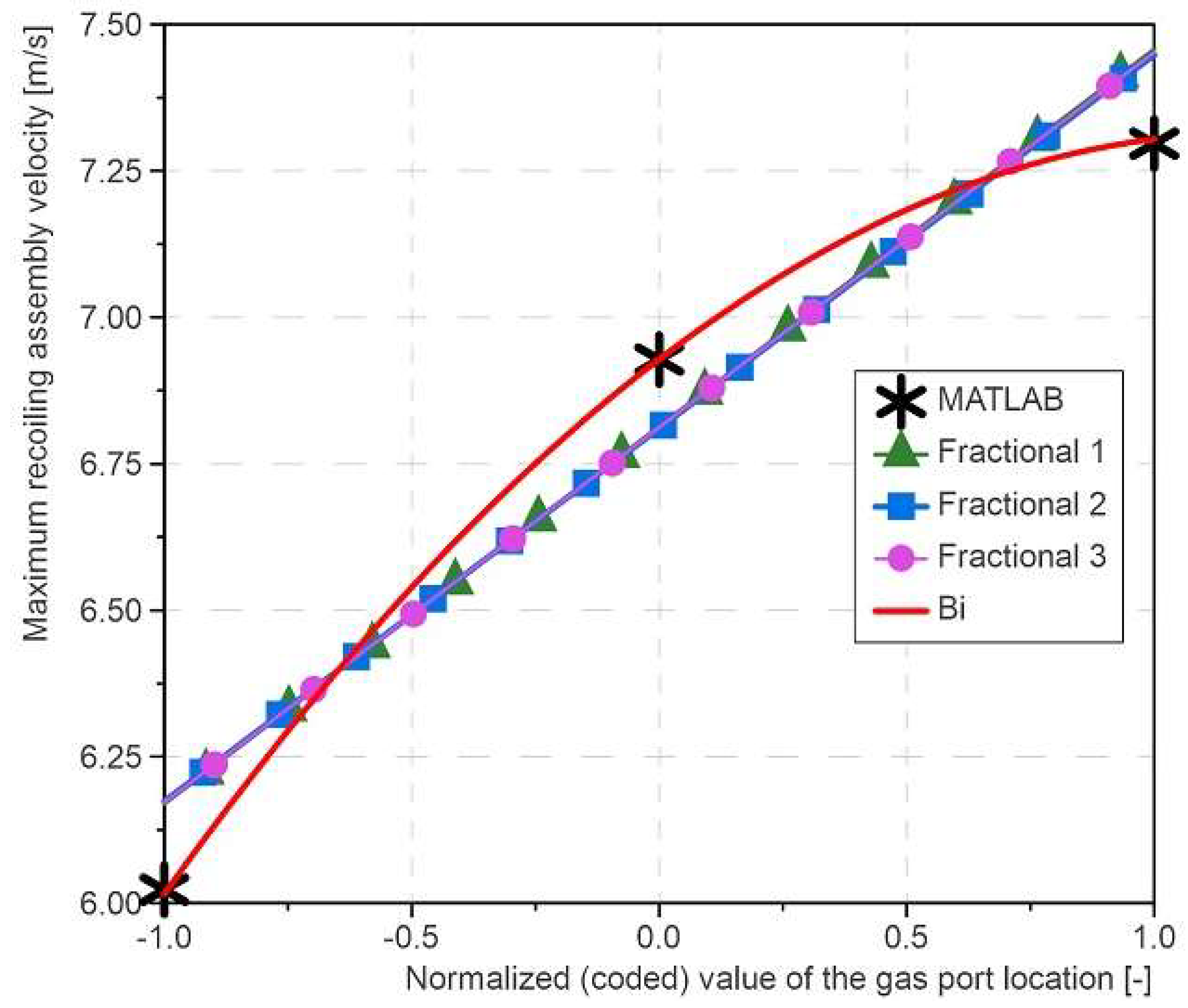
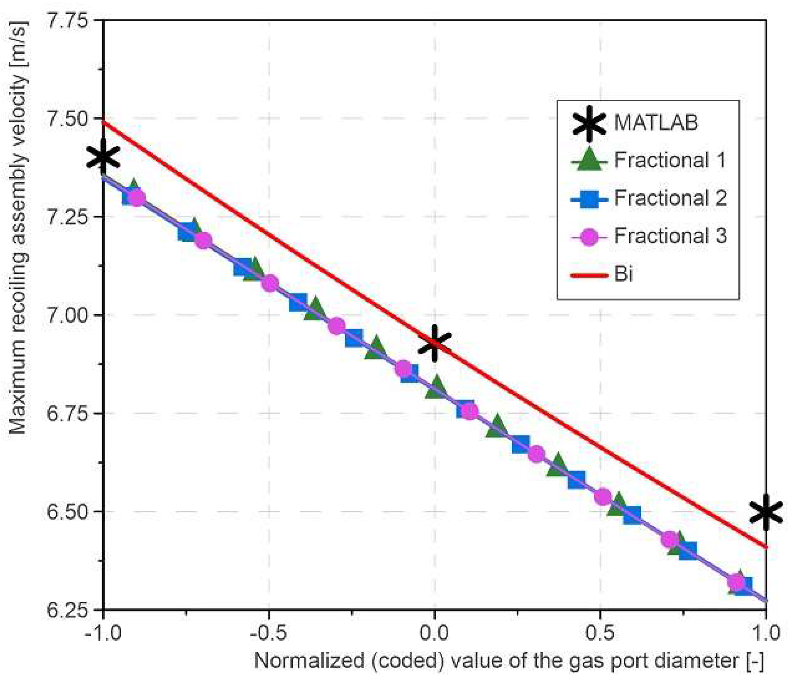
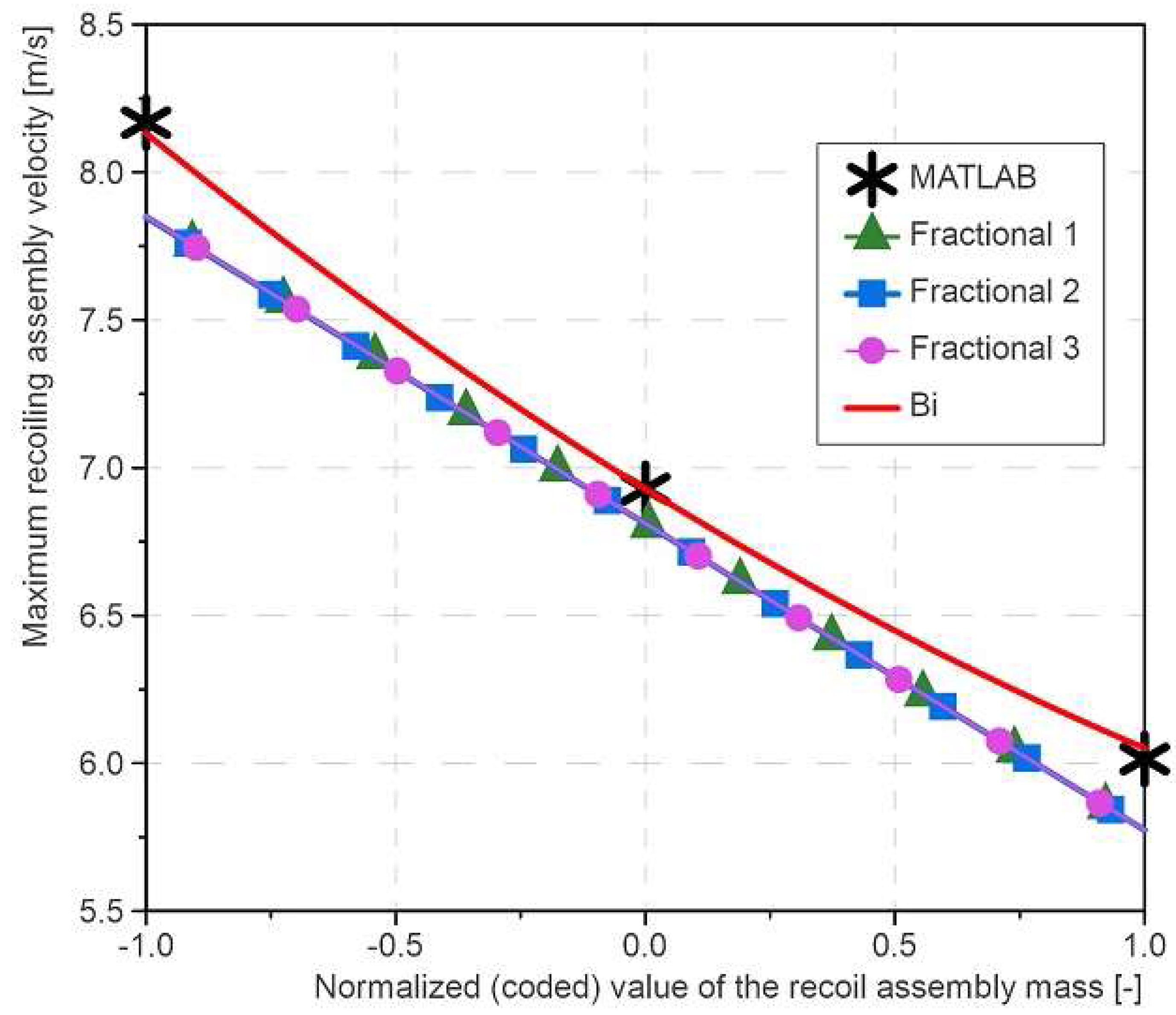
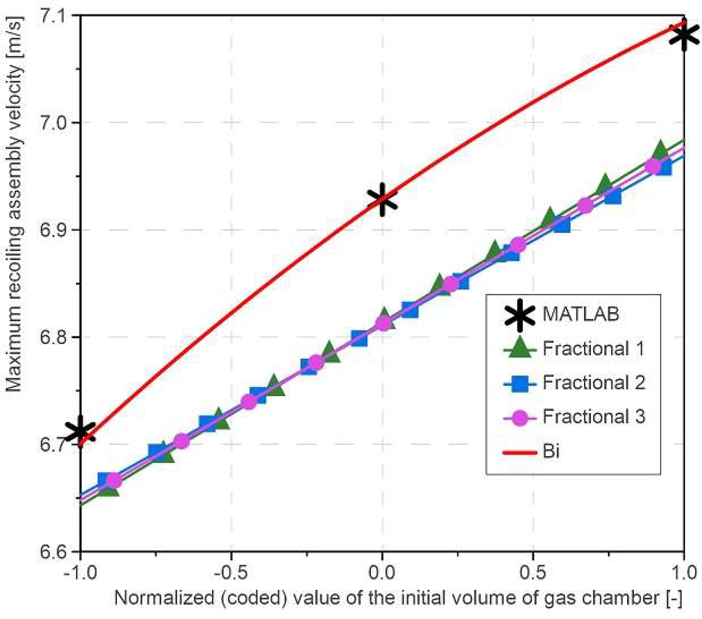
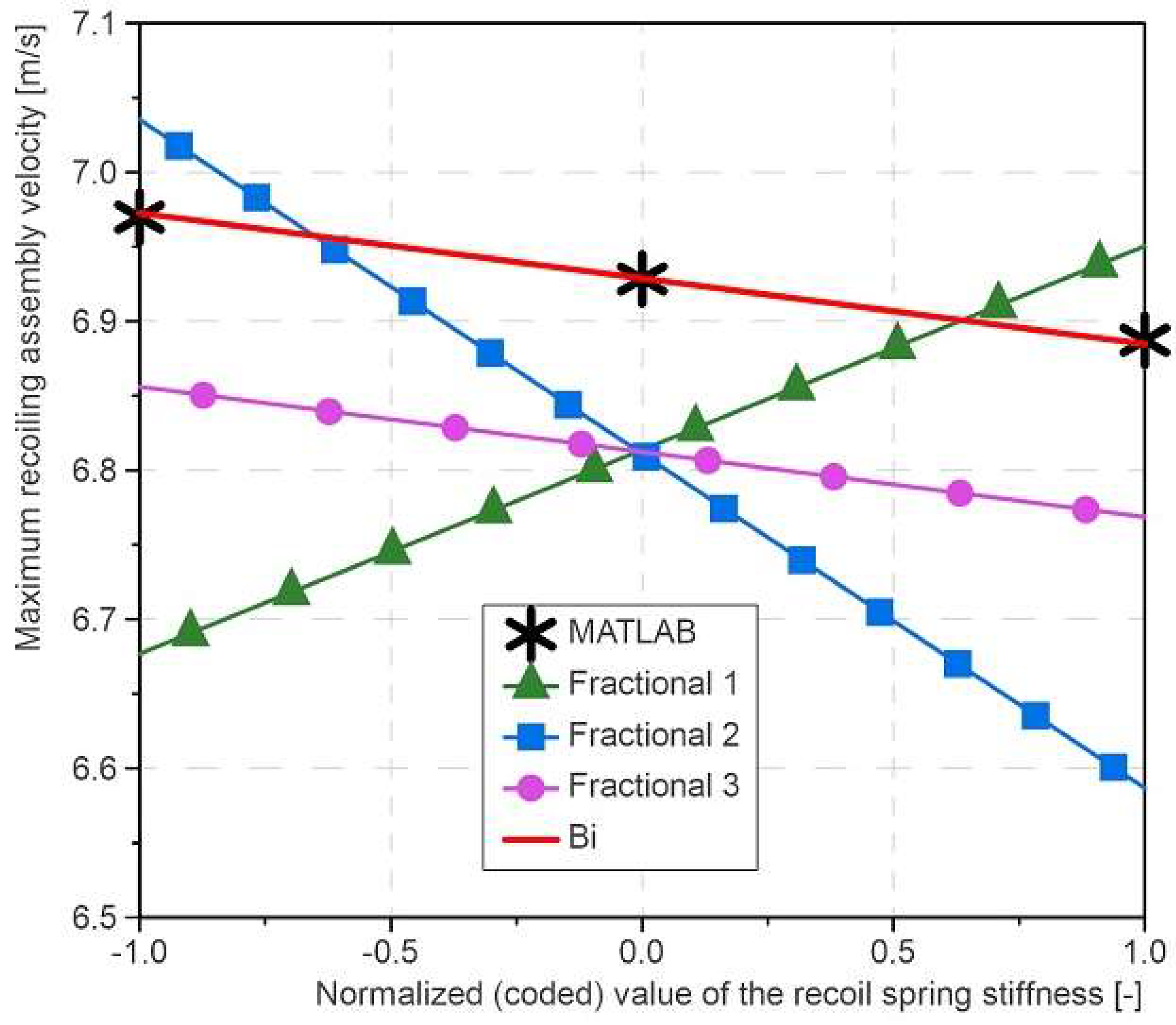
Figure 2, Figure 3, Figure 4, Figure 5 and Figure 6 show the functions of the object obtained for each plan when only one factor is changed and other factors have values for the center of the plan. In addition, the graphs indicate (with stars) the values of the recoil assembly velocity obtained from the simulation for the limiting values of the factor and for the center of the plan. In the first three graphs, the functions of plan 3 almost overlap with those of plan 1 and 2, which is why they are faintly visible.

4. Discussion

By analyzing the obtained results and graphs, it can be concluded that the dependence of the recoiling assembly velocity on the factors is not linear. However, the calculated and presented quadratic function approximation gives a very close estimation of the simulation results. The function obtained from plan Bi allows us to state that the strongest influences on the results are (in decreasing order): the recoiling assembly mass, the gas port location and the gas port diameter. Theoretically, increasing the recoiling assembly mass is the easiest way to reduce the recoiling assembly velocity (such a solution is characteristic of simple blowback weapons). The consequence of this is to primarily increase the weight of the entire firearm. Therefore, it was very significant to verify the influence of the other factors.

It is significant that the expected result was that the most advantageous solution—from the point of view of recoiling assembly braking—and is the shortest distance (for the starting position of the bullet—when the cartridge is in the chamber) of the bullet to the gas port. The minimum value of this distance is forced by the cartridge case length. Then, the largest coefficient in the quadratic function has this factor. This is justified by the fact that the location of the gas port, in close proximity to the front edge of the cartridge case, causes the propellant gases to have energy, which results in a significant decrease in recoiling assembly velocity. As the port is moved toward the muzzle of the barrel, much less gas flows into the gas chamber, and so the deceleration is increasingly negligible. This is largely due to the characteristics of pistol ammunition, in which a propellant charge is burned very dynamically.

As can be seen, the recoil spring stiffness has the least influence; it is practically insignificant in the assumed range (even though the maximum value is twice the minimum). The research reported in study [24] also found negligibly small effects of this factor on recoiling assembly velocity; these results were for gas-operated small arms. Therefore, it was concluded that its impact would not be further investigated. This is very important when considering the cost and time-consuming nature of research.

5. Conclusions

Considering the presented analysis results, the following conclusions can be made:

• Preliminary estimation of the influence of the parameters allows the determination of the parameters of the newly designed laboratory stand and it also allows rejection of one of the factors as insignificant—recoil spring stiffness.
• The linear function is not an accurate approximation of the results, while a quadratic function is. This means that, in the experimental investigations, only three levels of the values of the factors are sufficient. Based on the results of the analysis, we chose the plan Bi for the design of future experiments. The experimental stand was designed in such a way that it will enable us to perform measurements in accordance with this plan.
• The application of design of experimental methods enables us to plan the research clearly and properly, to present it in an interesting form and to obtain results that are more difficult to obtain without knowledge of these tools.

References

1. Carlucci, D.E.; Jacobson, S.S. Ballistics: Theory and Design of Guns and Ammunition, 3rd ed.; CRC Press: Boca Raton, FL, USA, 2018. [Google Scholar]
2. Morawski, M.; Zahor, M. Delayed Blowback Operation Firearms in the Small Arms Classification. Probl. Mechatron. Armament Aviat. Saf. Eng. 2021, 12, 101–118. [Google Scholar] [CrossRef]
3. Fikus, B. Development and Validation of Blowback Small Arms Theoretical Model. Ph.D. Thesis, Military University of Technology, Warsaw, Poland, 2018. (In Polish). [Google Scholar]
4. Radomska, A.; Radomski, M. Solution of Main Problem of Interior Ballistics of the Pistol Heckler i Koch 9 mm Para. Probl. Tech. Uzbroj. Radiolokacji 1984, 34, 37–53. (In Polish) [Google Scholar]
5. Dannecker, P. Verschlussysteme Von Feuerwaffen; DWJ: Blaufelden, Germany, 2016. (In German) [Google Scholar]
6. STANAG 4367 Land. In Thermodynamic Interior Ballistic Model with Global Parameters, 2nd ed.; Military Agency for Standardization: Brussels, Belgium, 2000.
7. Fikus, B.; Morawski, M.; Woźniak, R. Formulation of interior ballistic model of gas delayed blowback operation firearm. In Proceedings of the International Scientific Conference—Defense Technologies DefTech 2021, Shumen, Bulgaria, 6–8 October 2021. [Google Scholar]
8. Fikus, B.; Trębiński, R. Numerical simulation of submachine gun operation cycle. In Proceedings of the International Scientific Conference—Defense Technologies DefTech 2020; Faculty of Artillery, Air Defense and Communication and Information Systems: Shumen, Bulgaria; 2020. [Google Scholar]
9. Szupieńko, D.; Woźniak, R. Preliminary Physical and Mathematical Model of the Recoil Operated Firearm within the Bolt Recoil Period. Probl. Mechatron. Armament Aviat. Saf. Eng. 2021, 12, 59–74. [Google Scholar] [CrossRef]
10. Leśnik, G.; Surma, Z.; Torecki, S.; Woźniak, R. Termodynamiczny model działania broni z odprowadzeniem gazów prochowych w okresie napędzania suwadła. Biul. WAT 2009, 3, 193–209. [Google Scholar]
11. Tien, V.D.; Macko, M.; Procházka, S.; Bien, V.V. Mathematical Model of a Gas-Operated Machine Gun. Adv. Mil. Technol. 2022, 17, 63–77. [Google Scholar] [CrossRef]
12. Fikus, B.; Płatek, P.; Surma, Z.; Sarzyński, M.; Trębiński, R. Preliminary numerical and experimental investigations of 9 mm pistol bullet and barrel interaction. In Proceedings of the 31st International Symposium on Ballistics, Hyderabad, India, 4–8 November 2019; Saraswat, V.K., Reddy, G.S., Woodley, C., Eds.; Destech Publications Inc.: Lancaster, PA, USA, 2019. [Google Scholar]
13. Fikus, B.; Surma, Z.; Trębiński, R. Preliminary Application Correctness Assessment of Physical Burning Law in Interior Ballistics Phenomena Modeling in Small-Caliber Guns. In Proceedings of the 31st International Symposium on Ballistics, Hyderabad, India, 4–8 November 2019; Saraswat, V.K., Reddy, G.S., Woodley, C., Eds.; Destech Publications Inc.: Lancaster, PA, USA, 2019. [Google Scholar]
14. Țîțu, A.M.; Sandu, A.V.; Pop, A.B.; Țîțu, S.; Frățilă, D.N.; Ceocea, C.; Boroiu, A. Design of Experiment in the Milling Process of Aluminum Alloys in the Aerospace Industry. Appl. Sci. 2020, 10, 6951. [Google Scholar] [CrossRef]
15. Hsueh, K.; Lin, T.; Lee, M.; Hsiao, Y.; Gu, Y. Design of Experiments for Modeling of Fermentation Process Characterization in Biological Drug Production. Processes 2022, 10, 237. [Google Scholar] [CrossRef]
16. Esfe, M.H.; Motallebi, S.M.; Toghraieb, D. A novel experimental and statistical study on ethylene glycol-based nanofluid enriched by MWCNT and CuO nanoparticles. Ann. Nucl. Energy 2022, 177, 109283. [Google Scholar] [CrossRef]
17. Fikus, B.; Dorochowicz, A.; Surma, Z.; Kijewski, J.; Leciejewski, Z.; Michalski, J.; Trębiński, R. Investigations of Middle-Caliber Anti-Aircraft Cannon Interior Ballistics including Heat Transfer Problem in Estimation of Critical Burst Length. Processes 2022, 10, 607. [Google Scholar] [CrossRef]
18. Badurowicz, P.; Kupidura, P.; Fikus, B. Numerical and Experimental Investigation of a Short Recoil Operated Weapon and Impact of Construction Characteristics on its Operation Cycle. Def. Sci. J. 2022, 72, 326–333. [Google Scholar] [CrossRef]
19. Otón-Martínez, R.A.; Velasco, F.J.S.; Nicolás-Pérez, F.; García-Cascales, J.R.; Mur-Sanz de Galdeano, R. Three-Dimensional Numerical Modeling of Internal Ballistics for Solid Propellant Combinations. Mathematics 2021, 9, 2714. [Google Scholar] [CrossRef]
20. Trębiński, R.; Leciejewski, Z.; Surma, Z.; Fikus, B.; Szupieńko, D. Identification of experimental form function using lumped parameters interior ballistics model. In Proceedings of the 32nd International Symposium, Reno, Nevada, 9–13 May 2022; Manning Thelma, G., Rickert Frederick, C., II, Eds.; DEStech Publications: Lancaster, PA, USA, 2022; pp. 421–432, ISBN 978-1-60595-689-3. [Google Scholar]
21. Björck, A.; Dahlquist, G. Numerical Methods; PWN: Warsaw, Poland, 1987. (In Polish) [Google Scholar]
22. Trębiński, R.; Fikus, B.; Surma, Z. Investigations of Ballistic Characteristics of N340 Propellant. Probl. Mechatron. Armament Aviat. Saf. Eng. 2017, 8, 9–22. [Google Scholar] [CrossRef]
23. Polański, Z. Design of Experiments in Technical Science; PWN: Warsaw, Poland, 1984. (In Polish) [Google Scholar]
24. Kijewski, J.; Leśnik, G.; Pac, M. Theoretical and Experimental Tests of Influence of Recoil Springs Stiffness on Slide Velocity of Gas-Operated Weapon (in Polish). Probl. Mechatron. Armament Aviat. Saf. Eng. 2014, 5, 107–118. [Google Scholar] [CrossRef]
Figure 1. Scheme of action of gas-delayed blowback operation firearm: 1—barrel, 2—projectile, 3—cartridge case, 4—bolt (recoiling assembly), 5—upper receiver, 6—recoil spring, 7—gas chamber, 8—gas piston. (a) the initial position: round in the chamber, bolt in forward position and closed barrel; (b) the shot is initiated, projectile is moving in the barrel, gases flowing through the gas port to the gas chamber (and/or from the gas chamber to the barrel bore), gases are pressing on the breech face (bolt is accelerated) and on the front of the gas piston (bolt is decelerated); (c) the projectile is out of the barrel (has passed the muzzle), gases are pressing on the breech face (bolt is accelerated) and on the gas piston (bolt is decelerated); (d) bolt in the rear position, the next round is chambering.
Applsci 12 12216 g001
Figure 2. Diagram of the maximum recoiling assembly velocity as a function of the normalized (coded) value of the gas port location.
Applsci 12 12216 g002
Figure 3. Diagram of the maximum recoiling assembly velocity as a function of the normalized (coded) value of the gas port diameter.
Applsci 12 12216 g003
Figure 4. Diagram of the maximum recoiling assembly velocity as a function of the normalized (coded) value of the recoiling assembly mass.
Applsci 12 12216 g004
Figure 5. Diagram of the maximum recoiling assembly velocity as a function of the normalized (coded) value of the initial volume of the gas chamber.
Applsci 12 12216 g005
Figure 6. Diagram of the maximum recoiling assembly velocity as a function of the normalized (coded) value of the recoil spring stiffness.
Applsci 12 12216 g006