Article

Prostate Gleason Score Detection by Calibrated Machine Learning Classification through Radiomic Features

Department of Medicine and Health Sciences “Vincenzo Tiberio”, University of Molise, 86100 Campobasso, Italy
*
Author to whom correspondence should be addressed.
Appl. Sci. 2022, 12(23), 11900; https://doi.org/10.3390/app122311900
Submission received: 14 September 2022 / Revised: 16 November 2022 / Accepted: 18 November 2022 / Published: 22 November 2022
(This article belongs to the Special Issue New Applications of Deep Learning in Health Monitoring Systems)

Abstract

:
The Gleason score was originally formulated to represent the heterogeneity of prostate cancer and helps to stratify the risk of patients affected by this tumor. The Gleason score assigning represents an on H&E stain task performed by pathologists upon histopathological examination of needle biopsies or surgical specimens. In this paper, we propose an approach focused on the automatic Gleason score classification. We exploit a set of 18 radiomic features. The radiomic feature set is directly obtainable from segmented magnetic resonance images. We build several models considering supervised machine learning techniques, obtaining with the RandomForest classification algorithm a precision ranging from 0.803 to 0.888 and a recall from to 0.873 to 0.899. Moreover, with the aim to increase the never seen instance detection, we exploit the sigmoid calibration to better tune the built model.

1. Introduction and Related Work

In 2018, there were 1,276,106 new cases of prostate cancer, making it the second most common disease in males globally (after lung cancer). Additionally, 358,989 men died from prostate cancer, accounting for 3.8% of all deaths in men from cancer [1].
The survival of patients with prostate cancer, not considering mortality from other causes, is currently at about 92%, five years after diagnosis, and these figures are in constant and significant growth. The diagnostic anticipation and the progressive diffusion of opportunistic screening by PSA testing are the main factors correlated to this temporal trend [2,3]. The “opportunistic” use of PSA is endorsed by the available evidence suggesting that organized PSA-based screening could, at best, lead to a minimal reduction in cancer-specific mortality. Still, it would not lead to a reduction in global mortality. At the same time, it would undoubtedly cause adverse collateral effects due to overdiagnosis [4].
Prostate adenocarcinoma originates in the peripheral portion of the gland in over 70% of cases, and it is, therefore, often appreciable in rectal examination. In addition, 20% of neoplasms arise in the transitional anteromedial part of the organ. At the same time, the central area is typical of prostatic hyperplasia and is the primary site of only 5% of neoplasms. Prostate cancers are mostly multifocal and heterogeneous in grade and histological appearance [5,6]. The reference classification for identifying the histotypes of prostate cancer is that indicated by the World Health Organization (WHO) in 2016 [7]. The original Gleason grading system (from 1 to 5 degrees) and the Gleason score (with a score from 2 to 10), created to represent the heterogeneity of prostate neoplasms, were modified in 2005 and 2014 by the International Society of Urological Pathology (ISUP). The score is assigned based on the most represented structural aspect (primary grade) and the second most represented or at the highest of the least represented (secondary degree) in the neoplasm. Up to date, the minimum diagnosable score is 6 ( 3 + 3 ). The essential histological characteristics of Gleason can be summarized as follows: (i) 3 + 3 : there are individual discrete well-formed glands (this category is representing the less aggressive one); (ii) 3 + 4 : mainly composed by well-formed glands, but a small component of poorly formed, fused and or cribriform glands appears; (iii) 4 + 3 : mainly composed by poorly formed, fused and/or cribriform glands with lesser well-formed glands; (iv) 4 + 4 : usually composed only by poorly formed, fused and/or cribriform glands; from this score, the cancer is considered as aggressive [8,9,10].
Prostate cancer diagnoses are essentially based on rectal exploration, PSA dosage, imaging techniques, and histological reports of prostatic needle biopsies. Multiparametric MRI plays a fundamental role in detecting prostate cancer in patients with clinical suspicion: the now consolidated multiparametric protocol, which includes T2-weighted, T1-weighted anatomical sequences in perfusion (Dynamic Contrast-Enhanced Magnetic Resonance Imaging, DCE-MRI) and diffusion weighting (Diffusion-Weighted Imaging, DWI), can provide a combination of anatomical, biological, and functional information necessary for a more precise definition of suspicious lesions. The indication to perform a prostate biopsy for diagnosis by histopathological examination is currently being formulated based on clinical and/or laboratory suspicion (pathological changes in biomarkers) and/or positive outcome of the multiparametric MRI [11]. Nowadays, multiparametric MRI, through its morphological T2 sequences, DWI, and functional MR modalities (MRSI), achieves the highest sensitivity (0.84) and negative predictive value (0.93) in prostate cancer detection [12]. The prostate is typically assigned a radiological score on MRI multiparametric images, which indicates the likelihood of a clinically significant cancer of the gland: this score is called PI-RADS [13]. In patients with a moderate/high PI-RADs score or increased PSA > 10, a prostate biopsy to confirm the diagnostic suspect might be suggested [14]. The information reported in the pathology report is extremely important to define the patient’s therapeutic perspectives and prognosis. In the case of biopsy specimens positive for cancer, the pathologist assigns an individual Gleason score for each needle biopsy specimen, taking into account the site of collection of each of them. In order to give patients a favorable prognosis, early detection is crucial to avoid the disease progression and the involvement of other organs [15].
In recent years, radiomic has been emerging as a new research field in which medical images, for instance, magnetic resonance imaging (MRIs), are converted into numbers [16]. Radiomic has the potential to uncover disease characteristics that fail to be recognised by the naked human eye; in this way, it is possible to provide valuable information for personalised therapy [17].
Machine learning methods demonstrated the ability to learn feature representations automatically from numeric data under analysis. These features are considered to automatically build models with well-known classification algorithms [18]. In detail, supervised machine learning algorithms can be exploited in order to build predictive models starting from labeled radiomic characteristics.
In this paper, a method that aims to detect the 3 + 4 , 4 + 3 and 4 + 4 prostate cancer Gleason score is provided. We consider a set of radiomic features and, through supervised machine learning classification techniques, we label MRIs as related to 3 + 4 , 4 + 3 or 4 + 4 Gleason score.
With regard to the current state of the art, machine learning techniques were explored by researchers in this field. For instance, Huang and colleagues [19] consider deep learning to discriminate between low- and high-grade localized tumors. They obtain an accuracy equal to 70%. They do not provide details about the considered architecture, anyway discriminating between low-grade and high-grade localized tumors. Differently, the method we propose is able to detect between the low and the high-grade cancers (for instance, the ones labelled with the 3 + 4 and the 4 + 3 Gleason scores).
The authors in [20] experiment with three different state-of-the-art supervised machine learning algorithms with the aim to identify several types of cancer using gene expression as a feature vector. With regard to prostate cancer, they obtain the following results in terms of accuracy: 67.65%, 73.53%, and 67.65%, respectively, using the C4.5 decision tree, bagged algorithms.
The main contribution of this paper is the detection of the 3 + 4 , 4 + 3 and 4 + 4 Gleason scores exploiting calibrated machine learning through a set of radiomic features. The paper proceeds as follows: the next section presents the proposed method, Section 3 discusses the experimental analysis results, and conclusions and future works are drawn in the last section.

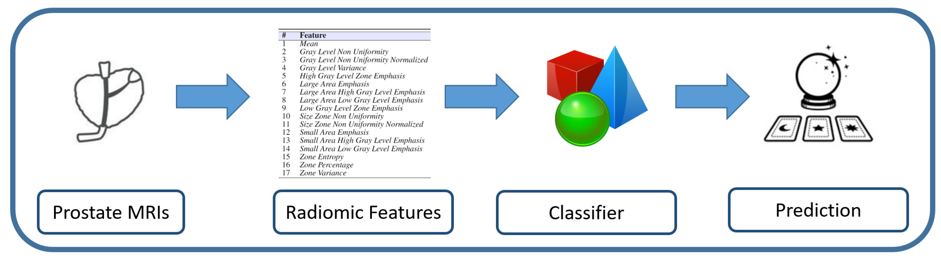
2. Materials and Methods

We present the method we designed for prostate cancer Gleason score detection by applying supervised machine learning. We detect Gleason score prostate cancer from prostate medical images i.e., MRIs.
As stated in the Introduction, in order to evaluate the efficacy of the proposed approach, a dataset freely available for research purposes is exploited: https://wiki.cancerimagingarchive.net/display/Public/PROSTATE-DIAGNOSIS (accessed on 18 November 2022). The dataset is composed by multiparametric MRI images of patients affected by prostate cancers, confirmed by a pathologist; in particular, T1- and T2-weighted MRIs are considered. The medical images were acquired by exploiting a 1.5 T Philips Achieva by combined surface and endorectal coil, including dynamic contrast-enhanced images obtained prior to, during and after I.V. administration of 0.1 mmol/kg body weight of Gadolinium-DTPA (pentetic acid).
The dataset contains the segmentation (i.e., the ROI), pathology biopsy and excised gland tissue reports. Moreover, in the dataset for each medical examination, there is a radiology report: the radiomic features are extracted on the ROI area.
We consider a total of 670 MRIs: in particular, 338 MRIs were marked by pathologists with a 3 + 4 Gleason Score, 173 were marked by pathologists with a Gleason Score equal to 4 + 3 , while 159 were marked by pathologists with a Gleason Score equal to 4 + 4 .
With regard to the classification analysis, we developed a series of Python scripts invoking the scikit-learn (https://scikit-learn.org/stable/ accessed on 18 November 2022) library, a machine learning library for the Python programming language network. The radiomic features have been extracted using PyRadiomics (https://pyradiomics.readthedocs.io/en/latest/ accessed on 18 November 2022), a Python package aimed at gathering a set of radiomic features directly from MRIs [21].
To this aim, we consider 18 different radiomic features related to three different categories:
  • First Order (FO): this category is related to the voxel distribution of the intensities within the ROI (i.e., the region of interest that in this study is represented by the areas interested by the cancer). We extract 1 feature belonging to the FO category;
  • Gray Level Run Length Matrix (GLRLM): the features related to this category consider the grey level run length matrix, aiming to give the size of (homogeneous) runs for each grey level. In addition, in this category, 1 feature is considered;
  • Gray Level Size Zone Matrix (GLSZM): the features related to the GLSZM category are aimed at quantifying the gray level zones in a medical image under analysis. With the gray level zone, we refer to a zone defined as the number of (connected) voxels sharing the same gray level intensity. Sixteen different features are considered from this category.
The considered features with the relative category are shown in Table 1.
The aim of the proposed experiment is to understand if the exploited radiomic features are effective at automatically discerning between 3 + 4 , 4 + 3 and 4 + 4 Gleason scores by verifying if the radiomic feature vector composed of 18 features is able to detect the Gleason Score from unseen MRIs. The classification is performed by exploiting four different classification algorithms with the radiomic features.
We design an evaluation composed of three different steps: the first one is a statistics evaluation, where we compare the populations of MRIs related to different Gleason scores: the aim is to understand whether the radiomics features exhibit different values when extracted from MRIs related to Gleason score; the second step is the hypotheses testing that is related to understanding whether the features exhibit different distributions of the MRIs; the third step is a classification analysis which aims to understand if the exploited radiomic features are able to rightly discern different unknown MRIs related to different Gleason scores.
For the statistics evaluation, we compare the MRI population through a violin plot, aimed at showing in a graphical way groups of numbers with the detail about the quartiles (in particular, the first and the third one). Violin plots are related to highlight variation in statistical populations without any kind of assumptions of the statistical distribution.
Relating to the second step i.e., the hypotheses testing, the null hypothesis to be tested is the following:
Hypothesis 0. 
“prostate cancer MRIs labelled with different Gleason Scores exhibit similar values for the exploited radiomic feature set”.
For the null hypothesis test, the Wald–Wolfowitz and the Mann–Whitney Test are exploited. For both of the tests, the p-level is fixed to 0.05.
With regard to the classification, supervised machine learning algorithms are exploited. These kinds of algorithms to build models require two different steps i.e., Training and Testing.
The first one, the Training, is shown in Figure 1: from the the radiomic features gathered from MRIs, these algorithms are able to build a model. The inferred model is aimed at discerning between radiomic features belonging to Gleason scores.
The second step, once the model is generated, is the evaluation of its effectiveness: the Testing one is shown in Figure 2.
We evaluate radiomic features belonging to MRIs that are not considered in the training data: as a matter of fact, the aim of the Testing step is to evaluate the effectiveness of the models with unseen MRIs. To evaluate all MRIs, the cross validation is exploited. In a nutshell, with the cross validation, the full dataset is split into two different parts: the first part is used for model training, while the second one is exploited to test the model. This process is repeated several times, each time considering different MRIs for both the training and testing dataset in order to evaluate all the MRIs belonging to the full dataset.
To enforce the conclusion validity, four different classifiers are considered. Furthermore, once the best classifier is selected in terms of performance, we will calibrate it.
The classifier calibration is exploited to calibrate the probabilities of a certain model; as a matter of fact, classifiers that are well calibrated are probabilistic classifiers for which the probability of the output can be directly interpreted as a level of confidence [22,23].

3. Experimental Results

The results of the experimental analysis are presented in this section.
Figure 3 shows the violin plots. For reason space, we report the violin plots for the Mean ( F 1 ), the Zone Entropy ( F 16 ), the Small Area Low Gray Emphasis ( F 15 ), the Gray Level Non Uniformity ( F 3 ), the Size Zone Non Uniformity ( F 11 ) and the Run Variance ( F 2 ).
The violin plots for the Zone Entropy feature show that the 3 + 4 Gleason score distribution shows greater maximum values if compared with the ones with 4 + 3 and 4 + 4 Gleason scores. Furthermore, the 4 + 4 population values in the third quartile are ranging in a greater interval than the ones of the 3 + 4 and 4 + 4 Gleason score distributions.
The Small Area Log Gray Emphasis violin plots are showing that the third quartile distribution is ranging in value similar to the Zone Entropy feature, while the first quartile distributions are ranging in a greater range interval: in this case, the violin plot whose distributions are ranging in a greater interval is the 4 + 4 Gleason score one.
The Mean feature violin plots show that the 3 + 4 Gleason score distribution exhibits values ranging in a similar interval for the first and third quartiles, while, with regard to the 4 + 3 and 4 + 4 ones, the first quartile values are ranging in a smaller interval if compared with the ones of the 3 + 4 Gleason score distribution.
The Gray Level Non Uniformity violin plots show that the numeric values for the first and third quartiles are really similar. Furthermore, the 3 + 4 distribution shows higher values if compared to the remaining ones.
The Size Zone Non Uniformity violin plots show a similar trend to the one exhibited by the Gray Level Non Uniformity violin plots.
The Run Variance violin plots show that the 4 + 3 distribution exhibits higher values than the other ones, while the values of the first and third quartiles are ranging in similar values.
The aim of the hypothesis testing is to evaluate if the radiomic features exhibit different distributions for the 3 + 4 , 4 + 3 and 4 + 4 populations of the Gleason Score MRI features with statistical evidence.
We consider valid the results we obtained when the null hypothesis is rejected by both of the tests.
Table 2 shows the results of the the null hypothesis H 0 test.
From Table 2 results, the features not passing the null hypothesis H 0 test are the following: F 1 , F 2 , F 3 , F 4 , F 5 , F 6 , F 7 , F 8 , F 9 , F 10 , F 11 , F 12 , F 13 , F 14 and F 17 . In the classification analysis, this radiomic feature set will be considered, resulting from the most discriminating for 3 + 4 , 4 + 3 and 4 + 4 Gleason scores.
The classification step is related to the classifier building with the aim to evaluate the feature vector ability to discriminate 3 + 4 , 4 + 3 and 4 + 4 Gleason scores.
For training the classifier, we defined T as a set of labeled MRI instances (M, l), where each M is associated with a label l ∈ { 3 + 4 , 4 + 3 , 4 + 4 }. For each M, we built a feature vector F R y , where y is the number of the features used in the training phase ( y = 15 ). In detail, F ∈ { F 1 , F 2 , F 3 , F 4 , F 5 , F 6 , F 7 , F 8 , F 9 , F 10 , F 11 , F 12 , F 13 , F 14 , F 17 }.
Relating to the training phase, we exploit a 10-fold cross-validation: the dataset is randomly partitioned into 10 different subsets. In order to obtain a single estimate, the average of the k results from the folds is computed.
Each classification of the cross-validation was performed using the 80% of the dataset for the training and the remaining 20% for testing.
Four different supervised machine learning algorithms are considered: C 4.5 [24,25], SVM [26,27], Gaussian [28,29] and RandomForest [30].
In the classification analysis, five metrics are considered: FP Rate, Precision, Recall, F-Measure and ROC Area.
The FP Rate (i.e., False Positive Rate) is computed as the ratio between the number of examples wrongly classified as belonging to class X and the total number of samples not belonging to class X:
FP   Rate = f p f p + t n
where fp indicates the number of false positives (for instance whether we are evaluating the 4 + 4 Gleason score model, a 3 + 4 MRI labelled by the proposed method as a 4 + 4 Gleason score prostate cancer) and tn the number of false negatives (for instance whether we are evaluating the 4 + 4 Gleason score model, a 3 + 4 MRI labelled by the proposed method as not related to the 4 + 4 Gleason score prostate cancer).
The precision has been computed as the proportion of the examples that truly belong to class X among all those which were assigned to the class. It is the ratio of the number of relevant records retrieved to the total number of irrelevant and relevant records retrieved:
Precision = t p t p + f p
where tp indicates the number of true positives, and fp indicates the number of false positives.
The recall has been computed as the proportion of examples that were assigned to class X, among all the examples that truly belong to the class, i.e., how much of the class was captured. It is the ratio of the number of relevant records retrieved to the total number of relevant records:
Recall = t p t p + f n
where tp indicates the number of true positives, and fn indicates the number of false negatives (for instance whether we are evaluating the 4 + 4 Gleason score model, a 4 + 4 MRI labelled by the proposed method as not related to the 4 + 4 Gleason score for prostate cancer).
The F-Measure is a measure of a test’s accuracy. This score can be interpreted as a weighted average of the precision and recall:
F Measure = 2 P r e c i s i o n R e c a l l P r e c i s i o n + R e c a l l
The Roc Area is computed as the probability that a positive patient chosen in a random way is classified above a negative patient chosen in a random way.
Table 3 shows the classification results.
The classifier obtaining the best performances is the RandomForest one with a precision equal to 0.886 and a recall of 0.899 for 3 + 4 Gleason score prediction, a precision equal to 0.803 and a recall of 0.873 for 4 + 3 Gleason score prediction and a precision equal to 0.888 and a recall of 0.879 for 4 + 4 Gleason score prediction.
The model built with the C 4.5 algorithm obtains performances slightly worse than the RandomForest one, while the SVM and the Gaussian ones obtain lower values for the several metrics (for instance, a recall equal to 0.170 for the 4 + 4 class with the SVM and a precision of 0.508 for the 4 + 3 class prediction for the Gaussian).
Below, we calibrate the model with the best classification performances i.e., the one exhibited by the RandomForest one.
In general, the score obtained from a classifier (that outputs a number between 0 and 1) is not necessarily a well-calibrated probability. This is not always a problem because generally it is enough to obtain scores that correctly detect the instances, even if they do not actually correspond to real probabilities (for instance, it is not important that the built classifier predicts with 10% of probability of the class; it is enough that the class is rightly predicted). From the other side, the well-calibrated classifier—if it reports a score equal to 0.9 for an instance under analysis, this means that the instance would be true 90% of the time and false 10% of the time.
Figure 4 shows the RandomForest uncalibrated classifier plot.
The model was built with 25 base estimators (i.e., trees). The plot shows the probability vector. In particular, from the plot, it seems that the instances related to the 3 + 4 , 4 + 3 and 4 + 4 Gleason scores fall into the corners (the red one for the 4 + 3 Gleason score, the green one for the 3 + 4 Gleason score and the blue one for the 4 + 4 Gleason score). Several 4 + 4 Gleason score instances appear in the plot (the blue arrows), but, in general, the remaining instances fall into their respective corners. If an unseen instance falls in the white space of the plot, the classifier is not able to make the prediction.
The sigmoid Calibration, the one that we apply to calibrate the classifier, means to fit a Logistic Regression classifier using the (0 or 1) outputs from the original model [31].
The classifier is initially calibrated for each class separately in a one-vs.-rest way. When we make prediction probabilities for unknown data, the calibrated probabilities for each class are separately predicted [23]. Since these probabilities do not necessarily add up to one, post-elaboration is performed to normalize them.
Figure 5 illustrates how the calibration changes predicted probabilities for a 3 + 4 , 4 + 3 and 4 + 4 Gleason score classification problem.
The model shown in Figure 5 is the same as depicted in Figure 4, the only difference is that the second one was trained with the sigmoid [32]. As result, the calibrated plot shows that the probability vectors are moving from the edges towards the center. In this way, all the points of the plane into which never seen instances of the radiomic features can fall will have a prediction by the classifier.

4. Conclusions and Future Work

Prostate cancer accounts for about 26% of all new cancer cases in men in the United States in 2021, with an estimated 248,530 new cases. The incidence of prostate cancer has fallen over the past few years, which is probably due in part to a decrease in detection linked to PSA screening rates [3].
The most recent scientific evidence indicates that multiparametric MRI (MPR) plays a crucial role in the detection of prostate cancer in patients with clinical suspicion. MRI also provide clinicians with a clear indication for guiding biopsy sampling in patients with previous negative biopsies and persistent clinical suspicion of prostate cancer [33].
In this paper, we propose a method to predict the Gleason score on MRI images to improve the diagnostic accuracy of prostate cancer early detection and to prioritize patients placing them in the correct risk category, anticipating the histopathological report.
We focused on 3 + 4 , 4 + 3 and 4 + 4 Gleason scores by representing magnetic resonances images as instances composed of numeric radiomic features. Using supervised machine learning techniques, we built several models for Gleason score prediction. The classifier obtaining the best performances is the RandomForest one with a precision equal to 0.886 and a recall of 0.899 for 3 + 4 Gleason score prediction, a precision equal to 0.803 and a recall of 0.873 for 4 + 3 Gleason score prediction and a precision equal to 0.888 and a recall of 0.879 for 4 + 4 Gleason score prediction. Furthermore, using the sigmoid method, we show how this model can be calibrated with the aim to make a better probability prediction on never seen instances. As future work, we plan to investigate whether formal verification techniques [34,35] can be exploited to obtain better performances. Furthermore, it will be interesting to design calibrated machine learning classifiers to also discriminate magnetic resonance images related to benign and cancerous prostate cancers.

Author Contributions

Conceptualization, F.M. (Francesco Mercaldo) and A.S.; methodology, F.M. (Francesco Mercaldo) and A.S.; software, F.M. (Francesco Mercaldo); validation, F.M. (Francesco Merolla); formal analysis, F.M. (Francesco Mercaldo) and A.S.; investigation, A.R. and M.C.B.; data curation, M.Z. and F.M. (Francesco Merolla); writing—original draft preparation, F.M. (Francesco Mercaldo) and A.S.; writing—review and editing, A.R., M.C.B., M.Z. and F.M. (Francesco Merolla). All authors have read and agreed to the published version of the manuscript.

Funding

This work has been partially supported by MUR—REASONING: foRmal mEthods for computAtional analySis for diagnOsis and progNosis in imagING—PRIN.

Informed Consent Statement

Informed consent was obtained from all subjects involved in the study.

Conflicts of Interest

The authors declare no conflict of interest.

References

  1. Bray, F.; Ferlay, J.; Soerjomataram, I.; Siegel, R.L.; Torre, L.A.; Jemal, A. Global cancer statistics 2018: GLOBOCAN estimates of incidence and mortality worldwide for 36 cancers in 185 countries. CA Cancer J. Clin. 2018, 68, 394–424. [Google Scholar] [CrossRef] [Green Version]
  2. Ferlay, J.; Steliarova-Foucher, E.; Lortet-Tieulent, J.; Rosso, S.; Coebergh, J.; Comber, H.; Forman, D.; Bray, F. Cancer incidence and mortality patterns in Europe: Estimates for 40 countries in 2012. Eur. J. Cancer 2013, 49, 1374–1403. [Google Scholar] [CrossRef] [Green Version]
  3. Siegel, R.L.; Miller, K.D.; Fuchs, H.E.; Jemal, A. Cancer Statistics, 2021. CA Cancer J. Clin. 2021, 71, 7–33. [Google Scholar] [CrossRef]
  4. Pinsky, P.F.; Prorok, P.C.; Kramer, B.S. Prostate Cancer Screening—A Perspective on the Current State of the Evidence. N. Engl. J. Med. 2017, 376, 1285–1289. [Google Scholar] [CrossRef]
  5. Young, R.H. (Ed.) Tumors of the Prostate Gland, Seminal Vesicles, Male Urethra, and Penis; Number Series 3; Fasc. 28 in Atlas of Tumor Pathology/Prepared at the Armed Forces Institute of Pathology; Armed Forces Int. of Pathology: Washington, DC, USA, 2000. [Google Scholar]
  6. Brunese, L.; Mercaldo, F.; Reginelli, A.; Santone, A. Prostate gleason score detection and cancer treatment through real-time formal verification. IEEE Access 2019, 7, 186236–186246. [Google Scholar] [CrossRef]
  7. Humphrey, P.A.; Moch, H.; Cubilla, A.L.; Ulbright, T.M.; Reuter, V.E. The 2016 WHO Classification of Tumours of the Urinary System and Male Genital Organs—Part B: Prostate and Bladder Tumours. Eur. Urol. 2016, 70, 106–119. [Google Scholar] [CrossRef] [PubMed] [Green Version]
  8. Yegnasubramanian, S.; De Marzo, A.M.; Nelson, W.G. Prostate Cancer Epigenetics: From Basic Mechanisms to Clinical Implications. Cold Spring Harb. Perspect. Med. 2019, 9, a030445. [Google Scholar] [CrossRef]
  9. Cao, R.; Bajgiran, A.M.; Mirak, S.A.; Shakeri, S.; Zhong, X.; Enzmann, D.; Raman, S.; Sung, K. Joint Prostate Cancer Detection and Gleason Score Prediction in mp-MRI via FocalNet. IEEE Trans. Med. Imaging 2019, 38, 2496–2506. [Google Scholar] [CrossRef] [Green Version]
  10. Epstein, J.I.; Amin, M.B.; Fine, S.W.; Algaba, F.; Aron, M.; Baydar, D.E.; Beltran, A.L.; Brimo, F.; Cheville, J.C.; Colecchia, M.; et al. The 2019 Genitourinary Pathology Society (GUPS) White Paper on Contemporary Grading of Prostate Cancer. Arch. Pathol. Lab. Med. 2021, 145, 461–493. [Google Scholar] [CrossRef] [PubMed]
  11. Maggi, M.; Panebianco, V.; Mosca, A.; Salciccia, S.; Gentilucci, A.; Di Pierro, G.; Busetto, G.M.; Barchetti, G.; Campa, R.; Sperduti, I.; et al. Prostate Imaging Reporting and Data System 3 Category Cases at Multiparametric Magnetic Resonance for Prostate Cancer: A Systematic Review and Meta-analysis. Eur. Urol. Focus 2020, 6, 463–478. [Google Scholar] [CrossRef] [PubMed]
  12. Petrillo, A.; Fusco, R.; Setola, S.V.; Ronza, F.M.; Granata, V.; Petrillo, M.; Carone, G.; Sansone, M.; Franco, R.; Fulciniti, F.; et al. Multiparametric MRI for prostate cancer detection: Performance in patients with prostate-specific antigen values between 2.5 and 10 ng/mL: Multiparametric MRI for Prostate Cancer Detection. J. Magn. Reson. Imaging 2014, 39, 1206–1212. [Google Scholar] [CrossRef] [PubMed]
  13. Brunese, L.; Brunese, M.C.; Carbone, M.; Ciccone, V.; Mercaldo, F.; Santone, A. Automatic PI-RADS assignment by means of formal methods. La Radiol. Medica 2022, 127, 83–89. [Google Scholar] [CrossRef]
  14. Oderda, M.; Albisinni, S.; Benamran, D.; Calleris, G.; Ciccariello, M.; Dematteis, A.; Diamand, R.; Descotes, J.; Fiard, G.; Forte, V.; et al. Accuracy of elastic fusion biopsy: Comparing prostate cancer detection between targeted and systematic biopsy. Prostate 2022, pros.24449. Available online: https://onlinelibrary.wiley.com/doi/abs/10.1002/pros.24449 (accessed on 13 September 2022).
  15. Fusco, R.; Sansone, M.; Granata, V.; Setola, S.V.; Petrillo, A. A systematic review on multiparametric MR imaging in prostate cancer detection. Infect. Agents Cancer 2017, 12, 57. [Google Scholar] [CrossRef] [PubMed] [Green Version]
  16. Hatt, M.; Tixier, F.; Pierce, L.; Kinahan, P.E.; Le Rest, C.C.; Visvikis, D. Characterization of PET/CT images using texture analysis: The past, the present… any future? Eur. J. Nucl. Med. Mol. Imaging 2017, 44, 151–165. [Google Scholar] [CrossRef] [PubMed] [Green Version]
  17. Santone, A.; Brunese, M.C.; Donnarumma, F.; Guerriero, P.; Mercaldo, F.; Reginelli, A.; Miele, V.; Giovagnoni, A.; Brunese, L. Radiomic features for prostate cancer grade detection through formal verification. La Radiol. Medica 2021, 126, 688–697. [Google Scholar] [CrossRef] [PubMed]
  18. Wang, P.; Li, Y.; Reddy, C.K. Machine learning for survival analysis: A survey. ACM Comput. Surv. (CSUR) 2019, 51, 110. [Google Scholar] [CrossRef]
  19. Huang, F.; Ing, N.; Eric, M.; Salemi, H.; Lewis, M.; Garraway, I.; Gertych, A.; Knudsen, B. Abstract B094: Quantitative digital image analysis and machine learning for staging of prostate cancer at diagnosis. Cancer Res. 2018, 78 (Suppl. 16), B094. [Google Scholar] [CrossRef]
  20. Tan, A.C.; Gilbert, D. Ensemble machine learning on gene expression data for cancer classification. In Proceedings of the New Zealand Bioinformatics Conference, Wellington, New Zealand, 13–14 February 2003. [Google Scholar]
  21. Van Griethuysen, J.J.; Fedorov, A.; Parmar, C.; Hosny, A.; Aucoin, N.; Narayan, V.; Beets-Tan, R.G.; Fillion-Robin, J.C.; Pieper, S.; Aerts, H.J. Computational radiomics system to decode the radiographic phenotype. Cancer Res. 2017, 77, e104–e107. [Google Scholar] [CrossRef] [Green Version]
  22. Niculescu-Mizil, A.; Caruana, R. Predicting good probabilities with supervised learning. In Proceedings of the 22nd International Conference on Machine Learning, Bonn, Germany, 7–11 August 2005; ACM: New York, NY, USA, 2005; pp. 625–632. [Google Scholar]
  23. Kortum, X.; Grigull, L.; Muecke, U.; Lechner, W.; Klawonn, F. Improving the Decision Support in Diagnostic Systems Using Classifier Probability Calibration. In Proceedings of the International Conference on Intelligent Data Engineering and Automated Learning, Madrid, Spain, 21–23 November 2018; Springer: Cham, Switzerland, 2018; pp. 419–428. [Google Scholar]
  24. Quinlan, R. C4.5: Programs for Machine Learning; Morgan Kaufmann Publishers: San Mateo, CA, USA, 1993. [Google Scholar]
  25. Jin, C.; De-Lin, L.; Fen-Xiang, M. An improved ID3 decision tree algorithm. In Proceedings of the 4th International Conference on Computer Science & Education (ICCSE’09), Nanning, China, 25–28 July 2009; pp. 127–130. [Google Scholar]
  26. Webb, G. Decision Tree Grafting from the All-Tests-But-One Partition; Morgan Kaufmann: San Francisco, CA, USA, 1999. [Google Scholar]
  27. Friedman, J.; Hastie, T.; Tibshirani, R. The Elements of Statistical Learning; Springer series in statistics; Springer: New York, NY, USA, 2001; Volume 1. [Google Scholar]
  28. Pérez, J.M.; Muguerza, J.; Arbelaitz, O.; Gurrutxaga, I.; Martín, J.I. Combining multiple class distribution modified subsamples in a single tree. Pattern Recognit. Lett. 2007, 28, 414–422. [Google Scholar] [CrossRef]
  29. MacKay, D.J. Introduction to Gaussian processes. NATO ASI Ser. F Comput. Syst. Sci. 1998, 168, 133–166. [Google Scholar]
  30. Barandiaran, I. The random subspace method for constructing decision forests. IEEE Trans. Pattern Anal. Mach. Intell. 1998, 20, 832–844. [Google Scholar]
  31. Naeini, M.P.; Cooper, G.F. Binary classifier calibration using an ensemble of piecewise linear regression models. Knowl. Inf. Syst. 2018, 54, 151–170. [Google Scholar] [PubMed]
  32. Zadrozny, B.; Elkan, C. Obtaining calibrated probability estimates from decision trees and naive Bayesian classifiers. Icml 2001, 1, 609–616. [Google Scholar]
  33. Kaufmann, S.; Russo, G.I.; Bamberg, F.; Löwe, L.; Morgia, G.; Nikolaou, K.; Stenzl, A.; Kruck, S.; Bedke, J. Prostate cancer detection in patients with prior negative biopsy undergoing cognitive-, robotic- or in-bore MRI target biopsy. World J. Urol. 2018, 36, 761–768. [Google Scholar] [CrossRef]
  34. Santone, A.; Vaglini, G.; Villani, M.L. Incremental construction of systems: An efficient characterization of the lacking sub-system. Sci. Comput. Program. 2013, 78, 1346–1367. [Google Scholar] [CrossRef]
  35. De Francesco, N.; Lettieri, G.; Santone, A.; Vaglini, G. GreASE: A tool for efficient “Nonequivalence” checking. ACM Trans. Softw. Eng. Methodol. 2014, 23, 1–26. [Google Scholar] [CrossRef]
Figure 1. Training phase.
Applsci 12 11900 g001
Figure 2. Testing phase.
Applsci 12 11900 g002
Figure 3. Violin plots for the Gleason score distributions.
Applsci 12 11900 g003
Figure 4. Uncalibrated classifier.
Applsci 12 11900 g004
Figure 5. Calibrated classifier.
Applsci 12 11900 g005
Table 1. The feature set with relative categories.
#Radiomic FeatureCategory
F 1 MeanFO
F 2 Run VarianceGLRLM
F 3 Gray Level Non UniformityGLSZM
F 4 Gray Level Non Uniformity NormalizedGLSZM
F 5 Gray Level VarianceGLSZM
F 6 High Gray Level Zone EmphasisGLSZM
F 7 Large Area EmphasisGLSZM
F 8 Large Area High Gray Level EmphasisGLSZM
F 9 Large Area Low Gray Level EmphasisGLSZM
F 10 Low Gray Level Zone EmphasisGLSZM
F 11 Size Zone Non UniformityGLSZM
F 12 Size Zone Non Uniformity NormalizedGLSZM
F 13 Small Area EmphasisGLSZM
F 14 Small Area High Gray Level EmphasisGLSZM
F 15 Small Area Low Gray Level EmphasisGLSZM
F 16 Zone EntropyGLSZM
F 17 Zone PercentageGLSZM
F 18 Zone VarianceGLSZM
Table 2. Wald–Wolfowitz and Mann–Whitney null hypothesis H 0 test results.
# Radiomic FeatureWald–WolfowitzMann–WhitneyTest Result
[ F 1 F 14 ] p < 0.001p < 0.001passed
[ F 15 F 16 ] p > 0.10p < 0.001not passed
F 17 p < 0.001p < 0.001passed
F 18 p > 0.10p < 0.001not passed
Table 3. Performance results.
AlgorithmFP RatePrecisionRecallF-MeasureRoc AreaGleason
0.0350.8480.7400.7900.9083 + 4
C 4.50.1030.8520.8520.8520.9124 + 3
0.0270.8850.8740.8800.9324 + 4
0.0180.7270.1850.2950.5833 + 4
SVM0.8350.4480.9760.6150.5704 + 3
0.0080.8440.1700.2830.5814 + 4
0.7280.4600.8930.6080.6733 + 4
Gaussian0.0490.5080.1910.2770.7024 + 3
0.0060.6920.0570.1050.7394 + 4
0.0800.8860.8990.8930.9183 + 4
RandomForest0.0570.8030.8730.8370.9244 + 3
0.0210.8880.8790.9420.9444 + 4
Publisher’s Note: MDPI stays neutral with regard to jurisdictional claims in published maps and institutional affiliations.

