Configuration Design and Gait Planning of a Six-Bar Tensegrity Robot

Abstract

Due to their high kinematic characteristics, six-bar tensegrities have great potential application value in the field of robotics, especially in the field of deep space exploration robots. In this paper, an ultralight six-bar tensegrity robot is designed, and a gait planning method for continuous motion is proposed. First, the equilibrium matrix of the tensegrity structure is constructed, and singular value decomposition (SVD) is performed to find the node coordinates and internal forces of the tensegrity structure. Two representative examples regarding tensegrity structures are presented to demonstrate the capability of the proposed method in the initial selfstress design that satisfies the stability of tensegrities. Furthermore, both the principal rolling analysis and gait planning are also addressed based on the offset of the center of gravity. A six-bar tensegrity robot prototype is developed, and the obstacle avoidance experiment is completed. Finally, the results show that the six-bar tensegrity robot has good kinematic performance. Moreover, this robot is expected to play a key role in future planetary exploration.

1. Introduction

Recently, deep space exploration has become an important research direction in the aerospace field with the development of science and technology [1,2,3]. However, problems such as the high cost of traditional exploration robots, complex landing methods, and a small number of launches are difficult to solve. Therefore, developing new planetary probes is becoming urgent and important.

A tensegrity structure is a selfequilibrium system composed of a continuous set of cables and a discrete set of struts, for which the designs are characterized by rigid bodies that are suspended in a balanced tension network of elastic elements; these configurational features make it lightweight, compliant, and impact-resilient under external loads. Therefore, it is an ideal new type of planetary probe to complete dangerous and highly unknown tasks and has become a research hotspot in the fields of aerospace, bridge construction, and special robots recently [4,5,6,7,8,9]. As shown in Figure 1, the planning of the exoplanet exploration mission of the six-bar tensegrity robot was proposed in 2015 by the NASA Ames Research Center [10].

Tensegrity structures were originally applied in the field of architecture; the cable-rod structure is a key component of the tensegrity structures. In order to prevent collapse and maintain the ideal shape and stiffness, the key to the cable-rod structure is to keep a certain initial prestress. Therefore, the configuration design and shape optimization of the tensegrity structure are particularly important, for which the force density method [11], the dynamic relaxation method [12], the energy method [13], and iterative algorithms [14] are widely used. Cai et al. [15,16] proposed a form-finding method for a multistress modal tensegrity structure based on force density and grouping methods, and the spatial positions of nodes and cables of the tensegrity structure were obtained by minimizing the energy function. Zhang et al. [17] proposed a stiffness matrix-based form-finding (SMFF) method for tensegrity structures. This form-finding method easily determines the selfequilibrated and stable configuration of a tensegrity from an arbitrary initial state. Uzun et al. [18] proposed a form-finding method for free-form tensegrity structures by TPE minimization using a genetic algorithm and computationally showed that it is possible to perform form-finding for tensegrities using simple calculations when compared to other form-finding methods.

Recently, due to the strong flexibility exhibited by the tensegrity structures, more and more researchers focus on its application in the field of space exploration. NASA [19] has developed two types of tensegrity robots for the “Titan” planetary exploration program and conducted simulation experiments for application scenarios. Shibata et al. [20] designed a six-bar tensegrity robot driven by BMX150 shape memory alloy (SMA) coils, described the topological transition diagram, and proved that the robot prototype has a crawling ability through experiments. Hirai et al. [21] designed a six-bar tensegrity robot constructed by soft pneumatic actuators instead of cables, which realized continuous tumbling on a flat surface.

Rovira et al. [22] developed a tensegrity robot simulation simulator; it was proved that the tensegrity structure could roll according to the predetermined motion trajectory. Luo et al. [23] proposed a six-bar tensioning integral robot and designed and studied the single-step rolling method of the robot through simulation analysis. Du et al. [24] designed a tensegrity robot and conducted continuous rolling experiments through tumbling gait simulations to obtain the influence of the structural parameters on the robot’s rolling.

The above research fully proves that the tensegrity robot has strong motion performance. However, gait planning for continuous motion is rarely involved. In order to address the aforementioned issue, the gait planning of the robot’s single-step, continuous and obstacle-avoiding rolling was designed in this work. Rolling and obstacle avoidance experiments were performed to verify the motion performance of the robot.

The rest of this paper is organized as follows. In Section 2, the configuration and design of the tensegrity robot via an equilibrium matrix is explained, as is the singular value decomposition (SVD) method. In Section 3, based on the rolling principle, a topology map of the gait planning for the single-step roll, continuous roll, and obstacle avoidance roll is proposed. In Section 4, the development of the six-bar tensegrity robot prototype is discussed. Experiments were carried out to verify the correctness of the configuration design and gait planning. In Section 5, the main work is summarized, and the corresponding conclusions are drawn.

2. Configuration Design of the Six-Bar Tensegrity Robot

In this section, to obtain the configuration parameters of the tensegrity robot, the equilibrium matrix equations were established via the singular value decomposition method and were verified by a tensegrity selfstress balance system. The results provide a theoretical basis for the construction of the six-bar tensegrity robot model in the following sections.

2.1. Basic Assumption

In this paper, the following assumptions are made in tensegrity structures.

(1)

The topological shape of the structure is known, and the shape is represented by a node matrix;

(2)

No external loads are considered;

(3)

The selfweight of the structure is neglected;

(4)

Member failure, such as yielding or buckling, is not considered;

(5)

The nodes are connected by hinges.

2.2. Balance Matrix

For tensegrity structures in three-dimensional space, it is assumed that there are 4 nodes, as shown in Figure 2, and Node i is connected to the other three nodes: j, h, and k.

When the structure is in equilibrium, any node in the structure should be force-balanced; that is, the resultant force on Node i is 0. Thus,

$${\overrightarrow{t}}_{ji}+{\overrightarrow{t}}_{hi}+{\overrightarrow{j}}_{ki}+\overrightarrow{f}=\overrightarrow{0}$$

(1)

where $\overrightarrow{f}$ represents the external force vector, and ${\overrightarrow{t}}_{ji}$ represents the direction from Node j to Node i. Similarly, ${\overrightarrow{t}}_{hi}$ and ${\overrightarrow{t}}_{ki}$ are not described.

In the Cartesian coordinate system, the external force vector can be divided into three axial components: f_ix, f_iy, and f_iz, and the internal forces can be expressed by the product of the elongation and the internal force scalar. Therefore, the equilibria of Node I in the x, y, and z directions are expressed as

$$\begin{array}{l}\frac{x_i-x_j}{l_{ij}}{t}_{ij}+\frac{x_i-x_h}{l_{ih}}{t}_{ih}+\frac{x_i-x_k}{l_{ik}}{t}_{ik}=f_{ix}\\ \frac{y_i-y_j}{l_{ij}}{t}_{ij}+\frac{y_i-y_h}{l_{ih}}{t}_{ih}+\frac{y_i-y_k}{l_{ik}}{t}_{ik}=f_{iy}\\ \frac{z_i-z_j}{l_{ij}}{t}_{ij}+\frac{z_i-z_h}{l_{ih}}{t}_{ih}+\frac{z_i-z_k}{l_{ik}}{t}_{ik}=f_{iz}\end{array}$$

(2)

where x_i, y_i, z_i, x_j, y_j, z_j, and l_ij represent the displacement and length of Element b_ij, respectively, and Element b_ih and Element b_ik likewise.

When the cable is compressed, Equation (2) is expressed as a matrix:

$$\left[\begin{array}{ccc}\frac{x_i-x_j}{l_{ij}}& \frac{x_i-x_h}{l_{ih}}& \frac{x_i-x_k}{l_{ik}}\\ \frac{y_i-y_j}{l_{ij}}& \frac{y_i-y_h}{l_{ih}}& \frac{y_i-y_k}{l_{ik}}\\ \frac{z_i-z_j}{l_{ij}}& \frac{z_i-z_h}{l_{ih}}& \frac{z_i-z_k}{l_{ik}}\end{array}\right]\left\{\begin{array}{c}{t}_{ij}\\ t_{ih}\\ t_{ik}\end{array}\right\}=\left\{\begin{array}{c}{f}_x\\ f_y\\ f_z\end{array}\right\}$$

(3)

If the tensegrity structure is considered in the d-dimensional space and has n nodes and b bars, a matrix of dn × b can be obtained, as shown in Equation (4).

$$\left[\begin{array}{ccc}\cdots & 0& \cdots \\ \cdots & ⋮& \cdots \\ \cdots & \frac{x_i-x_j}{l_{ij}}& \cdots \\ \cdots & \frac{y_i-y_j}{l_{ij}}& \cdots \\ \cdots & \frac{z_i-z_j}{l_{ij}}& \cdots \\ \cdots & 0& \cdots \\ \cdots & ⋮& \cdots \\ \cdots & -\frac{x_i-x_j}{l_{ij}}& \cdots \\ \cdots & -\frac{y_i-y_j}{l_{ij}}& \cdots \\ \cdots & -\frac{z_i-z_j}{l_{ij}}& \cdots \\ \cdots & 0& \cdots \\ \cdots & ⋮& \cdots \end{array}\right]\left\{\begin{array}{c}⋮\\ t_{ij}\\ ⋮\end{array}\right\}=\left\{\begin{array}{c}⋮\\ f_{ix}\\ f_{iy}\\ f_{iz}\\ ⋮\end{array}\right\}$$

(4)

The above formula can be unified as:

$$\left[A\right]\left\{t\right\}=\left\{f\right\}$$

(5)

where [A] is the equilibrium matrix, {t} is the internal force of each element, and {f} is the external load of the nodes.

When the external load of the nodes is in equilibrium:

$$\left[A\right]\left\{t\right\}=0$$

(6)

Solving Equation (6), the internal force density vector {t} of each element can be obtained.

2.3. Singular Value Decomposition

The vector t-satisfying Equation (6) exists in the null space of the equilibrium matrix A. Since the equilibrium matrix A is not an invertible matrix, to obtain the ideal internal force vector, t, it needs to be decomposed by the singular value decomposition method:

$$A=U\mathsf{\sigma }{V}^{\mathrm{T}}$$

(7)

$$U=\left[\begin{array}{cccc}{u}_1& u_2& \cdots & u_m\end{array}\right]$$

(8)

$$V=\left[\begin{array}{cccc}{v}_1& v_2& \cdots & v_n\end{array}\right]$$

(9)

$$\mathsf{\sigma }=\left[\begin{array}{cccc}{\sigma }_1& & & \\ & \ddots & & \\ & & {\sigma }_r& \\ & & & 0\end{array}\right]$$

(10)

where U is an orthogonal matrix of the order m, V is an orthogonal matrix of the order n, and σ is a non-negative singular value of the balanced matrix A.

According to the properties of the matrix singular value decomposition, the singular value of the balanced matrix A is the positive square root of the nonzero eigenvalues of AA^T and A^TA.

Assuming that U is the eigenvector of AA^T, and V is the eigenvector of A^TA, from the properties of the matrix singular value decomposition, we can obtain the following:

$$\begin{array}{l}A{v}_i=U\mathsf{\sigma }{V}^{\mathrm{T}}{v}_i=U\mathsf{\sigma }{\left[\begin{array}{ccc}{v}_i& \cdots & v_{r_n}\end{array}\right]}^{\mathrm{T}}{v}_i\\ =U\mathsf{\sigma }\left[\begin{array}{c}{v}_1^{\mathrm{T}}\\ ⋮\\ v_{r_n}^{\mathrm{T}}\end{array}\right]v_i=U\mathsf{\sigma }\left[\begin{array}{c}0\\ ⋮\\ 1\\ ⋮\\ 0\end{array}\right]=\left[\begin{array}{c}{\sigma }_i{u}_i\\ 0\end{array}\right]\end{array}$$

(11)

The following two formulas are obtained:

$$A{v}_i=\{\begin{array}{l}\begin{array}{ccc}{\mathsf{\sigma }}_i{u}_i& & i=1,\dots r\end{array}\\ \begin{array}{ccc}0& & i=r+1,\dots r_n\end{array}\end{array}\begin{array}{c}\\ \end{array}$$

(12)

$$A^{\mathrm{T}}{v}_i=\{\begin{array}{l}\begin{array}{ccc}{\mathsf{\sigma }}_i{u}_i& & i=1,\dots r\end{array}\\ \begin{array}{ccc}0& & i=r+1,\dots r_m\end{array}\end{array}\begin{array}{c}\\ \end{array}$$

(13)

The matrices U and V can be divided into the following two parts:

$$\{\begin{array}{l}U=\left[\begin{array}{cc}{U}_r& U_{r_m-r}\end{array}\right],\\ U_r=\left[\begin{array}{ccc}{u}_1& \cdots & u_r\end{array}\right],\\ U_{r_m-r}=\left[\begin{array}{ccc}{u}_{r+1}& \cdots & u_{r_m}\end{array}\right]\end{array}$$

(14)

$$\{\begin{array}{l}V=\left[\begin{array}{cc}{V}_r& V_{r_m-r}\end{array}\right],\\ V_r=\left[\begin{array}{ccc}{v}_1& \cdots & v_r\end{array}\right],\\ V_{r_m-r}=\left[\begin{array}{ccc}{v}_{r+1}& \cdots & v_{r_m}\end{array}\right]\end{array}$$

(15)

Combining Equations (5) and (12), the corresponding internal force vector, t, can be obtained.

2.4. Selfstress Balance System of the Six-Bar Tensegrity Structure

In this section, the correctness of the form-finding results is verified by the selfstress balance system, which provides a theoretical basis for the subsequent model establishment.

The selfstress system of a tensegrity can be expressed by the equilibrium equation, such as

$$At=f$$

(16)

where A is the balance matrix of the structure, t is the internal force column vector composed of each component of the structure, and f is the component load in each direction received by the node.

The corresponding coordination equation is

$$Bd=e$$

(17)

where B is the coordination matrix, d is the node displacement vector, and e is the structural deformation vector.

From the virtual work principle, we can obtain

$$B=A^{\mathrm{T}}$$

(18)

It is known that the selfstress system of the tensegrity structure has b members, the number of N free nodes, and the number of M constraint points. Then, the equilibrium matrix, A, is a 3N × b matrix, and the number of selfstress states and the number of independent mechanism displacements are:

$$s=b-r$$

(19)

$$m=3\left(N-M\right)-r$$

(20)

The statically indeterminate and indeterminate judgment criteria have been introduced in detail in the literature and will not be repeated in this paper. From the definition of a tensegrity structure, under the action of the load, the tensioned overall structure is balanced by the selfstress between the components, and an appropriate prestress needs to be applied, which belongs to the dynamic system. Therefore, when analyzing the tensegrity structure, it is necessary to judge whether the structure meets the prestressing requirements through the selfstress system.

3. Form-Finding Examples

In this section, the rationality of the method is verified by two tensegrity models, which provides a basis for the subsequent gait planning and prototype development of the six-bar robot.

3.1. Six-Bar Tensegrity Structure

Taking the six-bar tensegrity structure as an example, the structure has a total of 12 nodes. Each node is connected to other nodes by 4 different cables, forming a symmetrical icosahedron, including 8 closed equilateral triangles and 12 open isosceles triangles. Through the form-finding analysis method in the previous section, the structural shape and selfstress state of the structure in the stable state are solved. The nodal coordinates and internal force distribution of the six rod elements and 24 cable elements of the six-bar tensegrity structure are obtained, and the structure topology is shown in Figure 3.

According to the singular value decomposition method, the internal force of each member is obtained as follows:

$$T={\left\{\begin{array}{c}{T}_s=0.1291,\left(s=1,\cdots ,24\right)\\ T_b=-0.3162,\left(b=1,\cdots ,6\right)\end{array}\right\}}^{\mathrm{T}}$$

(21)

Among them, T_s(s = 1, 2, …, 24) represents the i-th cable, and T_b(b = 1, 2, …, 6) represents the i-th rod.

After analysis, the structure includes one selfstress state number and one internal mechanism displacement number so that the structure is statically indeterminate and dynamically indeterminate, geometrically stable, and conforms to the definition of a tensegrity structure. The coordinates of each node of the structure are shown in

Table 1. The nodal coordinates of the six-bar tensegrity structure.

Node Number	x Coordinate/m	y Coordinate/m	z Coordinate/m
1	−0.075	0.000	0.000
2	0.0750	0.000	0.000
3	−0.150	0.000	0.168
4	−0.150	−0.134	0.101
5	0.000	−0.168	0.000
6	0.000	−0.235	0.134
7	−0.075	−0.134	0.268
8	0.075	−0.134	0.268
9	0.150	0.000	0.168
10	0.150	−0.134	0.101
11	0.000	0.101	0.134
12	0.000	0.034	0.268

.

According to the form-finding results, to study the stability and impact resistance of the six-bar tensegrity structure, Kevlar and carbon fiber materials are used to construct the cables and rods of the tensegrity model, respectively, and the joint is made of 8200 pro resins through 3D printing. A model of the six-bar tensegrity structure is shown in Figure 4.

3.2. Double-Layer Star-Tensegrity Structure

According to the previous form-finding method, the cable–rod length and internal force distribution of the star-tensegrity structure were calculated. The overall topology of the double-layer star-tensegrity structure is shown in Figure 5.

According to the singular value decomposition method, the internal forces of the cable members are shown in

Table 2. The values of the internal forces of the cables.

Element	Internal Force/kN	Element	Internal Force/kN
1	0.203	13	0.097
2	0.203	14	0.097
3	0.203	15	0.097
4	0.203	16	0.136
5	0.203	17	0.136
6	0.203	18	0.136
7	0.168	19	0.173
8	0.168	20	0.173
9	0.168	21	0.173
10	0.147	22	0.173
11	0.147	23	0.173
12	0.147	24	0.173

; the rod members are shown in

Table 3. The values of the internal forces of the bars.

Element	Internal Force/kN
1	0.203
2	0.203
3	0.203
4	0.203
5	0.203
6	0.203

.

After analysis, this structure conforms to the definition of a tensegrity structure. The coordinates of each node of the structure are shown in

Table 4. The nodal coordinates of the double-layer star-tensegrity structure.

Node Number	x Coordinate/m	y Coordinate/m	z Coordinate/m
1	0.100	0.000	0.000
2	−0.500	0.087	0.000
3	−0.050	−0.087	0.000
4	−0.017	0.099	0.200
5	−0.077	−0.064	0.200
6	0.094	−0.034	0.200
7	0.057	0.081	0.140
8	−0.100	0.009	0.140
9	0.042	−0.091	0.140
10	0.071	−0.071	0.340
11	0.026	0.097	0.340
12	−0.097	−0.026	0.340

. A model of the star-tensegrity structure was established, as shown in Figure 6. The materials for its cables, rods, and joints are the same as those used in the six-bar models.

4. Gait Planning of the Six-Bar Tensegrity Robot

In this chapter, based on the analysis of the rolling principle, the gait planning of the single-step roll, continuous roll, and obstacle avoidance roll of the six-bar tensegrity robot was completed, which provides a theoretical basis for the subsequent prototype experiments.

4.1. Rolling Principle Analysis

The six-bar tensegrity robot is composed of rigid rods and elastic cables. When the length of the rod member changes, the cable member will change so that the entire structure is deformed and the center of gravity of the robot is offset. When the projection of the center of gravity leaves the bottom landing triangle, the robot rolls over to another triangle landing state along the direction of the center of gravity offset.

First, the center of gravity (CG) is projected onto the open triangular plane at the bottom of the structure, and for each projected surface, the distance between the projected point of the center of gravity and the three sides of a closed triangle is measured, as shown in Figure 7.

If the projected point of the center of gravity can move beyond a side to the outside of the triangle, the distance is measured as a negative value, and this distance also becomes the gravitational moment, which can be calculated through Equation (22):

$$T_{i,j}=G\frac{{\mathbf{L}}_{i,j}\times {\mathbf{L}}_{cg,i}}{{\mathbf{L}}_{i,j}}\left(i,j\right)\in \left[1,12\right]$$

(22)

where T_i,j is the gravitational moment projected from the center of gravity to the (i, j) side; G is the robot gravity; L_i,j is the (i, j) side vector; L_cg,i is the center of gravity line vector with i, and ||L_i,j|| is the length of the (i, j) side.

According to the above analysis, it can be concluded that when the gravity moment of the robot is greater than 0, the center of gravity of the robot is located in the bottom triangle and cannot roll; when the gravity moment of the robot is equal to 0, the center of gravity is on the edge of the triangle and is in a critical state; when the gravitational moment of the robot is less than 0, the center of gravity of the robot deviates from the bottom triangle to achieve rollover, and the smaller the value of the gravitational moment is, the more easily the robot rolls.

4.2. Single-Step Roll

The six-bar tensegrity is a symmetrical icosahedron, including 8 closed equilateral triangles and 12 open isosceles triangles. For the convenience of description, an equilateral triangle is called a closed triangle and is represented by the letter C (close); an isosceles triangle is called an open triangle and is represented by the letter O (open).

According to the rolling principle of the robot, the continuous rolling path of this robot can be regarded as the change between 20 triangles. In this paper, the gait planning of the robot prototype is carried out in a closed triangle landing method. The rolling gait can be divided into three types:

• CO denotes a closed triangle to an open triangle;
• OC denotes an open triangle to a closed triangle;
• OO denotes an open triangle to an open triangle.

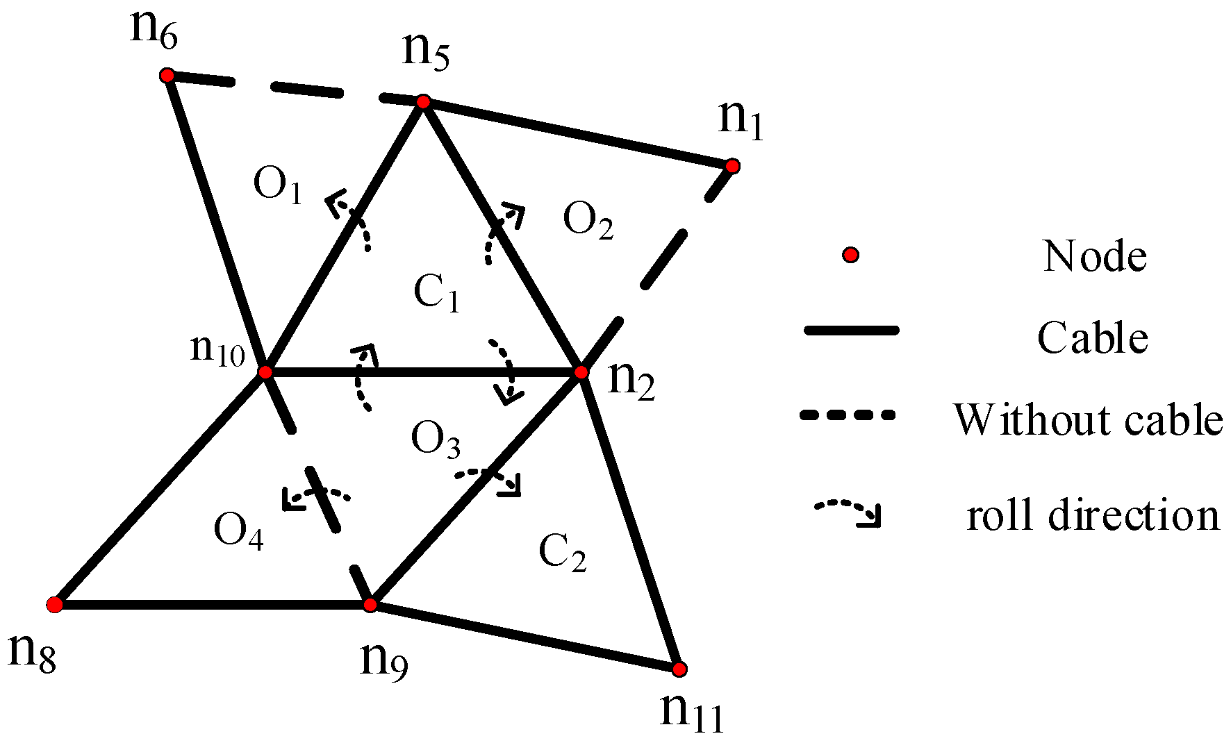
The motion gait planning of the closed triangle landing is shown in Figure 8. The robot can deform itself to offset the center of gravity. When the center of gravity crosses a line to reach another triangle, the robot rolls.

The center of gravity change of the CO-step was calculated through MATLAB software to verify the correctness of the rolling principle. As shown in Figure 9, the empty green circles, red stars, and thin dotted lines represent the node positions, the center of gravity, and the moving direction of the center of gravity, respectively. The red dotted line represents the tumbling edge. The change in the COC-step center of gravity is shown in Figure 10.

The gait planning of the six-bar tensegrity robot is the path planning of selecting the appropriate rolling gait many times according to the landing method, which finally reaches the target point. In addition, due to the large value of the gravitational moment of the OO-step, the robot rolls with difficulty; thus, the OO-step is not chosen in this paper during the rolling process.

4.3. Continuous Roll

Since the adjacent triangles of the closed triangle are all open triangles, which can better achieve locomotion, the closed triangle is chosen in this paper for continuous gait planning. Since the continuous roll is composed of multiple OC, CO, or COC steps, it will not be repeated in this section.

After analysis, the closed triangle can achieve the basic linear locomotion of the robot through six COC steps, as shown in Figure 11, and can also achieve the robot’s basic steering movement through four COC steps, as shown in Figure 12.

Based on this, a continuous locomotion calculation example is set up in this section from the initial state of a closed triangle landing locomotion to the end state of a closed triangle. As shown in Figure 13, the initial point is a red dot, and the end point is a blue dot. Different colored polylines represent different gaits.

4.4. Obstacle Avoidance Roll

In order to further verify the gait of the above analysis, locomotion experiments and a target points were set up. In order to verify the ability of the robot to move to any target, an obstacle was set at the line connecting the two dots. Figure 14 is the obstacle avoidance gait planning diagram. The initial point is the red dot; the end point is the yellow dot; the blue polyline is the imagined gait, and the brown strip is the set obstacle.

5. Prototype Development of the Six-Bar Tensegrity Robot

Based on the previous configuration design, the six-bar tensegrity robot prototype was developed to verify the rationality of the previous configuration. According to the gait planning, a prototype experiment was carried out, which provided the experimental basis for the follow-up kinematic analysis and trajectory planning.

5.1. Prototype Development of the Six-Bar Tensegrity Robot

In order to achieve the locomotion control of the robot, the control system of the six-bar tensegrity robot was designed. Among others, the main control chip uses the STM32F103C8T6 minimum system board, which has high adaptability, stable performance, and low power consumption; the motor drive module TB6612FNG can control two linear motors as the drive module; the MP1584EN chip is used as the power supply step-down voltage regulator module, and the HC-05 Bluetooth module is used as the signal input of the robot prototype controller. The controller of the robot prototype is shown in Figure 15.

According to the experiment, a miniature electric push rod is selected to simulate the rod member. The push rod has two control modes: a position-blocking switch and position-negative feedback adjustment. When the push rod reaches the limit position, the blocking switch is triggered, and the power supply is cut off. Through the negative feedback of the position, the telescopic part of the push rod can be controlled, and precise control of the push rod can be achieved. The maximum thrust of the electric push rod is 22 N, and the driving force provided by it can achieve the rolling of the robot.

The cable members in this prototype use Kevlar cables and cylindrical stainless-steel springs that vary with the length of the rod members. The use of rod and cable components meets the needs of the robot prototype.

In this section, the original length of the rod member of the robot prototype is 300 mm. According to the form-finding structure above, the length of the cable member and the rod spacing can be obtained to build the six-bar tensegrity robot prototype. In order to reduce the influence of uneven mass distribution at both ends of the linear push rod motor, each group of parallel linear push rod motors adopts positive and negative installations. In order to study the motion mode of the six-bar tensegrity robot and verify its movability, the prototype of the six-bar tensegrity robot is manufactured by electric actuators, Kevlar cables, and 3D-printed joints. The joint is designed as an arc-integrated shape that differs from the structural model, which plays a role in protecting the electric actuators and enhances its motion performance, as shown in Figure 16. The robot prototype basically maintains the shape of the six-bar tensegrity structure in a static state, and there is no obvious deformation. The basic parameters are shown in

Table 5. The basic parameters of the robot prototype.

Items	Value
Original length of electric push rod (mm)	300
Maximum length of electric push rod (mm)	350
Shortest length of electric push rod (mm)	200
Telescopic speed range (mm/s)	20
Rod Spacing (mm)	150
Cable length (mm)	183.7
Electric push rod mass (kg)	0.11
Battery mass (kg)	0.17
Controller mass (kg)	0.03
Total mass of robot prototype (kg)	1.27

.

5.2. Single-Step Roll Experiment

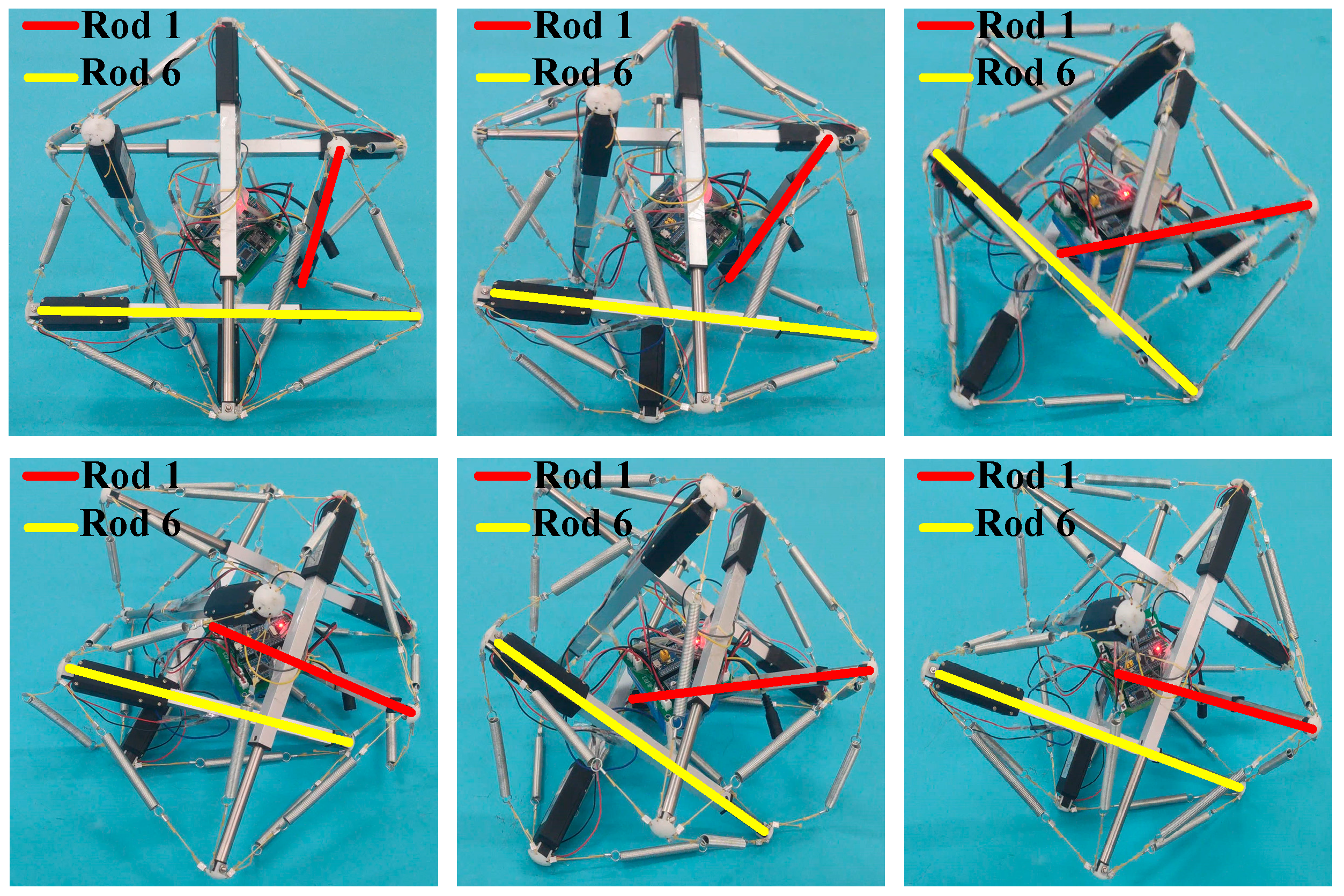
The robot prototype in Figure 16 is in an open triangle landing state. When the length of one or two rod members is controlled through Keil5 software programming, the single-step rolling locomotion of the CO- or OC-step of the six-bar tensegrity robot can be achieved. When the robot touches the ground in a closed triangle, Rod 2 and Rod 6 are shortened by 50 mm at the same time. At this time, the structure of the robot is seriously deformed. When the rod members of the original lengths are restored, the robot prototype becomes balanced, and the robot prototype achieves the rolling locomotion of the CO-step. The actual rolling process is shown in Figure 17. When the robot touches the ground in an open triangle, Rod 1 and Rod 6 are shortened by 30 mm at the same time. Then, the rod members are restored to their original lengths. Subsequently, the robot prototype achieves the rolling locomotion of the OC-step. The actual rolling process is shown in Figure 18.

5.3. Continuous Roll Experiment

Based on the single-step roll experiment, the experiment of continuous locomotion of the robot prototype is discussed in this section. According to the previous gait analysis, controlling different motors can make the robot accomplish continuous locomotion and verify the coordination and mobility of the robot.

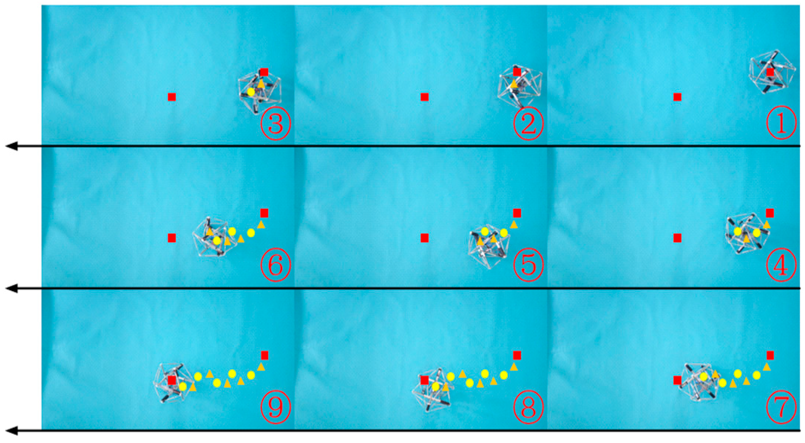
As shown in Figure 13, the red and blue lines only need to go through 11 COC steps to reach the designated position, which is shorter than those of other paths. In this paper, the blue path is selected for verification. The actual locomotion process is shown in Figure 19. In the figure, the red dots represent the starting point and the endpoint, the orange triangles represent the gravity center position of the closed triangles of the robot prototype, and the yellow circles represent the gravity center position of the open triangles of the robot prototype.

5.4. Obstacle Avoidance Roll Experiment

According to the above experimental contents, to further verify the robot locomotion performance, the robot is controlled to complete obstacle avoidance according to the gait planning in Figure 14, and the actual obstacle avoidance rolling locomotion process of the robot prototype is shown in Figure 20. Among them, the red dots represent the starting point and the endpoint, the orange triangles represent the gravity center position of the closed triangle of the robot prototype, the yellow circles represent the gravity center position of the open triangles of the robot prototype, and the wooden blocks represent obstacles or dangerous areas.

During the experiment, it was found that there is a difference between the actual locomotion gait and the planning gait. This difference may be caused by the quality and load of the robot itself. We tried to reduce the imbalance of the load on the robot structure and place the load on the robot centroid location as much as possible.

6. Conclusions

In this paper, by establishing an equilibrium matrix, the singular value decomposition method was used to obtain the configuration design of a six-bar tensegrity robot, which is also suitable for the form-finding of an asymmetric tensegrity structure. Based on the form-finding results, the six-bar tensegrity and the star tensegrity models were successfully built, all of which meet the definition of the tensegrity structure and verify the rationality of the form-finding method. According to the rolling principle of the six-bar tensegrity robot, the gait planning of the single-step, continuous, and obstacle-avoidance rolling of the robot was designed. The six-bar tensegrity robot prototype was developed, and the rolling and obstacle avoidance experiments were conducted, verifying that the robot has a strong locomotive performance. The experiments show that the uneven distribution of the robot’s mass and load causes accuracy errors regarding the motion. In-depth research on the new mass equilibrium configuration of the six-bar tensegrity robot and dynamics modeling that considers the influence of the relaxation and nonlinearity of the cables is planned for future work.