Fast Support Vector Machine for Power Quality Disturbance Classification

Abstract

The power quality disturbance (PQD) problem involves problems of voltage swell, voltage sag, power interruption, harmonics and complex events involving multiple PQD problems. The PQD problem attracted considerable attention from utilities, especially when renewable energy is getting a higher penetration. The PQD problem could downgrade the service quality, causing problems of malfunctions and instabilities. This paper proposed a simplified SVM technique to identify the PQD problem including the multiple PQD classification. With the simple structure proposed, the methodology could reduce a great deal of training data; requires much less memory space and saves computing time. An IEEE 14-bus power system was used to show the performance. Many tests were conducted, and the method was compared with an artificial neural network (ANN). Simulation results showed the shortened processing time and the effectiveness of the proposed approach.

1. Introduction

The PQD problem involves problems such as voltage swell, voltage sag, power interruption, harmonics and complex events involving multiple PQDs stated above [1,2,3,4]. Voltage swell and sag could occur from false VAR compensations, such as the starting of big motors, capacitor switching, short circuits, thundering or artificial calamity. Power interruption could be accompanied by voltage problems, and it will be defined by specific terms used in this paper. Harmonic currents are generally injected by the growing number of non-linear loads to degrade the quality of services, which are especially harmful to sensitive customers, such as the most recent 11 March 2022 blackout in Taiwan, causing a great deal of threat to the high-tech semiconductor scientific parks. Besides the above-mentioned PQD problems, the development of massive rapid transit system and high speed railway have also integrated advanced semi-conductor technologies in the auto-traction system, causing additional harmonics which are also considered in [3]. These electronic devices and non-linear loads further worsened the harmonic distortion problem. Now the PQD problem is not only important, but also accompanied by the problem of detecting the PQD location and types.

With the widespread power system, power engineers will be inundated with an enormous amount of data for inspection, as traditionally inspected visually, it requires the engineer’s critical knowledge. There are many papers published in this field [1,2,3,5,6,7,8,9,10,11,12,13]. Conventional methods involve techniques like FFT, and transformation algorithms by Hilber-Huang, Gaber, slant; improved chirplet, and so on [5,6,7,8]; a fast and reliable digital method for identifying and detecting various disturbances [9,10,11] is of a great value. DSP techniques, mathematical morphology-based methods were also used [12,13]. Besides conventional methods, artificial intelligence has also been developed and applied including GA, PSO, ACO, BCO, ANN and SVM for PQD classification [14,15,16,17,18,19].

Combining the conventional idea and AI, as a typical example in [4], Fast Fourier Transformation (FFT) and Artificial Neural Network (ANN) were integrated to solve the PQD problem. Note that the harmonic measurements are different from the ordinary power system measurements, where most harmonic measuring equipment were designed with FFT techniques and digital filtering, with a suitable bandwidth (3 kHz) for recording the waveforms. FFT is used to analyze distorted waves and filter out the fundamental waves to detect harmonic components. With FFT [3], the recorded waves were digitized and processed to extract the deformed waves; the Artificial Neural Network (ANN) then followed to detect the harmonics, as conducted in [4]. The FFT technique has limits with the number of samples, the memory and the processing time, while the ANN has difficulties in determining the number of hidden layers and nodes. Training an ANN is slow and time consuming, in the meantime, global optimum will not be guaranteed [3,20,21,22]. ANN accuracy requires more samples in determining the architectural design, where the time consuming process becomes another burden, regardless of the proposed idea of using the partial connecting ANN network [11].

Considering these limitations, a simplified form of the support vector machine (SVM) [23,24,25,26,27] is proposed in this paper for PQD. SVM is regarded as a better classifier than conventional methods for pattern recognition [28,29]. There are also some publications in the PQD field with SVM [30,31]. An SVM is a learning machine with interesting theoretical characteristics [23,24,25,26]. The so-called support vectors (SVs) could identify the decision boundaries of classes, which are near the separation surface of various classes, and it is a critical feature for correct classifications. SVM structure has renowned binary classification capability, which will be extended in this paper, for multi-class PQD problems. A simple linear SVM machine, nonlinearly related to the input space, allows fast training techniques, even with big training sets and a large number of input variables [25]. The simple binary classification SVM can be interpreted into the one-versus-one (OVO) structure [29] for a multi-class problem, called the Fast SVM (FSVM) in this paper. FSVM uses standard quadratic optimization. It is very fast and ensures global optimality, which is not easily attainable by other methods [20,21,22]. Many tests were conducted, and a sample IEEE 14 bus power network was provided to show the simulation results, and comparisons with other ANNs were provided to show the effectiveness

2. Fundamental Theory

An SVM, a learning paradigm proposed by Vapnik et al., is effective for both regression problems [24,25], and pattern recognition [25,26,29]. An SVM can deal with linear and non-linearly separable models from the statistical learning theory [23]. In addition, an SVM is a linear machine of one output, based on theoretical derivation, the number of hidden units is equal to the SVs, closest to the separation plane for different classes.

An SVM optimizes the tradeoff between the training errors and Vapnik–Chervonenkis (VC) dimension and provides a concept of complexity measure [24,25,26]. For complex data, the SVM is extended to work in the high dimensional space with nonlinear mapping from the K-dimensional input vector into R-dimensional feature space (R > K) through a kernel function. This structural risk minimization (SRM) framework generalizes the empirical risk minimization (ERM) principle applied for ANN training [25,26].

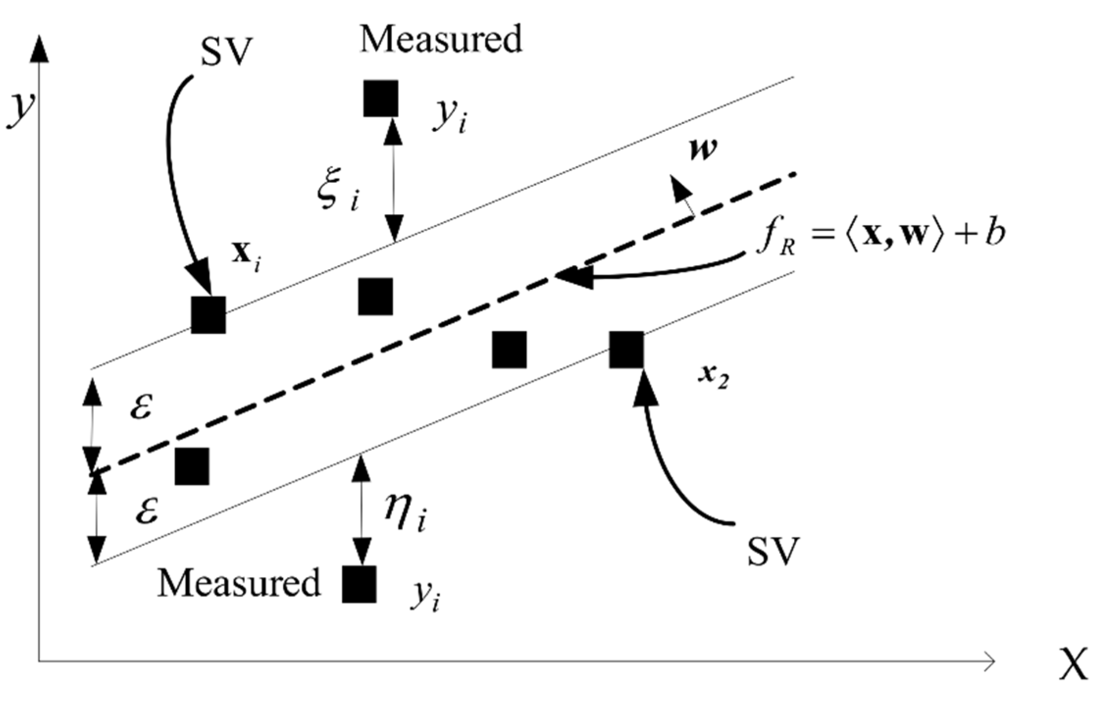
For the two-class problems, SVM is based on a hyper-plane to separate the data. Consider an n-dimensional real-valued input vector x_i, $x_i\in {\Re }^n$ of the training set $\mathrm{Tr}={\{(x_i,y_i)\}}_{i=1}^l$, where $y_i\in$ {−1, +1} is the classification that determines the class of x_i. The hyper-plane can be determined by w, an orthogonal vector, and a bias b satisfying w^Tx + b = 0, as shown in Figure 1. The classification becomes the problem of finding the hyper-plane to separate the classes, i.e., to maximize the distance between classes, called the ‘margin of separation M’. The hyper-plane can be found using the training sets, by the nearest points to it with the largest margin, i.e., the so-called SVs. The hyper-plane depends on the SVs. In a simple form, SVMs learn the linear decision rules by

$$f(x)=sign(w^{T}x+b)$$

(1)

so that (w, b) are needed to classify the training examples to maximize M.

To show the theory, consider that we can always scale w and b so that

$$w^{T}x+b=\pm 1$$

(2)

for the SVs as in Figure 1, and by the same time, it is clear that for non-SVs, we will have

$$w^{T}x+b>+1 \mathrm{or} w^{T}x+b<-1$$

(3)

Using the SVs x₁ and x₂, the margin M can be calculated as

$$\mathrm{M}=\frac{w^T}{\Vert w\Vert }(x_1-x_2)=\frac{2}{\Vert w\Vert }$$

(4)

Maximizing M is equivalent to the primal optimization problem of minimizing

$$2^{-1}{w}^{T}w$$

(5)

subject to

$$y_i\cdot \left[\langle w,x_i\rangle +b\right]\ge 1 i=1,\hspace{0.17em}2,\hspace{0.17em}\dots ,\hspace{0.17em}l$$

(6)

where $\langle w,x_i\rangle$ = $w^T{x}_i$ is an inner product.

Minimization of cost Function (5) with constrain (6) is a quadratic optimization problem, and a unique solution can be found using the Lagrange multiplier α, we have

$$L(w,b,\alpha )=2^{-1}{w}^{T}w-{\displaystyle \sum _{i=1}^l{\alpha }_i[y_i(w^T{x}_i+b)-1]}$$

$\alpha ={[{\alpha }_1,\hspace{0.17em}{\alpha }_2,\cdots ,\hspace{0.17em}{\alpha }_l]}^T$ is the vector of Lagrange multipliers. It is easier to solve the dual problem (7) with (8) instead of solving for (5) and (6), by maximizing

$$L_d(\alpha )={\displaystyle \sum _{i=1}^l{\alpha }_i-}{2}^{-1}{\displaystyle \sum _{i=1}^l{\displaystyle \sum _{j=1}^l}{\alpha }_i{\alpha }_j{y}_i{y}_j}\langle x_i,x_j\rangle$$

(7)

subject to

$${\displaystyle \sum _{i=1}^l{\alpha }_i{y}_i}=0 \mathrm{and} 0\le {\alpha }_i\le C; i=1,\hspace{0.17em}2,\hspace{0.17em}\dots ,\hspace{0.17em}l$$

(8)

where 〈xi, xj〉 is a scalar inner product. C is a preselected positive penalty factor, acting as a trade-off between the two terms. We have

$$L_d(\alpha )={\displaystyle \sum _{i=1}^l{\alpha }_i-}{2}^{-1}{\displaystyle \sum _{i=1}^l{\displaystyle \sum _{j=1}^l}{\alpha }_i{\alpha }_j{y}_i{y}_j}\langle x_i,x_j\rangle$$

(9)

If we can find αi* (i = 1, 2, …, q) for the problem, the SVs are then the training points with αi* > 0. We will have

$$w^{*}={\displaystyle \sum _{i=1}^l{\alpha }_i^{*}}{y}_i{x}_i={\displaystyle \sum _{i\in Psv}^{}{\alpha }_i^{*}}{y}_i{x}_i$$

(10)

Choose any l $\in$ SVs, so 0 < αi* < C, then the optimal b* can be found by using

$$b^{*}=y_k-\langle w^{*},x_k\rangle =y_k-\langle {\displaystyle \sum _{i\in P_{sv}}{\alpha }_i^{*}{y}_i{x}_i,x_k}\rangle =y_k-{\displaystyle \sum _{i\in P_{sv}}{\alpha }_i^{*}{y}_i}\langle x_i,x_k\rangle \hspace{0.17em}$$

We can find the discrimination function with the optimal b*, that is

$$g^{*}(x)={\displaystyle \sum _{i\in SV}{\alpha }_i^{*}}{y}_i\langle x_i,x\rangle +b^{*}$$

(11)

In non-linear input mapping cases, the kernel function K is used; typical ones are the radial basis function, polynomial or sigmoid function. The function K(xi, xj) can be used to replace 〈xi, xj〉 in (11).

For simple data without non-linear mapping of K(xi, xj), the simplest SVM learning decision rule is

$$f*(x)=sign\hspace{0.17em}\hspace{0.17em}(g*(x))=sign\hspace{0.17em}\hspace{0.17em}({\displaystyle \sum _{i\in SVs}{\alpha }_i^{*}}{y}_i\langle x_i,x\rangle +b*)$$

(12)

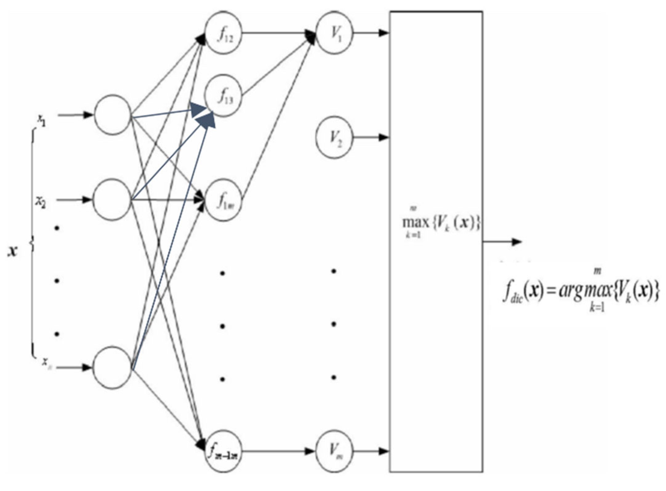
3. Design of the Fast SVM (FSVM)

The standard SVM used to solve the multi-class problems is in the form of one-versus-rest (OVR) approach [25], where the characteristics of one class can stand out against all the rest classes. The process may involve problems with complicated training data preparation. While basic SVM has renowned characteristics for binary classification, which we can utilize to improve the classification structure, such as the one-versus-one approach [25]. The size of the classification problem will be in proportion to the square of the number of classes, traded with the benefit of the simple decision rule of the separation plane. For classification problems with m classes, the design requires m(m − 1) /2 classifiers. The classifiers fij, 1 < i < j < m, needs training samples from class i and class j only, labeling the two classes by +1 and −1, respectively. This binary classification of the proposed FSVM needs no aids from any other complex techniques such as wavelet or FFT and is very fast. To extend the structure to m-classes, event i of FSVM has to win (or “stand out”) over all classes in each binary classification to distinguish event i from all other m-1 classes. In terms of the model, the number of “wins/scores” of FSVM is calculated by the frequency Vi of the test class xi. For xi, applying fij against all xj, where j ≠ i, the final decision is the most frequent class with the highest number of +1 counted, as shown in Figure 2, i.e.,

$$f\left(x\right)=\underset{ k=1}{argmax}{V}_k\left(x\right)$$

(13)

3.1. FSVM Classification System

Figure 2 shows the design architecture of the proposed FSVM. For a power system, Energy Management System (EMS) is generally implemented in the control center on top of SCADA, where the voltage and current are readily available. FSVM links to SCADA/EMS to get existing measurements, i.e., the voltages and currents. There are pre-selected observation locations with equipment installed to get measurements, namely Obs-1, Obs-2, …, Obs-q. Observation locations mean the buses of interests where harmonics exist. The bus voltage measurements received at a regular interval will be sent to a Data Processor for translation. The input signal of FSVMs is the amplitude of one cycle of the distorted wave. Receiving the distorted wave, each FSVM will perform pattern recognition to generate an output value. The fdis will output the decision according to the score of each class, the class with the highest score is the PQD. Some examples can be seen in [3,11] for disturbance classification including magnitudes.

3.2. Training Patterns Creation

In this paper, harmonics (harm) are defined as the situation where the branch currents and node voltages are polluted by the harmonic sources. Besides harmonics, we have the following PQD conditions as recommended in [32]:

PQD type	Voltage %	Duration
sag	10~90%	0.5 cycle~secs
swell	>110%	0.5 cycle~1 min
harm + sag	10~90%	0.5 cycle~secs
harm + swell	>110%	0.5 cycle~1 min
normal	95~105%	~
interruption	severe sag/blackout	<1 min

With the PQD defined, harmonic power flow [33] was used to create training patterns for FSVM and checked with [34]. Running the power flow, regular power models were used including

• transmission line model: pi-equivalent model,
• transformers: simplified R + jX,
• shunt magnetizing components: ignored,
• capacitors: capacitances varied with frequencies,
• generators: sub-transient model with reactance,
• linear loads: series impedances R + jX,
• nonlinear loads: harmonic current sources from field data.

The procedure of running the harmonic power flow is

• read system data,
• execute power flow with fundamental data,
• obtain fundamental voltages and harmonics,
• change linear loads into impedance,
• find equivalent current injection from non-linear load,
• change system components into equivalent circuit model,
• build Yh Matrix, with harmonic order h = 2, 3, 5, 7, 9…50,
• for an h, calculate harmonic voltages Vh = (Yh)⁻¹ ×I,
• if h < 50 go to 6,
• calculate total voltage distortion Vtd%,
• end.

4. Configuration of Test Example

Figure 3 shows an IEEE 14-bus system, with 15 lines, 5 transformers, 5 generator buses and non-linear devices as in

Table 1. Non-linear devices of 14-bus system.

Bus No.	Non-Linear Load	Main Harmonic Order
7, 11, 13	6-pulse rectifier	5, 7, 11, 13, 17, 19
4, 6	12-pulse rectifier	5, 7, 11, 13, 23
9	SFC	5, 7, 11, 13, 17, 19, 23
10	TCR	3, 5, 7, 9, 11, 13
12	DC Motor	5, 7, 11, 13, 17, 23

SFC: Static frequency converter; TCR: Thyristor-controlled reactor.

. There are in total eight observation locations in Area 1 and Area 2. The bus and line data of IEEE14-bus are from [3]. This is a balanced 3-phase network with devices in a single line diagram.

Harmonics were provided in constant current modes, with current sources from field data for harmonic orders used in [3], where the voltage distortion could also affect the neighboring buses, including various harmonic load combinations considered. Running harmonic power flow, we can simulate harmonic voltages at observation locations. As an example at Obs-4, training data collected systematically from the field can be used to create the associated input and output patterns. The disturbing events used for training FSVM at Obs-4 are shown in

Table 2. Disturbing events for training at Obs-4.

Voltage Disturbances

Voltage sag

Voltage swell

Voltage interruption

Voltage normal

Combination of Harmonic Sources

1 bus: {Bus4}

2 bus: {Bus4, Bus7}{Bus4, Bus9}{Bus4, Bus10}

3 bus: {Bus4, Bus7, Bus9}{Bus4, Bus7, Busl0}

{Bus4,Bus9,Bus 10}

Complex Disturbances

harmonics with voltage sag

harmonics with voltage swell

.

4.1. Sampling Type and PQD Code

Sampling points are taken by the amplitude of one distorted voltage cycle for each input. In this paper, there are five types of sampling rates with different numbers of samples considered for one wave cycle as in

Table 3. Types of sampling rate.

Type	No. Samples	Rate (kHz)
S1	16	0.96
S2	32	1.92
S3	64	3.84
S4	128	7.68
S5	60	3.6

.

FSVM is fed by possible PQD events as input patterns in real-time, and output will identify the class of the PQD event. Integer numbers from “1” to “7” were used for the codes of output patterns. There are seven events for each observation location, as shown in

Table 4. PQD codes.

Class	Symbol	PQD	Code
1	v1	sag	1
2	v2	swell	2
3	v3	harm	3
4	v4	harm + sag	4
5	v5	harm + swell	5
6	v6	normal	6
7	v7	interruption	7

and Figure 2.

4.2. Training Data Creation

More training data sets improve accuracy with the cost of training time. This research showed the efficiency of a minimal 55 data sets. Representative sampling points is another key for effective classification. There are 55 sets of training data created for the FSVM at each observing location with sampling rates S1–S4 corresponding to the node number of input xi in Figure 2. The number of training sets for each disturbing event is

Class	PQD	voltage	no. training sets (55)
1	sag	−(10–30%)	11
2	swell	+(10–30%)	11
3	harm	load combination	7
4	harm + sag	class (1 + 3)	11
5	harm + swell	class (2 + 3)	11
6	normal	±5%	2
7	interruption	−90%	2

4.3. Design Architecture of the Test System

In this study, a preselected penalty factor C = 50 is used for expression (8). The Gaussian Radial Basis Function (GRBF) kernel is given by

$$\mathrm{K}\left(x,z\right)=\exp \frac{-{\left|\left|\mathrm{x}-\mathrm{z}\right|\right|}^2}{2{\rho }^2}$$

where the smoothing factor ρ=0.8 is used.

Table 5. Architecture of the FSVM.

Sampling Type	Network Size				Smooth Factor ρ
	I	H	V(i)	O
S1	16	21	7	1	0.8
S2	32	21	7	1	0.8
S3	64	21	7	1	0.8
S4	128	21	7	1	0.8

shows the architecture of the proposed FSVM developed by the authors, where the input, hidden, output nodes are shown. V(i)s are also hidden nodes.

For comparison purposes, a back-propagation neural network (BPNN) consisting of three layers was designed. There are the same 55 sets of training data used for BPNN.

Table 6. Architecture of the BPNN.

Sampling Type	Network Size			Learning Rate
	I	H	O	(L)_
S1	16	11	7	0.1
S2	32	15	7	0.1
S3	64	21	7	0.2
S4	128	30	7	0.2

shows the architecture of BPNN, designed and tested by authors in [3,20]. The conventional back-propagation learning algorithm is used for BPNN training [35].

BPNN and FSVM were both designed with an input number of nodes the same as the sampling points. One hidden layer for BPNN is used, and the experience formulas in [36] are used to determine the number of nodes in the hidden layer. As a general practice, parameters of both the FSVM and BPNN were acquired from the trial-and-error process. Many tests were conducted, and a few examples are shown for demonstration.

5. Simulation Results

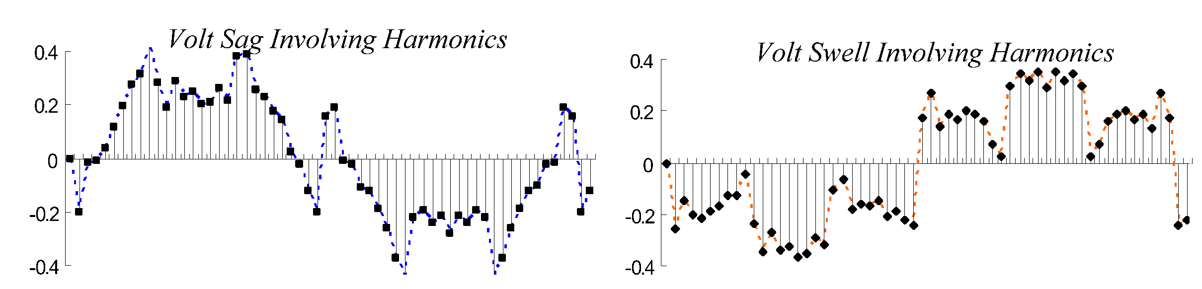
Running harmonic power flow, Figure 4 is a figure of type S5 in Table 3, with sampling rate 3.6 kHz and 60 samples. In this figure, the distorted wave was further processed by the discrete wavelet transformation (DWT) to show the pattern of harmonics in per unit. Besides this sample, neither DWT nor FFT were used in the proposed method.

Many tests were conducted, and the results at Obs-12 were shown for example with cross analysis to check the consistency and robustness. FSVM used type S2 in Table 3 with the sampling rate 1.92 kHz and 32 samples.

5.1. Voltage Change Detection with Cross Analysis at Obs-12

In this test, voltage magnitudes varied from 0% to 150% with the fundamental data at Obs-12, with an increment of 2% and 76 tests, i.e., 0~1.5 p.u. Various PQDs were identified according to the severity of voltage changes in each column, indicating the PQD values. For example, the first column shows the score of each PQD when the voltage is between 0~0.4. We can see the score in the order of v7 > v1 > v4 > v6 > v3 > v2. That is, it clearly identifies v7, the “interruption” as the PQD, followed by v1, the “sag” event. A cross check for v1 shows that the highest score takes place when the voltage (v) is above 0.42, i.e., 0.42 < v < 0.96. The v1 score drops onward as voltage rises above 0.96, i.e., v > 0.96. The v1, v2, and v6, other PQD events, get the highest score at various voltage magnitudes, while v3, v4 and v5 involving harmonics get low scores in all ranges in this test.

Table 7. Scores of each class for voltage variation at Obs-12.

PQD	0~0.4	0.42	0.6	0.96~1.0	1.04	1.06	1.1	1.3~1.5
v7	6	5	1	0	0	0	0	0
v1	5	6	6	5	3	3	2	2
v4	4	4	4	2	1	1	1	1
v6	3	3	5	6	6	5	5	4
v3	2	2	3	4	4	4	4	3
v2	1	1	2	3	5	6	6	6
v5	0	0	0	1	2	2	3	5

provides the cross-analysis information for voltage variations.

5.2. Harmonic Variations Detection with Cross Analysis at Obs-12

Detection accuracy is checked for harmonic PQDs in this test, where the harmonic injections varied 0~160% in magnitude, with an increment of 10% and in a total of 17 tests. In the first column, PQD points to v6 “normal” when there are no or very low harmonics, i.e., with harmonic magnitudes <0.3. We can see that v3, score of the harmonics gets higher when the magnitude is greater than 0.4, and stays highest onward. The complex event v4 and v5 get low scores, involving both harmonics and voltage changes. Other PQD terms also get low scores.

Table 8. Scores of harmonic variations.

PQD	0	0.1~0.3	0.4	0.6	0.8~1.0	1.2~1.6
v6	6	6	5	5	3	3
v1	5	3	3	1	1	1
v3	4	5	6	6	6	6
v2	3	4	4	2	2	2
v4	2	2	2	4	5	4
v5	1	1	1	3	4	5
v7	0	0	0	0	0	0

shows the scores of each class for harmonic magnitude changes. We can also see that v7 stays lowest through all tests.

5.3. Complex Disturbances Detection with Cross Analysis at Obs-12

Tests were conducted for complex events involving both harmonics and voltage disturbances. The harmonic injection stays the same while voltage magnitudes varied from 0~150% as in 5.2., with an increment of 2% and 76 tests.

Table 9. Scores of complex disturbances.

PQD	0~0.1	0.3~.036	0.38	0.6	0.92	0.94	1.06	1.08~1.1	1.3~1.5
v7	6	6	5	0	0	0	0	0	0
v4	5	5	6	6	6	5	3	3	2
v1	4	4	4	5	4	2	1	1	1
v6	3	2	2	4	2	3	2	2	3
v3	2	3	3	3	5	6	6	5	4
v5	1	1	1	2	3	4	5	6	6
v2	0	0	0	1	1	1	4	4	5

shows the scores for each class.

For harmonics with a voltage magnitude lower than 0.36, the PQD was identified as “interruption”. In the range 0.38–0.92, v4 was identified as “harmonics with sag”. For voltage magnitude 0.94~1.06, v3 “harmonic” was detected. For harmonics with a voltage magnitude >1.06, v5 was detected as “harmonic with swell”.

5.4. Multiple Harmonic Sources Detection

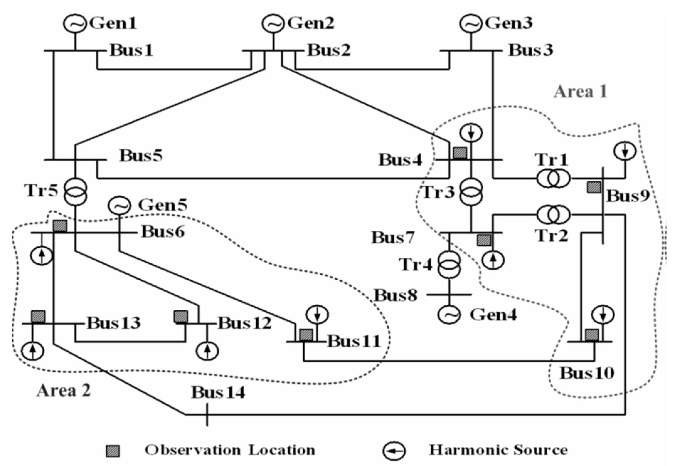
Sample S1 with 96 kHz and 16 number samples was used to show multiple harmonics detections in this test. Multiple harmonic sources were injected in both areas in Figure 3: Obs-4 and Obs-9 in Area1; Obs-11 and Obs-12 in Area2. Twelve distorted wave cycles were sampled for the time-domain analysis and fed to FSVM at each observation location.

Table 10. Scores of detections for multiple harmonics.

Loc	v1	v2	v3	v4	v5	v6	v7	fdis(X)
Obs-4	2	1	6	4	3	5	0	3
Obs-9	1	2	6	5	4	3	0	3
Obs-11	2	1	6	5	4	3	0	3
Obs-12	1	2	6	4	3	5	0	3

shows the detection result and the PQD. The mutually affected harmonics did not affect the results. All locations have fdis “3”, the highest value v3 being identified as “harmonics”. This example shows that FSVM is accurate enough with the lowest sample rates of 16.

5.5. Performances Test

Performance of FSVM and BPNN at Obs-4 for sampling Type S2 were compared in

Table 11. Performances test.

Method	C	L	Training Epochs	Training Time	Testing Time
FSVM	50	------	-----	1	1
BPNN	-----	0.1	40,000	220	1

. All weights were frozen for tests when the training finished. The training time of FSVM substantially outperformed BPNN, while the testing time is compatible. FSVM has a fast learning process without needing estimation for the hidden layer and the number of nodes. For comparison purposes, the training and testing times of FSVM was set to “1” as the base.

5.6. Detection Accuracy Test

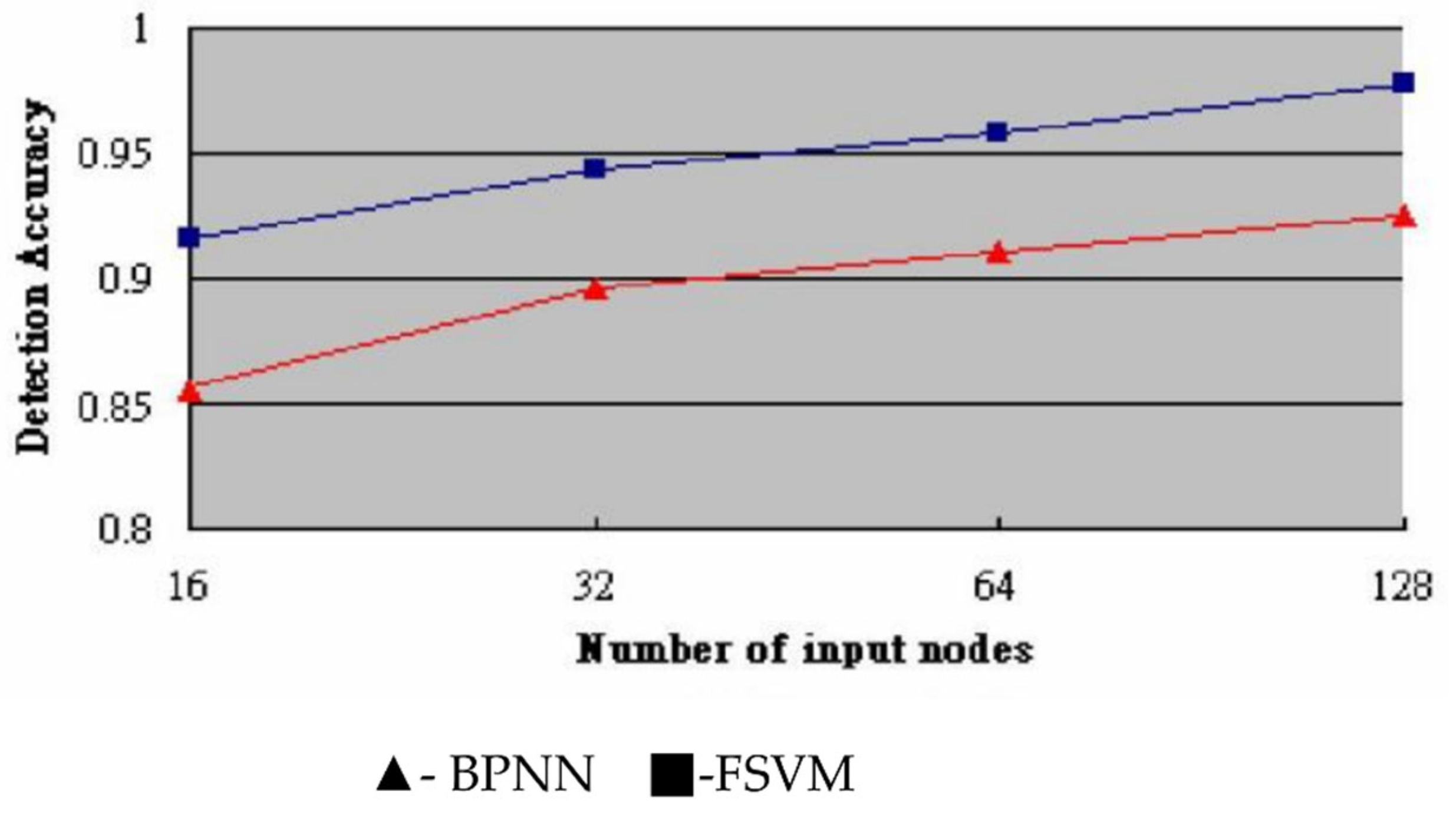
With 360 sets of random data for tests, the average accuracy for detection versus number of the input nodes at at Obs-4 can be seen in Figure 5. Both methods have higher accuracies as the number of sampling points increases. More training data could also improve the accuracy. This research showed examples of FSVM using 55 data sets and 16 nodes, where accuracy is greater than 90%, close to the 128-node BPNN without losing originalities of the wave distortion. Reducing the dimension from 128 to 16, we save a lot of data storage.

6. Conclusions

A classification technique FSVM for PQD problem was developed in this paper. FSVM based upon the binary classification, uses standard quadratic optimization. It is very fast and ensures global optimality, which is not easily attainable by other methods [20,21,22].

For m classes, a minimum sized network can be built with fast training, needing m (m − 1)/2 classifiers. It can extend to problems with more classes. Since the size is in proportion to the square number of classes, it is suitable for problems with limited classes such as PQD. The performance can be guaranteed by simplified structure, with less overhead and no ad hoc process like digital filtering, wavelet or FFT. The only required voltage information is already available in the control center. It is convenient to integrate FSVMs in a control center for PQD detection. The advantages of FSVM are summarized as

-

detects without needing extra measurement devices;

-

no need of digital filtering or FFT techniques;

-

a standard quadratic optimization problem, suitable for machine learning;

-

a simple learning algorithm to develop the hyper plane for classification;

-

training is very fast as compared to popular BPNNs;

-

a minimum sized network can be built with sufficient accuracy;

-

data storage reduces substantially with reduced dimension without losing the originality;

-

can detect complex events involving multiple harmonics and voltage disturbances.

FSVM trains the SVs, mapping to a higher dimension by using a kernel function, forming a standard quadratic optimization problem with a unique global optimum, which is a superior characteristic in dealing with non-linear problems.