An Improved Particle-Swarm-Optimization Algorithm for a Prediction Model of Steel Slab Temperature

Abstract

Aiming at the problem of the low accuracy of temperature prediction, a mathematical model for predicting the temperature of a steel billet is developed. For the process of temperature prediction, an improved particle-swarm-optimization algorithm (called XPSO) is developed. XPSO was designed based on a multiple swarm scheme to improve the global search capability and robustness; thus, it can improve the low accuracy of prediction and overcome the problem of easy entrapment into local optima. In the XPSO, the multiple swarm scheme comprises four modified components: (1) the strategy of improving the positional initialization; (2) the mutation strategy for particle swarms; (3) the adjustment strategy of inertia weights; (4) the strategy of jumping out local optima. Based on widely used unimodal, multimodal and composite benchmark functions, the effectiveness of the XPSO algorithm was verified by comparing it with some popular variant PSO algorithms (PSO, IPSO, IPSO2, HPSO, CPSO). Then, the XPSO was applied to predict the temperatures of steel billets based on simulation data sets and measured data sets. Finally, the obtained results show that the XPSO is more accurate than other PSO algorithms and other optimization approaches (WOA, IA, GWO, DE, ABC) for temperature prediction of steel billets.

1. Introduction

In the steel industry, the reheating furnace must reheat the material (slabs) to the desired uniformity temperature profiles at the exit. However, the slab reheating furnace’s operation is a complex physical and chemical process [1]. To better control and optimize the furnace’s operations, there should be a suitable temperature prediction model to predict the accurate temperatures for the slabs inside the furnace. Given the continuous development of artificial intelligence techniques, the demand for a suitable temperature prediction model is increasing [2]. Therefore, a suitable mathematical model which can predict the discharge temperatures of billets accurately and quickly should be proposed for the control and optimization of the reheating furnaces. In general, the prediction models can be divided into two categories [3]: the mechanism models based on first principles [4] and the empirical models based on the production data and black-box approaches [5]. The first kind of model needs to fully understand the physical and chemical processes inside the reheating furnace—e.g., [1,6,7,8]. The computational requirements of these models vary widely depending on the level of complexity [3]. Finally, the heat-transfer process is often summarized by partial differential equations (PDEs). Usually, mechanism models are complicated and nonlinear (such as those in ([9,10,11,12,13,14]). Hong et al. [13] investigated the sequential function specification coupled with the Broyden combined method (BC-SFSM) to obtain the temperature field of a steel billet based on the inverse heat-conduction problem. The results illustrate that the majority of relative errors during the whole reheating time are less than 5%. Chen et al. [14] presented a novel method to obtain these parameters by combining a "black box" test with a billet heat transfer model. The surface temperature and center temperature’s relative error were 2.34% and 3.51%, respectively. The numerical computation of PDEs will require a lot of computational time, which will exceed a practical time criterion. Therefore, this kind of model cannot satisfy the requirements for an online system.

The empirical models are often determined by identification methods involving the genetic algorithm (GA), support vector machines (SVMs), neural networks (NNs), particle swarm optimization (PSO) and other intelligent techniques ([15,16,17,18]). For instance, Thanawat et al. [19] investigated a prediction model using the production data from Ratchasima Steel Products Company. The GA method was used to identify the model’s unknown factors. Tang et al. [20] presented the SVM predictive model for the temperature control problem. The PSO was applied to determine proper parameters for the SVM model and finally obtained good performance. Wang et al. [21] constructed a prediction model of slab discharging temperature by combining GA with a BP neural network. The mean-square error of the network was 72.3477, and the error was lower than 20 °C. Yang et al. [22] used the relevance vector machine (RVM) method to predict the slab temperature. The maximum prediction error of slab temperature was 10.46 °C. In general, the empirical model is often simplified to a simple formula, so the calculation time is small enough to satisfy online production [23]. The production data and the performance of the intelligent algorithm used will determine the advantages and disadvantages of an empirical model. As the industrial software and database techniques continue developing, more production data are being obtained [24]. Thus, an intelligent algorithm with excellent performance is indispensable, and it behooves us to study the intelligent algorithms carefully.

The PSO algorithm has the characteristics of high solution accuracy and a fast approach to the optimal solution. However, the basic PSO varies in its ability to solve problems in different application contexts. It also easily falls into local optima. Researchers have studied various strategies for the improvement of PSO. For instance, Alsaidy et al. [25] proposed the longest job to fastest processor PSO (LJFP-PSO) algorithm and the minimum completion time PSO (MCT-PSO) algorithm for the task-scheduling problem. The effective performance of the two algorithms was proved by simulation results. Yue et al. [26] presented a novel multi-objective PSO that has ring topology for solving multimodal multi-objective optimization problems. The ring topology is used to form stable niches and locate multiple optima. Peng et al. [27] proposed a symbiotic PSO (SPSO) algorithm to control a water-bath-temperature system. A multiple swarm scheme was proposed for the SPSO algorithm. Three major components (create initial swarms, evaluating fitness values and updating each particle) are used to escape from a locally optimal solution.

Inspired by these algorithms, we propose an improved PSO (named XPSO) algorithm that uses the multiple swarm scheme in this paper. The scheme comprises four modified components: (1) improving the positional initialization of the particle swarms: one randomly generated and the other uniformly generated; (2) adding the mutation strategy for the particle swarm to increase its population diversity; (3) adjusting the inertia weight through a "stepped" adaptive model; (4) adding the strategy of escaping from the local minimized point.

This paper is presented as follows: the prediction model of the slab temperature is established in Section 2; the detailed strategies for improvement of XPSO are described in Section 3; the simulation and discussion are given in Section 4; Section 5 summarizes the conclusions.

2. The Prediction Model of the Slab Temperature

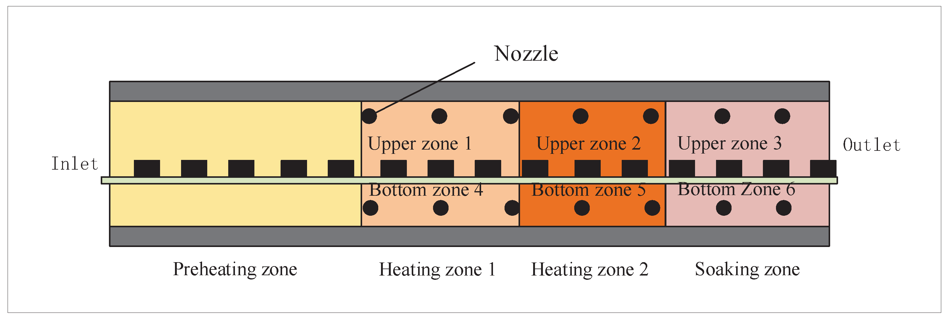
2.1. The Structure of a Reheating Furnace

The heat transfer processes in the furnace mainly consist of radiation heat transfer and convection heat exchange. The main function of reheating furnaces is to help the slabs reach the desired discharging temperatures for the next rolling process. The slab passes through the preheating zone, multistage heating zone and soaking zone from the furnace’s inlet to the outlet, as shown in Figure 1. The multi-stage heating zone can be divided into four subzones (upper zones 1 and 2; bottom zones 4 and 5), and the soaking zone is divided into two subzones (upper zone 3, bottom zone 6). The key components of a subzone are a series of regenerative burners, the corresponding furnace nozzle temperatures $T{N}_j$ and the furnace zone temperature $T{P}_k$. Here, $T{N}_j$ is easily obtained by the thermocouples nearby the location of burner’s nozzle j and $T{P}_k=\frac{1}{n}{\sum }_{j=1}^{n}T{N}_j$, which stands for the average value of the nozzle temperatures $T{N}_j$ in zone k.

2.2. The Prediction Model and Optimization Problem

The most important quality criterion of reheating furnace is the average outlet temperature of the steel slab. There are many factors affecting the slab’s discharging temperature. By analyzing the field data and some related research ([22,23]), we can confirm some key factors: the initial temperature of the billet, $T_0$; the furnace nozzle temperature, $T_j$; the mean temperature of each zone, $T_p$; the reheating time of the billet in the furnace, $\theta$; the material of the slab, $\alpha$; the thickness of the slab, d. Thus, the inputs of the prediction model are $X={[X_1,X_2,X_3]}^T$, which consist of the slab’s physical parameters, $X_1={[\alpha ,d,\theta ,T_0]}^T$; the vector of the furnace nozzle temperatures, $X_2={[T{N}_1,T{N}_2,\cdots ,T{N}_m]}^T$; and the vector of furnace zone temperatures, $X_3={[T{P}_1,T{P}_2,\cdots ,T{P}_6]}^T$. Notice, m is the total number of burners in the reheating furnace. The outputs are the predicted temperature $Y=TE$, which is the vector of the predicted temperatures of the slabs when discharged out from the furnace. Finally, the formula of predicting model is constructed as:

$$Y=f\left(X,W\right)=w_{0}d+w_1\alpha +w_2{T}_0^1+w_3{T}_0^2+\sum _{i=1}^{m}T{N}_i{w}_{\left(i+3\right)}T{N}_i+\sum _{j=1}^6{w}_{\left(j+m+3\right)}cos\left(T{P}_j\theta \right)+\sum _{j=1}^6{w}_{\left(j+m+9\right)}sin\left(T{P}_j\theta \right)$$

(1)

where $W=[w_0,w_1,\cdots ,w_{m+15}]$ represents the vector of unknown weight parameters, which will be determined by the proposed XPSO algorithm. The formula f is composed of a polynomial and a Fourier function, which was designed by the author based on experience. To make the analytical response Y equal to the measured value $Y^{*}$, an optimization problem should be established with the objective of minimizing the error between the theoretically calculated values and the measured data. To alleviate overfitting and improve generalization performance, the strategy of regularization is employed for the optimization problem. Finally, the formula of the optimization problem is shown as follows.

$$\begin{array}{c}MinimizeJ={\parallel Y-Y^{*}\parallel }^2+{\lambda }_1\parallel W\parallel +{\lambda }_2{\parallel W\parallel }^2\\ st.Y=f\left(X,W\right)\end{array}$$

(2)

where $Y^{*}$ represents the measured temperature of the slab, and ${\lambda }_1,{\lambda }_2$ are the regularization parameters.

3. Improved Particle-Swarm-Optimization Algorithm

3.1. The Basic PSO Algorithm

The PSO algorithm originates from a researcher observing the social behavior of a flock of birds or fish [28]. Each particle in the population is a potential solution to the objective function. The particle has two attributes: velocity $V_i=\left[v_{i1},v_{i2},\cdots ,v_{ij},\cdots ,v_{ND}\right]$ and position $X_i=[x_{i1},x_{i2},\cdots ,x_{ij},\cdots ,x_{ND}]$, where $i=1,2,\cdots ,N$—N is the size of particle swarm; and $j=1,2,\cdots ,D$—D is the dimension of the solution space.

In each iteration, the information of individual particle is filtered to find the information about the historically optimal position p of the individual and the historically optimal position g of the population. The known information is brought into the velocity updating equation, Equation (3), and the position updating equation, Equation (4), to adjust the search direction of the population, so that the particle swarm approaches the global optimal solution, which is the optimal position of the population.

$$v_{ij}\left(k+1\right)=w{v}_{ij}\left(k\right)+r_1{c}_1\left(p_i-x_{ij}\left(k\right)\right)+r_2{c}_2\left(g-x_{ij}\left(k\right)\right)$$

(3)

$$x_{ij}(k+1)=x_{ij}\left(k\right)+v_{ij}(k+1)$$

(4)

where w represents the inertia weight; $r_1,r_2\in [0,1]$ are two uniformly distributed random values; $c_1,c_2$ are the acceleration parameters, which are non-negative constants; k represents the current iteration; and $k=1,2,3,...,G$, where G is the maximum number of iterations. The velocity updating of the particle is influenced by three factors: the current moment particle velocity $V_{ij}\left(k\right)$, the particle’s self-experience $\Delta V_P$ and the experience of particle swarm $\Delta V_g$. $\Delta V_P$ is the part of the particle that learns from its historical information, and $\Delta V_g$ represents the part of the particle that learns from the historical information of other particles within the population.

3.2. Improvement Strategies of the XPSO Algorithm

The basic PSO algorithm is a non-globally-convergent optimization algorithm [29]. To reduce the premature probability of falling into a local optimal solution and improve the convergence speed of the basic PSO, an improved PSO (named XPSO) algorithm is proposed based on the multi-strategy co-evolutionary approach. Four specific improvements are described as follows.

• Improving the positional initialization of the particle swarm: one randomly generated and the other uniformly generated.
  In a basic PSO algorithm, all of the particles are randomly initialized. The expression is given as follows:

  $$X_{ND}=\left[\begin{array}{cccc}l{x}_{11}& x_{12}& \cdots & x_{1D}\\ x_{21}& x_{22}& \cdots & x_{2D}\\ ⋮& ⋮& \ddots & ⋮\\ x_{N1}& x_{N2}& \cdots & x_{ND}\end{array}\right]$$

  (5)
  An increase in the positional diversity of particle swarms can facilitate the exploration of global range. However, increasing the diversity of particle swarms also makes it difficult to converge to the global optimum every time. Hence, an improved approach, based on the “double-edged sword” nature of particle swarm’s diversity, is proposed to improve the algorithm’s stability. During the initialization of the particle swarm, a dimension called X-Dim in the position matrix is randomly selected. The positional information of the particle in X-Dim is generated according to a uniform distribution, as shown in Equation (6).

  $$x_{ij}=\frac{O_{max}-O_{min}}{N}\ast i$$

  (6)

  where j is the randomly selected dimension; and $O_{max}$ and $O_{min}$ are the upper and lower limits of the value range of independent variables in different dimensions, respectively.
• The mutation strategy is introduced into the position updating of particle swarm to compensate for the decline in the overall diversity of particle swarm after improved initialization.
  Unlike some other meta-heuristic algorithms, standard PSO has no evolution operators such as crossover or mutation. The mutation strategy will be implemented by screening the particles in each iteration. If the corresponding fitness function value of someone particle is lower than the average fitness function value, the mutation strategy is performed in the current iteration. The formula of positional mutation is:

  $$x_{ij}^{*}\left(k\right)=x_{ij}\left(k\right)-w{v}_{ij}\left(k\right)-w\left(g-p_i\right)$$

  (7)

  where $x^{*}$ denotes the position of the particle after mutation.
• The adjustment of inertia weight is given to improve the flexibility of particle flight speed change, and the idea of “stepped” adaptive change is injected into the updating of inertia weight.
  Inertia weight w is directly related to the convergence speed. Most researches use the subtraction function as its updating formula for inertia weight [30]. Some others use the “stepped” improvement method to update the inertia weight [31]. In our method, the inertia weight is adjusted by combining the strategy of decreasing function and the “stepped” improvement. The specific change is given as follows:
  • A “three-step” strategy is proposed to switch the range $[w_s,w_e]$ of inertia weight by determining the fitness function value of the best position so far. The switching formula is given as follows:

    $$\left[w_s,w_e\right]=\left\{\begin{array}{cc}\left[w_{s1},w_{e1}\right]\hfill & f\left(g\right)\gg Fitness1\hfill \\ \left[w_{s2},w_{e2}\right]\hfill & Fitness2<f\left(g\right)<Fitness1\hfill \\ \left[w_{s3},w_{e3}\right]\hfill & f\left(g\right)\ll Fitness2\hfill \end{array}\right.$$

    (8)

    where $[w_s,w_e]$ is the range of inertia weight; $f\left(g\right)$ is the fitness function value corresponding to the global optimal solution; $Fitness1$ and $Fitness2$ are the autonomous set values. The values of $(\left[w_{s1},w_{e2}\right],[w_{s2},w_{e2}]$ and $[w_{s3},w_{e3}])$ need to be adjusted according to the conditions of the objective function in different application contexts.
  • After the ranges of the inertia weight $[w_s,w_e]$ have been determined, a decreasing function is introduced to adjust the w. The switching condition is related to the fitness function value of the best position so far. The update formula is given as follows:

    $$w=\left\{\begin{array}{cc}\frac{r sin\left(w_s\pi \right)}{4},\hfill & f\left(g\right)\gg Fitness3\hfill \\ w_s-\left(w_s-w_e\right)\sqrt{\frac{K}{G}},\hfill & f\left(g\right)<Fitness3\hfill \end{array}\right.$$

    (9)

    where $r\in [0,4)$ is a uniformly distributed random number; and $w_s$ and $w_e$ are the initial and final values of the range $[w_s,w_e]$ of the inertia weight, respectively. $Fitness3$ is the autonomous set value, k is the current iteration and G is the maximum iterations.
• The strategy of jumping out local optimum is proposed.
  A slope parameter $tr$ is given to judge whether the particle swarm has fallen in the local optimum. Here, $tr$ is the count of the condition when $Slope$ is less than the value $\epsilon$ in five iterations. The slope is calculated as follows:

  $$Slope=\frac{\left(f_k\left(g\right)-f_{\left(k-5\right)}\left(g\right)\right)}{5}$$

  (10)
  If the value of $tr$ equals the value of s, which is an autonomous set value, the particle swarm is trapped in a local optimum. Then, the particle swarm will perform a “jumping out local optimum” operation, which is done to change its position. The specific formula of a particle jumping out of a local optimum is given as follows:

  $$x_{ij}\left(k\right)=x_{ij}\left(k\right)-r_1{c}_1\left(g-x_{ij}\left(k\right)\right)+r_2{c}_2\left(bad-x_{ij}\left(k\right)\right)$$

  (11)

  where $bad$ represents the information of the global worst position. The core of this strategy is that the particle swarm should be nearest to the global worst position while staying away from the local optimum.

Finally, the pseudo-code of the XPSO algorithm is demonstrated in Algorithm 1.

Algorithm 1: The pseudo-code of the XPSO algorithm
1:	Initialize the parameters: (N, G, D, $O_{max}$,$O_{min}$, $V_{max}$, $V_{min}$, t, s, $\epsilon$)
2:	Combine uniform and random distribution to initialize position matrix $X_{N\times D}$
3:	Generate the initial velocity $V_i$ of each particle randomly
4:	Evaluate the fitness value of each particle
5:	Set $p_i$ with a copy of $X_i$
6:	Initialize g and bad with the best and worst fitness value among population
7:	While$k<G$
8:	If $k\ge 6$
9:	Update the slope of the fitness function curve
10:	Slope = ($f{\left(g\right)}_k-f{\left(g\right)}_{k-5}$)/5
11:	If $Slope\le \epsilon$
12:	t = t + 1
13:	End If
14:	End If
15:	Update inertia weight $\omega$ by Equations (8) and (9)
16:	For $i=1:N$
17:	Update the velocity $V_i$
18:	$v_{ij}\left(k+1\right)=w{v}_{ij}\left(k\right)+r_1{c}_1\left(p_i-x_{ij}\left(k\right)\right)+r_2{c}_2\left(g-x_{ij}\left(k\right)\right)$
19:	Update the velocity $X_i$
20:	If $t=s$
21:	For $m=1:50$
22:	$x_{ij}\left(k\right)=x_{ij}\left(k\right)-r_1{c}_1\left(g-x_{ij}\left(k\right)\right)+r_2{c}_2\left(bad-x_{ij}\left(k\right)\right)$
23:	End For
24:	Else
25:	$x_{ij}(k+1)=x_{ij}\left(k\right)+v_{ij}(k+1)$
26:	End If
27:	Calculate the fitness values of the new particle $X_i$
28:	Execute position mutation
29:	$x_{ij}^{*}\left(k\right)=x_{ij}\left(k\right)-w{v}_{ij}\left(k\right)-w\left(g-p_i\right)$
30:	Calculate the fitness values of the new particle $X^{*}$
31:	If $X_i\mathbf{or}{X}^{*}\mathbf{is}\mathbf{better}\mathbf{than}{p}_i$
32:	Update $p_i$
33:	End If
34:	If $X_i\mathbf{or}{X}^{*}\mathbf{is}\mathbf{better}\mathbf{than}\mathbf{g}$
35:	Update g
36:	End If
37:	If $X_i\mathbf{or}{X}^{*}\mathbf{is}\mathbf{worse}\mathbf{than}bad$
38:	Update bad
39:	End If
40:	End For
41:	k = k + 1
42:	End While

4. Simulations and Discussion

To verify the performance of the XPSO algorithm, some simulations are designed to involve both the performance and application of the algorithm. To obtain an unbiased CPU time comparison, all simulations were programmed by MATLAB R2017b and implemented on a computer with an Intel i5-11400F GPU, 2.60 GHz, 16 GB RAM.

4.1. Validation of XPSO by Benchmark Test Functions

The XPSO algorithm is compared with some popular variant PSO algorithms (PSO [32], IPSO [33], IPSO2 [30], HPSO [34], CPSO [35]) on a series of widely used optimization benchmark functions. A set of benchmark functions were selected from papers ([36,37]).

The benchmark set consisted of three main groups of benchmark functions: 4 unimodal (UM) functions, 2 multimodal (MM) functions and 3 composition (CM) functions. The UM functions (f1–f4) with a unique global best can expose the intensification capacities of different algorithms. The MM functions (f5–f6) can expose the diversification of algorithms. The CM functions (f7–f9) were selected from the IEEE CEC 2005 competition [37], which are also utilized in many papers to test the performances (balancing the exploration and exploitation inclinations and escaping from local optima) of algorithms.

The mathematical formulation and characteristics of UM and MM functions are shown in

Table 1. Descriptions of unimodal and multimodal benchmark functions.

Function	Name	Function’s Expressions	Search Range	Global Opt. 1
f1	Sphere	$f_1={\sum }_{i=1}^n{x}_i^2$	${[-100,100]}^n$	0
f2	Schwefel’s 1.2	$f_2={\sum }_{i=1}^n{\sum }_{j=1}^i{x}_j^2$	${[-100,100]}^n$	0
f3	Schwefel’s 2.21	$f_3=max\left\{\left|x_i\right|,1\le i\le n\right\}$	${[-100,100]}^n$	0
f4	Quartic Noise	$f_4={\sum }_{i=1}^{n}i{x}_i^4+random\left[0.1\right)$	${[-1.28,1.28]}^n$	0
f5	Generalized Rastrigin	$f_5={\sum }_{i=1}^n\left[x_i^2-10cos\left(2\pi x_i\right)+10\right]$	${[-5.12,5.12]}^n$	0
f6	Generalized Penalized Function 2	$\begin{array}{c}{f}_6=0.1{sin}^2\left(3\pi x_1\right)+0.1{\sum }_{i=1}^n{\left(x_i-1\right)}^2\left[1+{sin}^2\left(3\pi x_i+1\right)\right]\\ +0.1{\left(x_n-1\right)}^2\left[1+{sin}^2\left(2\pi x_n\right)\right]+{\sum }_{i=1}^{n}u\left(x_i,5,100,4\right)\end{array}$	${[-50,50]}^n$	0

¹ Global Opt.: global optimal solution.

. Details of the CM functions are shown in

Table 2. Details of hybrid composition functions.

Function (CEC2005-ID)	Description	Properties	Range	Global Opt.
f7(C16)	Rotated Hybrid Composition Function	MM 1, R 2, NS 3, S 4	${[-5,5]}^n$	120
f8(C18)	Rotated Hybrid Composition Function	MM, R, NS, S	${[-5,5]}^n$	10
f9(C21)	Rotated Hybrid Composition Function	MM, R, NS, S	${[-5,5]}^n$	360

¹ MM: Multi-modal, ² R: Rotated, ³ NS: Non-Separable, ⁴ S: Scalable.

. The parameters of both the PSO algorithms and the optimization problem (2) were as follows. The specific parameter combinations for the inertia weight were $[w_{s1},w_{e1}]=[0.9,0.4]$, $[w_{s2},w_{e2}]=[0.65,0]$ and $[w_{s3},w_{e3}]=[0.55,0.05]$. The maximum and minimum velocities of the particle were $V_{max}=0.1$ and $V_{min}=-0.1$, respectively. In addition, the acceleration coefficients $c_1$ and $c_2$ were selected to be 2.5 and 1.5, respectively. The inertia weight of the HPSO varied randomly in the range (0, 1). The parameters related to jumping out of local optimal were $s=270$ and $\epsilon =0.001$. The values of the regularization parameters in the optimization problem were ${\lambda }_1=1.2,{\lambda }_2=1.0$.

The maximum number of iterations for all benchmark functions (f1–f9) was selected as 8000. The dimensions of these benchmark functions (f1–f9) were selected as 10, 30 and 50. Thus, the performances of the six variant PSO algorithms can be compared in different dimensions.

Each algorithm was run individually 10 times, and the average statistical error was calculated. The mean of objective values (Mean) and standard deviation of its solving error (S.D.) were chosen as the performance measures for each algorithm. The simulation results are shown in

Table 3. Results of benchmark functions (Dim = 10, 30, 50).

F 1	D 2	XPSO		CPSO		IPSO		IPSO2		PSO		HPSO
		Mean 3	S.D. 4	Mean	S.D.	Mean	S.D.	Mean	S.D.	Mean	S.D.	Mean	S.D.
f1	10	1.29 × 10−102	2.89 × 10−102	3.42 × 102	2.07 × 102	5.81 × 10−8	2.39 × 10−8	1.07 × 10−3	2.38 × 10−4	7.95 × 10−9	1.63 × 10−8	2.33 × 10−8	6.15 × 10−8
	30	6.41 × 10−57	1.92 × 10−56	4.40 × 102	2.25 × 102	4.15 × 10−6	1.22 × 10−6	0.31	0.41	7.51 × 10−6	4.04 × 10−6	4.22 × 10−7	2.57 × 10−7
	50	1.59 × 10−8	3.89 × 10−8	4.57 × 102	2.80 × 102	1.93 × 10−5	5.87 × 10−6	6.73	13.42	2.00 × 10−5	1.30 × 10−5	1.02 × 10−6	3.08 × 10−7
f2	10	1.06 × 10−77	1.50 × 10−77	1.06 × 103	8.87 × 102	5.93 × 10−7	3.33 × 10−7	2.95 × 102	3.70 × 102	4.08 × 10−7	4.74 × 10−7	1.35 × 10−8	1.71 × 10−8
	30	8.67 × 10−12	1.23 × 10−11	4.36 × 103	1.95 × 103	1.44 × 10−3	4.36 × 10−4	9.07 × 102	8.11 × 102	5.74 × 10−3	2.33 × 10−3	3.11 × 10−5	1.98 × 10−5
	50	1.36 × 10−5	1.35 × 10−2	7.74 × 103	6.45 × 103	1.88 × 10−2	3.33 × 10−3	1.25 × 103	2.74 × 103	2.49 × 10−2	9.20 × 10−3	1.91 × 10−4	8.34 × 10−5
f3	10	1.11 × 10−21	1.91 × 10−21	4.59	1.13	2.70 × 10−4	1.47 × 10−4	6.41 × 10−2	7.51 × 10−2	4.45 × 10−4	2.61 × 10−4	8.41 × 10−4	7.47 × 10−4
	30	1.03 × 10−19	1.79 × 10−19	6.15	1.65	9.01 × 10−3	2.77 × 10−3	0.71	0.16	3.03 × 10−2	1.62 × 10−2	1.96 × 10−2	1.99 × 10−2
	50	6.84 × 10−5	1.37 × 10−4	4.87	0.65	0.23	0.22	5.76	0.41	0.36	0.33	0.13	0.11
f4	10	0.24	0.16	0.43	0.26	0.44	0.26	0.46	0.32	0.61	0.24	0.5	0.29
	30	0.27	0.2	0.58	0.28	0.53	0.32	0.35	0.3	0.64	0.31	0.52	0.18
	50	0.35	0.24	0.65	0.3	0.54	0.31	0.38	0.23	0.53	0.23	0.58	0.3
f5	10	12.93	3.98	12.08	4.46	10.45	4.43	9.3	3.4	10.94	4.09	9.83	4.16
	30	18.05	4.16	48.43	17.81	26.96	6.91	24.81	6.5	27.16	9.67	28.56	6.13
	50	20.9	2.54	67.23	18.56	38.51	11.94	34.18	4.93	39.99	14.36	33.73	10.42
f6	10	1.45	0.94	9.41	4.09	2.13	1.37	2.62	2.47	2.81	3.26	1.48	1.46
	30	5.08	3.56	25.39	5.56	14.51	8.42	22.09	5.69	9.49	5.42	6.59	6.24
	50	9.83	6.98	37.21	7.54	24.36	9.83	31.42	8.14	14.71	8.78	9.29	8.89
f7	10	196.35	26.50	502.96	179.38	381.96	94.03	731.48	80.86	362.11	36.18	428.34	59.63
	30	542.93	46.56	867.86	204.51	584.27	122.68	1223.15	110.51	505.28	80.91	623.86	90.26
	50	563.92	97.82	937.18	241.44	593.34	132.26	1378.35	129.68	599.16	106.17	651.98	126.37
f8	10	1090.72	41.53	1364.68	23.43	1135.18	22.51	1492.86	39.30	1136.88	65.80	1098.15	59.30
	30	1147.03	123.61	1408.69	50.61	1182.64	70.86	1561.77	56.23	1194.76	120.68	1287.80	84.09
	50	1167.73	134.83	1486.24	56.47	1202.59	132.75	1620.53	70.99	1249.79	131.05	1464.34	151.77
f9	10	1066.48	28.84	1387.39	19.11	1120.63	38.33	1538.21	9.21	1286.09	23.52	1287.69	39.38
	30	1291.78	38.31	1440.31	31.75	1319.86	43.93	1604.27	41.32	1303.97	30.27	1309.14	52.25
	50	1316.15	54.37	1485.75	41.98	1338.22	68.71	1633.61	82.42	1326.48	43.43	1524.77	68.02

¹ F: Function, ² D: dimensional, ³ Mean: mean of objective values, ⁴ S.D.: standard deviation.

and Figure 2, Figure 3, Figure 4, Figure 5, Figure 6, Figure 7, Figure 8, Figure 9 and Figure 10. Table 3 shows best values in bold.

According to Table 3, the XPSO algorithm is superior to other PSO algorithms in terms of solution accuracy. Considering the UM benchmark functions, the results of (f1–f3) solved by XPSO are better than those of the other algorithms. For f4, the best value of Mean was obtained by the XPSO algorithm for the (10, 30, 50)-dimensional cases. The best values of S.D for the (10, 30, 50)-dimensional cases were obtained by XPSO, HPSO and IPSO2. Except f5 in the 10-dimensional case and f6 in the 50-dimensional case, the results for the MM benchmark functions by XPSO are superior to those of the other algorithms. Based on values of the Mean of hybrid CM functions (f7–f9) in Table 3, high-quality solutions can be obtained by the XPSO algorithm.

The convergence curves of the mean of best function were plotted in Figure 2, Figure 3, Figure 4, Figure 5, Figure 6, Figure 7, Figure 8, Figure 9 and Figure 10 to enable clearer visualization of each algorithm’s performance. In Figure 2, Figure 3, Figure 4, Figure 5, Figure 6, Figure 7, Figure 8, Figure 9 and Figure 10, the XPSO algorithm does not show outstanding performance in the early stage of the solution, but its search capability is better in the late stage of the solution, and it can significantly improve the convergence speed in the late evolution. The reason is that the updating strategy of inertia weight includes the formula based on chaotic mapping; consequently, the global search has a high convergence speed for particles. In addition, the updating formula for inertia weight switched in local search, which resulted a slow flying speed of particles but improved the accuracy of the solution. Finally, it can be concluded that the XPSO algorithm has excellent performance in numerical optimization problems and can be used to solve problems in various application contexts.

4.2. Validation of XPSO by Benchmark Test Functions

Firstly, 1280 simulation data sets were generated based on the existing mechanism model to verify the validity of the XPSO algorithm. In total, 1200 data sets were randomly selected as training sets and the remaining 80 as test sets. Here, the XPSO algorithm is compared with not only other PSO algorithms (PSO [32], IPSO [33], IPSO2 [30], HPSO [34], CPSO [35]), but also the other optimization algorithms (WOA [38], IA [39], GWO [40], DE [41], ABC [42]). Secondly, the actual data sets were collected from a reheating furnace in Angang’s building. Fourty-three sets were randomly selected as the training sets. The remaining 10 sets were used as the test sets.

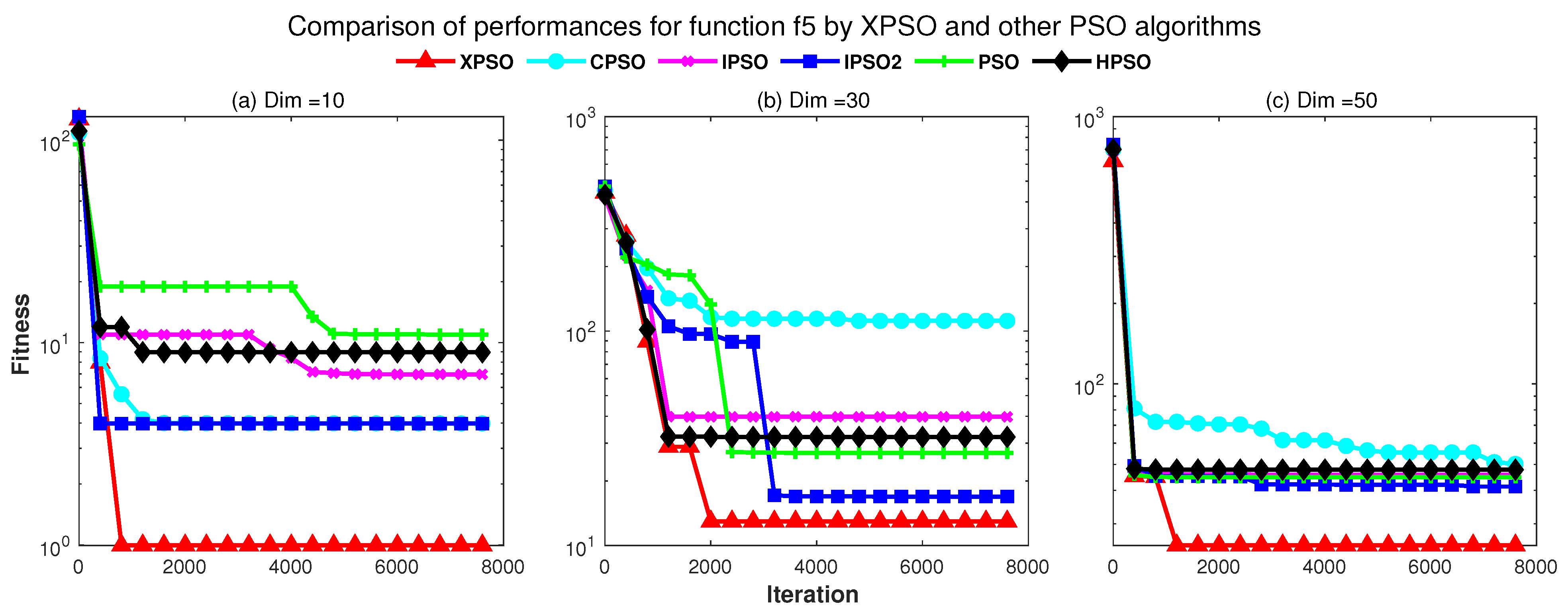
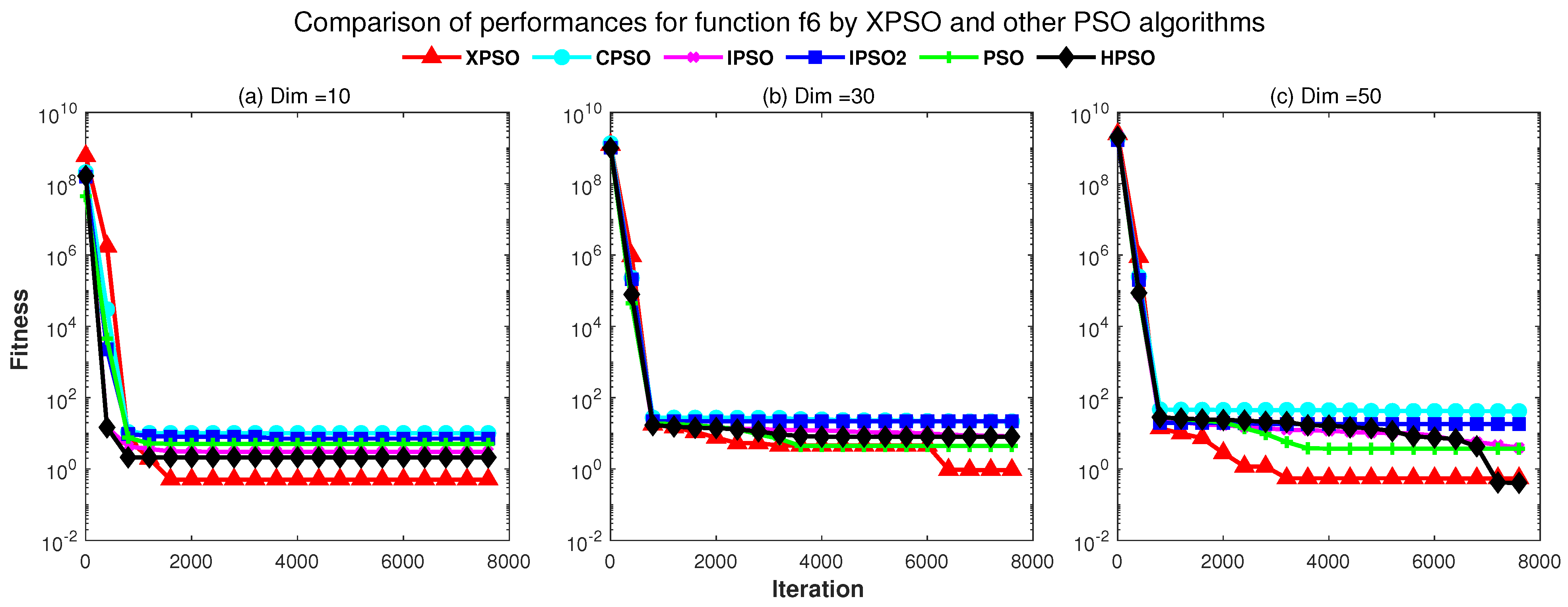
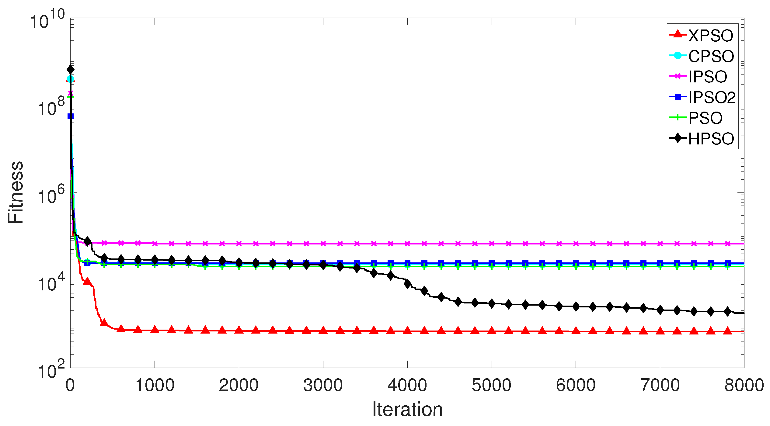
4.2.1. Comparison of XPSO and Other PSO Algorithms

Due to the random initialization of the PSO algorithms, each PSO algorithm independently ran 10 times. The relevant parameters for the PSO algorithms are shown in

Table 4. Classical benchmark functions.

Symbol	Name	Size
N	Particle swarm size	125
D	Particle Swarm Dimension	35
G	Maximum number of iterations	8000
$w_s$	Initial value of inertia weights	0.8
$w_e$	Final value of inertia weights	0.05
$c_1$	Acceleration coefficient 1	2.5
$c_2$	Acceleration coefficient 2	1.5
$V_{max}$	Value of maximum particle’s velocity	0.1
$V_{min}$	Value of minimum particle’s velocity	−0.1

. Each algorithm was evaluated by the mean, maximum, median, variance and standard deviation of the errors. The simulation results are shown in

Table 5. Classical benchmark functions.

Algorithm	Mean	Maximum	Median	Variance	S.D.
XPSO	0.55	2.29	0.46	0.216	0.465
CPSO	3.9	13.99	3.41	8.098	2.846
IPSO	7	23.75	5.85	26.582	5.156
IPSO2	3.76	13.58	3	8.388	2.896
PSO	3.58	11.65	2.77	6.818	2.611
HPSO	0.78	2.94	0.61	0.446	0.668

and Figure 11 and Figure 12.

In Figure 11, the XPSO algorithm clearly has a faster search speed than other algorithms in the early iterations and can quickly move to convergence. Table 5 shows that XPSO is also more accurate in terms of computational accuracy at the later stages of the iterations. Figure 12 ensures the accuracy of the proposed XPSO method for temperature prediction. The IPSO algorithm gave the worst results, for which the maximum error value was almost 24 °C. The mean and median prediction errors by the XPSO algorithm were 0.55 and 0.46 °C, and 99% of the prediction errors by the XPSO algorithm were within 2 °C.

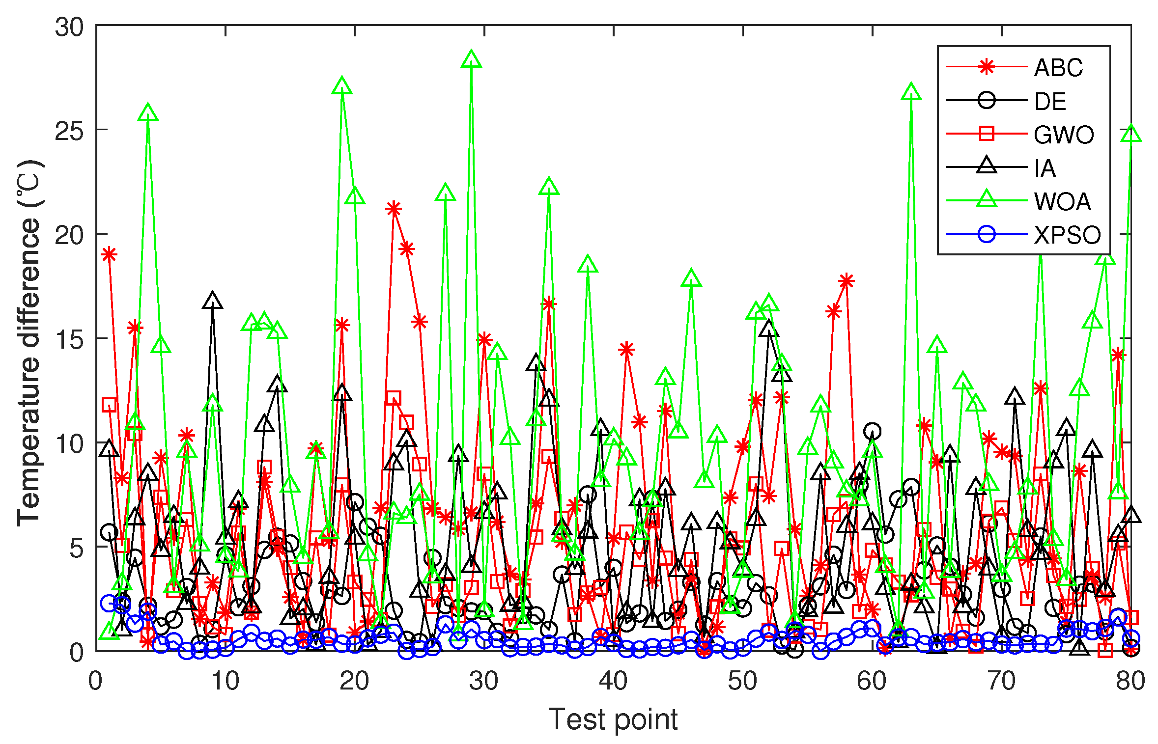
4.2.2. Comparison of XPSO and Other Optimization Algorithms

In this section, the XPSO algorithm is compared with the other optimization algorithms (WOA [38], IA [39], GWO [40], DE [41], ABC [42]) that have been proposed in recent years. The parameters of these algorithms are listed in

Table 6. Parameters of other optimization algorithms.

Algorithms	Population	Maximum Iteration	Dim	Other
WOA	125	8000	35	$r_1,r_2\in [0,1]$ are random numbers
IA	125	8000	35	$p_m=0.7,\alpha =\beta =1,\delta =0.2,ncl=10$
GWO	125	8000	35	$r_1,r_2\in [0,1]$ are random numbers
DE	125	8000	35	$F0=0.4,CR=0.1$
ABC	125	8000	35	$\alpha =1$

. Each algorithm was tested 10 times independently to reduce statistical errors. The mean, maximum, median, variance and standard difference of simulation results were recorded and are shown in

Table 7. Results of XPSO and other optimization algorithms.

Algorithm	Mean	Maximum	Median	Variance	S.D.
XPSO	0.55	2.29	0.46	0.216	0.465
WOA	4.53	28.27	3.45	18.94	4.3519
IA	6.92	27.52	6.43	28.0032	5.2918
GWO	2.28	13.39	1.2	6.6249	2.5739
DE	2.3	10.53	2.1	2.8971	1.7021
ABC	6.59	27.23	9.79	24.2055	4.9199

. The best results are shown in bold type. The convergence graph of each algorithm is shown in Figure 13. The slab temperature prediction errors of the XPSO algorithm and other optimization algorithms are shown in Figure 14.

Table 7 proves that the solution of the XPSO algorithm gives the best value. In Figure 13, the XPSO algorithm is more successful than all of the other optimization approaches, and the algorithm determined the global optimal solution after approximately 500 generations. As shown in Figure 14, the temperature prediction errors by the XPSO algorithm were much lower than the errors by the other optimization algorithms. The WOA algorithm gave the worst results; its maximum error value was almost 29 °C. In summary, the proposed XPSO algorithm exhibited fast search performance and accuracy when predicting the billet temperature based on simulation data sets. The results and figures show that this prediction model of billet temperature is credible and reliable. Its accurate prediction is expected to satisfy the future control needs of industrial reheating furnace systems, which will let operators adjust production plans in time to ensure efficiency and reliability.

4.2.3. Validation of the Temperature Prediction Model with Measured Data

The proposed XPSO algorithm was applied to predict slabs’ discharging temperatures based on actual data sets from Angang (company). The algorithm was independently run 20 times, and then the average prediction error was calculated. The predicted temperatures are compared with the actual temperatures in Figure 15. The errors between prediction results and measured data $|Y-Y^{*}|$ are shown in

Table 8. Prediction errors between calculation results and measured data.

Points	1 (°C)	2 (°C)	3 (°C)	4 (°C)	5 (°C)	6 (°C)	7 (°C)	8 (°C)	9 (°C)	10 (°C)	Mean (°C)
XPSO	5.43	2.91	8.93	7.32	3.47	5.17	1.17	5.09	4.09	6.43	4.99

.

From Figure 15 and Table 8, the minimum error of the XPSO algorithm can be seen to be 1.17 °C, and the average error was 4.99 °C. For this actual reheating furnace company, the error between the calculation results and measured data should be lower than 10 °C. Thus, the accuracy of the proposed method is high enough. As the actual discharging temperature was between 1150–1250 °C, the relative error was only 0.4%. Finally, the slab temperature prediction by the XPSO algorithm has achieved the desired effect.

5. Conclusions

In this paper, the XPSO algorithm was proposed to establish a prediction model of slab temperature in a reheating furnace. A novel weight-updating strategy that combines a decreasing function and the adaptive "stepped" strategy was introduced into the XPSO algorithm, so it can greatly improve the search capabilities at a later stage. The validity and feasibility of the XPSO were verified by nine classical benchmark functions, simulation data sets generated by the existing mechanism model and actual data sets from Angang. The following conclusions are given.

• The benchmark results indicate that the XPSO algorithm has a superior performance to other PSO algorithms (PSO, IPSO, IPSO2, HPSO, CPSO).
• The XPSO algorithm, which can accurately predict the billet temperature (99% of the prediction errors were less than 2 °C) while ensuring faster convergence, was more successful than all of the other optimization approaches (WOA, IA, GWO, DE, ABC).
• The prediction model based on the XPSO algorithm can predict more accurate discharging temperatures for the operators. Consequently, the paper verifies the feasibility of the XPSO algorithm and the success of the establishment of the prediction model of slab temperature, and provides a theoretical basis for subsequent research.

References

1. Gu, M.; Chen, G.; Liu, X.; Wu, C.; Chu, H. Numerical simulation of slab heating process in a regenerative walking beam reheating furnace. Int. J. Heat Mass Transf. 2014, 76, 405–410. [Google Scholar] [CrossRef]
2. Gao, Q.; Pang, Y.; Sun, Q.; Liu, D.; Zhang, Z. Modeling approach and numerical analysis of a roller-hearth reheating furnace with radiant tubes and heating process optimization. Case Stud. Therm. Eng. 2021, 28, 101618. [Google Scholar] [CrossRef]
3. Hu, Y.; Tan, C.; Broughton, J.; Roach, P.A.; Varga, L. Model-based multi-objective optimisation of reheating furnace operations using genetic algorithm. Energy Procedia 2017, 142, 2143–2151. [Google Scholar] [CrossRef]
4. Pantelides, C.C.; Renfro, J.G. The online use of first-principles models in process operations: Review, current status and future needs. Comput. Chem. Eng. 2013, 51, 136–148. [Google Scholar] [CrossRef]
5. Staalman, D.F.; Kusters, A. On-line slab temperature calculation and control. Manuf. Sci. Eng. 1996, 4, 307–314. [Google Scholar]
6. Ji, W.; Li, G.; Wei, L.; Yi, Z. Modeling and determination of total heat exchange factor of regenerative reheating furnace based on instrumented slab trials. Case Stud. Therm. Eng. 2021, 24, 100838. [Google Scholar] [CrossRef]
7. Emadi, A.; Saboonchi, A.; Taheri, M.; Hassanpour, S. Heating characteristics of billet in a walking hearth type reheating furnace. Appl. Therm. Eng. 2014, 63, 396–405. [Google Scholar] [CrossRef]
8. Tang, G.; Wu, B.; Bai, D.; Wang, Y.; Bodnar, R.; Zhou, C.Q. Modeling of the slab heating process in a walking beam reheating furnace for process optimization. Int. J. Heat Mass Transf. 2017, 113, 1142–1151. [Google Scholar] [CrossRef]
9. Kim, M.Y. A heat transfer model for the analysis of transient heating of the slab in a direct-fired walking beam type reheating furnace. Int. J. Heat Mass Transf. 2007, 50, 3740–3748. [Google Scholar] [CrossRef]
10. Singh, V.K.; Talukdar, P. Comparisons of different heat transfer models of a walking beam type reheat furnace. Int. Commun. Heat Mass Transf. 2013, 47, 20–26. [Google Scholar] [CrossRef]
11. Morgado, T.; Coelho, P.J.; Talukdar, P. Assessment of uniform temperature assumption in zoning on the numerical simulation of a walking beam reheating furnace. Appl. Therm. Eng. 2015, 76, 496–508. [Google Scholar] [CrossRef]
12. Casal, J.M.; Porteiro, J.; Míguez, J.L.; Vázquez, A. New methodology for CFD three-dimensional simulation of a walking beam type reheating furnace in steady state. Appl. Therm. Eng. 2015, 86, 69–80. [Google Scholar] [CrossRef]
13. Hong, D.; Li, G.; Wei, L.; Yi, Z. An improved sequential function specification coupled with Broyden combined method for determination of transient temperature field of the steel billet. Int. J. Heat Mass Transf. 2022, 186, 122489. [Google Scholar] [CrossRef]
14. Chen, D.; Xu, H.; Lu, B.; Chen, G.; Zhang, L. Solving the heat transfer boundary condition of billet in reheating furnace by combining “black box” test with mathematic model. Case Stud. Therm. Eng. 2022, 40, 102486. [Google Scholar] [CrossRef]
15. Kim, Y.I.; Moon, K.C.; Kang, B.S.; Han, C.; Chang, K.S. Application of neural network to the supervisory control of a reheating furnace in the steel industry. Control. Eng. Pract. 1998, 6, 1009–1014. [Google Scholar] [CrossRef]
16. Laurinen, P.; Röning, J. An adaptive neural network model for predicting the post roughing mill temperature of steel slabs in the reheating furnace. J. Mater. Process. Technol. 2005, 168, 423–430. [Google Scholar] [CrossRef]
17. Liao, Y.; Wu, M.; She, J.H. Modeling of reheating-furnace dynamics using neural network based on improved sequential-learning algorithm. In Proceedings of the 2006 IEEE Conference on Computer Aided Control System Design, 2006 IEEE International Conference on Control Applications, 2006 IEEE International Symposium on Intelligent Control, Munich, Germany, 4–6 October 2006; pp. 3175–3181. [Google Scholar]
18. Tan, C.; Wilcox, S.; Ward, J. Use of artificial intelligence techniques for optimisation of co-combustion of coal with biomass. J. Energy Inst. 2006, 79, 19–25. [Google Scholar] [CrossRef]
19. Pongam, T.; Khomphis, V.; Srisertpol, J. System modeling and temperature control of reheating furnace walking hearth type in the setting up process. J. Mech. Sci. Technol. 2014, 28, 3377–3385. [Google Scholar] [CrossRef]
20. Tang, Z.; Yang, Y. Two-stage particle swarm optimization-based nonlinear model predictive control method for reheating furnace process. ISIJ Int. 2014, 54, 1836–1842. [Google Scholar] [CrossRef] [Green Version]
21. Aoxiang, W.; Xiaohua, L.; Xiaolin, W. Temperature optimization setting model of the reheating furnace on 1700 line in tangsteel. In Proceedings of the 2018 Chinese Control Additionally, Decision Conference (CCDC), Shenyang, China, 9–11 June 2018; pp. 4099–4103. [Google Scholar]
22. Yang, Y.; Liu, Y.; Liu, X.; Qin, S. Billet temperature soft sensor model of reheating furnace based on RVM method. In Proceedings of the 2011 Chinese Control and Decision Conference (CCDC), Mianyang, China, 23–25 May 2011; pp. 4003–4006. [Google Scholar]
23. Yi, Z.; Su, Z.; Li, G.; Yang, Q.; Zhang, W. Development of a double model slab tracking control system for the continuous reheating furnace. Int. J. Heat Mass Transf. 2017, 113, 861–874. [Google Scholar] [CrossRef]
24. Chen, Y.W.; Chai, T.Y. Modelling and prediction for steel billet temperature of heating furnace. Int. J. Adv. Mechatron. Syst. 2010, 2, 342–349. [Google Scholar] [CrossRef]
25. Alsaidy, S.A.; Abbood, A.D.; Sahib, M.A. Heuristic initialization of PSO task scheduling algorithm in cloud computing. J. King Saud -Univ.-Comput. Inf. Sci. 2020, 34, 2370–2382. [Google Scholar] [CrossRef]
26. Yue, C.; Qu, B.; Liang, J. A multiobjective particle swarm optimizer using ring topology for solving multimodal multiobjective problems. IEEE Trans. Evol. Comput. 2017, 22, 805–817. [Google Scholar] [CrossRef]
27. Peng, C.C.; Chen, C.H. Compensatory neural fuzzy network with symbiotic particle swarm optimization for temperature control. Appl. Math. Model. 2015, 39, 383–395. [Google Scholar] [CrossRef]
28. Eberhart, R.; Kennedy, J. Particle swarm optimization. In Proceedings of the IEEE International Conference on Neural Networks, Perth, WA, Australia, 27 November–1 December 1995; Volume 4, pp. 1942–1948. [Google Scholar]
29. Kennedy, J. The particle swarm: Social adaptation of knowledge. In Proceedings of the 1997 IEEE International Conference on Evolutionary Computation (ICEC’97), Indianapolis, IN, USA, 13–16 April 1997; pp. 303–308. [Google Scholar]
30. Ravi, K.; Rajaram, M. Optimal location of FACTS devices using improved particle swarm optimization. Int. J. Electr. Power Energy Syst. 2013, 49, 333–338. [Google Scholar] [CrossRef]
31. Zhang, L.; Zhao, L. High-quality face image generation using particle swarm optimization-based generative adversarial networks. Future Gener. Comput. Syst. 2021, 122, 98–104. [Google Scholar] [CrossRef]
32. Ouyang, A.; Tang, Z.; Zhou, X.; Xu, Y.; Pan, G.; Li, K. Parallel hybrid pso with cuda for ld heat conduction equation. Comput. Fluids 2015, 110, 198–210. [Google Scholar] [CrossRef]
33. Gao, Z.; Lu, H. Logistics Route Optimization Based on Improved Particle Swarm Optimization. In Proceedings of the Journal of Physics: Conference Series, Diwaniyah, Iraq, 21–22 April 2021; Volume 1995, p. 012044. [Google Scholar]
34. Wu, J.; Long, J.; Liu, M. Evolving RBF neural networks for rainfall prediction using hybrid particle swarm optimization and genetic algorithm. Neurocomputing 2015, 148, 136–142. [Google Scholar] [CrossRef]
35. Liu, B.; Wang, L.; Jin, Y.H.; Tang, F.; Huang, D.X. Improved particle swarm optimization combined with chaos. Chaos, Solitons Fractals 2005, 25, 1261–1271. [Google Scholar] [CrossRef]
36. Yao, X.; Liu, Y.; Lin, G. Evolutionary programming made faster. IEEE Trans. Evol. Comput. 1999, 3, 82–102. [Google Scholar]
37. Suganthan, P.N.; Hansen, N.; Liang, J.J.; Deb, K.; Chen, Y.P.; Auger, A.; Tiwari, S. Problem Definitions and Evaluation Criteria for the CEC 2005 Special Session on Real-Parameter Optimization; KanGAL Report Number 2005005; Nanyang Technological University: Singapore, 2005. [Google Scholar]
38. Mirjalili, S.; Lewis, A. The whale optimization algorithm. Adv. Eng. Softw. 2016, 95, 51–67. [Google Scholar] [CrossRef]
39. Hong, G.; Zong-Yuan, M. Immune algorithm. In Proceedings of the 4th World Congress on Intelligent Control and Automation (Cat. No. 02EX527), Shanghai, China, 10–14 June 2002; Volume 3, pp. 1784–1788. [Google Scholar]
40. Mirjalili, S.; Mirjalili, S.M.; Lewis, A. Grey wolf optimizer. Adv. Eng. Softw. 2014, 69, 46–61. [Google Scholar] [CrossRef]
41. Arslan, M.; Çunkaş, M.; Sağ, T. Determination of induction motor parameters with differential evolution algorithm. Neural Comput. Appl. 2012, 21, 1995–2004. [Google Scholar] [CrossRef]
42. Karaboga, D.; Basturk, B. A powerful and efficient algorithm for numerical function optimization: Artificial bee colony (ABC) algorithm. J. Glob. Optim. 2007, 39, 459–471. [Google Scholar] [CrossRef]
Figure 1. Schematic diagram of a heating furnace’s structure.
Applsci 12 11550 g001
Figure 2. Comparison of performances on f1 by XPSO and other PSO algorithms.
Applsci 12 11550 g002
Figure 3. Comparison of performances on f2 by XPSO and other PSO algorithms.
Applsci 12 11550 g003
Figure 4. Comparison of performances on f3 by XPSO and other PSO algorithms.
Applsci 12 11550 g004
Figure 5. Comparison of performances on f4 by XPSO and other PSO algorithms.
Applsci 12 11550 g005
Figure 6. Comparison of performances on f5 by XPSO and other PSO algorithms.
Applsci 12 11550 g006
Figure 7. Comparison of performances on f6 by XPSO and other PSO algorithms.
Applsci 12 11550 g007
Figure 8. Comparison of performances on f7 by XPSO and other PSO algorithms.
Applsci 12 11550 g008
Figure 9. Comparison of performances on f8 by XPSO and other PSO algorithms.
Applsci 12 11550 g009
Figure 10. Comparison of performances on f9 by XPSO and other PSO algorithms.
Applsci 12 11550 g010
Figure 11. Comparison of fitness for XPSO and other PSO algorithms.
Applsci 12 11550 g011
Figure 12. Prediction error of XPSO and other PSO algorithms.
Applsci 12 11550 g012
Figure 13. Comparison of XPSO with other optimization algorithms.
Applsci 12 11550 g013
Figure 14. Prediction error of XPSO and other optimization algorithms.
Applsci 12 11550 g014
Figure 15. The slab temperature prediction by the XPSO algorithm.
Applsci 12 11550 g015