RCM: A Remote Cache Management Framework for Spark

Abstract

With the rapid growth of Internet data, the performance of big data processing platforms is attracting more and more attention. In Spark, cache data are replaced by the Least Recently Used (LRU) Algorithm. LRU cannot identify the cost of cache data, which leads to replacing some important cache data. In addition, the placement of cache data is random, which lacks a measure to find efficient cache servers. Focusing on the above problems, a remote cache management framework (RCM) for the Spark platform was proposed, including a cache weight generation module (CWG), cache replacement module (CREP), and cache placement module (CPL). CWG establishes initial weights from three main factors: the response time of the query database, the number of queries, and the data size. Then, CWG reduces the old data weight through a time loss function. CREP promises that the sum of cache data weights is maximized by a greedy strategy. CPL allocates the best cache server for data based on the Kuhn-Munkres matching algorithm to improve cooperation efficiency. To verify the effectiveness of RCM, RCM is implemented on Redis and deployed on eight computing nodes and four cache servers. Three groups of benchmark jobs, PageRank, K-means and WordCount, is tested. The result of experiments confirmed that compared with MCM, SACM and DMAOM, the execution time of RCM is reduced by 42.1% at most.

1. Introduction

With the further development of the Internet, informatization has become the inevitable choice to cater to the change of the times. Nowadays, massive data generated by users have been stored on the Internet. In order to cope with these massive data, the complexity of big data platforms is increasing [1]. Modern big data platform systems are divided into a computing layer and database storage layer. The computing layer, such as Mapreduce, Spark and Flink, is responsible for establishing multi-nodes service and splitting a job into multiple tasks for parallel computing [2]. Facing diversified data, the database storage layer often uses different database software as storage components to build heterogeneous storage systems. For example, putting a document into the MongoDB database, putting structured data into the MySql database, putting large data blocks into the HDFS database, and putting small data into the HBase database [3]. As shown in Figure 1, users establish tasks by accessing the computing layer. When a task accesses data, it creates a link to the database through the routing network. Because the link to databases has a large cost, the important result of querying will be stored in the application cache layer. When users query the same data again, the task will directly come from the application cache layer. By saving the result in a cache, a large number of repeated links to databases are avoided [4].

The application cache layer is a storage area built by memory and IO speed, which is faster than the database link. Common cache architectures include local cache and remote cache. The local cache stores results in the node, which can respond to queries very quickly. The downside of this is that the local cache cannot share data between different nodes, and it has limited memory resources. This architecture is difficult to scale out. In order to overcome these disadvantages, the remote cache stores the data in the memory of remote servers. By managing clusters of remote cache servers, this cache layer is easy to scale out. At the same time, it is easier to share the architecture of a remote cache than that of a local cache. Remote cache softwares, such as Redis, Apache Ignite and Memcached, provide abundant interfaces, which are used by many applications [5]. However, these remote cache solutions lack a remote cache management strategy for big data platforms. SuzhenWang et al. [6] investigated and mentioned that Spark would replace old data in a Least Recently Used (LRU) method to release more resources. However, there is no mechanism specifically for caching RDD in Spark, and the important costs are not been taken into consideration with LRU.

SuzhenWang et al. [6] designed a strategy to dynamically tune cache resources. Yuanzhen Geng et al. [7] proposed a strategy of expelling caches based on the requirements of a task. Chenyang Zhang [8] designed a hierarchical storage strategy for hot data and cold data. These works confirm that a cache management optimization strategy is an effective way to reduce job execution time. Based on the above conclusion, we conducted in-depth research on cache weight generation algorithms, cache replacement algorithms and cache placement algorithms. Some challenges are summarized: Firstly, cache weight is usually measured by the frequency of accessing. Frequently accessed data are preferentially retained in memory [9]. However, for the platform of big data, other costs, such as the response time of the query database and the data size, also influence the cache hit rate by different degrees. Secondly, the phenomenon of time loss is more obvious under modern big data platforms. In a period of time, the hit rate of the hot spot is high. As time went on, the hit rate of these data reduces. The characteristics of time loss need to be formalized. As a result, we need a brand-new algorithm to generate weight. Thirdly, the cache placement algorithm chooses the best server to store different cache data. This algorithm is similar to the virtual machine placement algorithm. From practical experience, the cached data should be placed on the server with the highest processing efficiency. However, it is difficult to build a dynamic matching algorithm for real-time scheduling due to the constantly changed workload.

In response to the above challenges, we propose RCM, a remote cache management framework, mainly including a cache weight generation module (CWG), cache replacement module (CREP), and cache placement module (CPL). Firstly, CWG takes the main influencing factors, such as response time, the number of query, data size and time loss, into consideration. It uses the ratio method to establish a cache weight model for quantifing the importance of each cache. Based on the weight model, CREP maximizes the sum of cache data weight in limited cache resources to improve the cache resource utilization. Next, CPL builds a dynamic matching algorithm for real-time scheduling cache data. To prove the effectiveness of RCM, RCM is deployed on Redis servers. Through Spark Web Api [10], RCM manages the cache data from the Spark cluster. The experiments confirm that RCM has better performance than advanced cache management strategies. The main contributions are as follows:

(1)

The CWG module and CREP module are proposed to solve the problem of cache replacement. CWG design a new weight by consideration of the response time of the query database, the number of queries, the data size and time loss. Based on CWG, CREP replaces low weight data in a greedy ideology.

(2)

The CPL module is proposed to solve the problem of matching the best servers. First of all, we give the definition of cooperation efficiency. Then, the cache data are placed on the most efficient server in a KM-matching [11] algorithm.

(3)

A remote cache management framework for Spark, called RCM, is proposed, including CWG, CREP and CPL. In order to verify the proposed framework, we test the CREP module and CPL module individually. In the end, RCM is tested and gives 42.1% improvement at most.

The remaining sections of this paper are organized as follows. Section 2 describes the related work. Section 3 proposes models and optimization goals. Section 4 gives related algorithms. The experiments and analysis are in Section 5. Finally, Section 6 is a conclusion.

2. Related Work

In the computer architecture, the cache replacement algorithm directly affects the cache hit ratio. The higher the cache hit ratio, the less the job execution time [12,13,14,15]. Li et al. [15] insisted that the costs of recomputing should be considered as a main factor. Then, GD-Wheel was proposed, which integrates the frequency of accessing and cost of recomputing to design the cache data weight. The experiment shows that compared to LRU, GD-Wheel reduces the recomputation cost by as much as 90%. Xuan et al. [16] adopted a method of the decision tree to design the caching replacement algorithm in the background of Web Proxy Caching. In JMT software, the simulation results shows the better performance compared to the original method. In recent years, Fei Long [17] introduced the deep learning method to the cache management field. He found that the most current optimization methods do not take into account that the size of the cache in cloud scenarios is much smaller than the size of the workload. To improve the performance of cloud computing, a collaborative two-stage deep reinforcement learning framework, called CAPCBS, is proposed. Ruan et al. [18] found the popularity of content is a essential factor for VR video. They designed the weight by the ratio of the video characteristic information and the user feature information. According to these works, we can conclude that the special cache replacement algorithm has limited scence scope, and it is not suitable to Spark. In Spark, Duan et al. 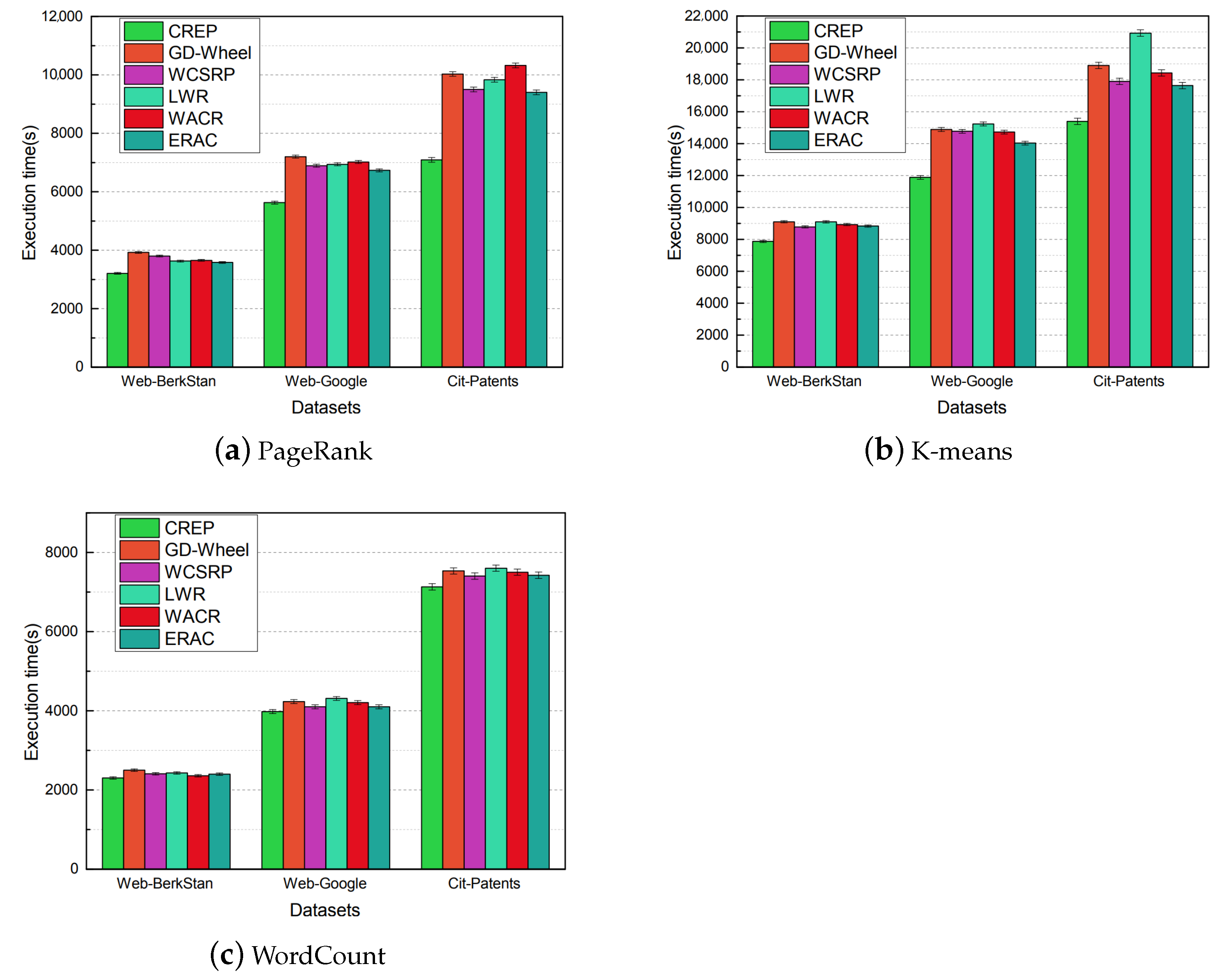[19] considered the partition size, storage time, usage times and calculation cost to design a new weight replacement algorithm. The experimental results showed that the execution time of jobs was obviously improved. Liu et al. [20] analyzed the architecture of Spark and confirmed that the location attributes of the partitions were vital to the cache replacement algorithm. Then, a location-aware cache replacement algorithm was proposed, called WCSRP, considering the location attributes of the partitions. Bian et al. 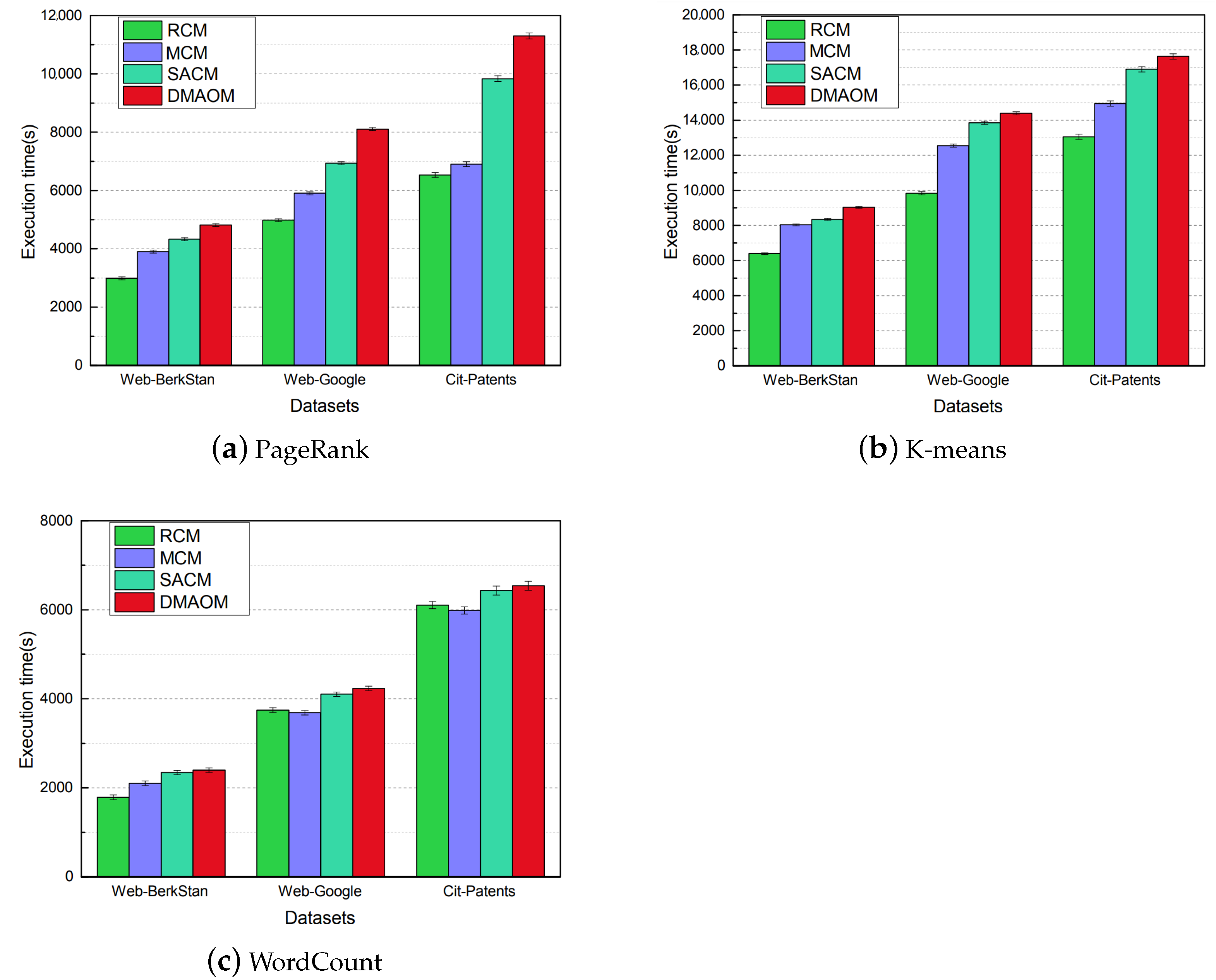[21] designed a method to collect the frequency of RDD and gave a weight of RDD to take the frequency of RDD into consideration. A lowest weight replacement algorithm, called LWR, is proposed. At the same time, they proposed a cache management strategy, called SACM, to reduce the job execution time for Spark. Kun et al. [22] designed an adaptive cache replacement algorithm, called WACR, which takes into account the influence of four weight factors, including computation cost, usage times, partition size and life cycle of RDDs by reasonably calcuting the RDD partition weight values. Wei et al. [23] propose an efficient RDD automatic cache algorithm, called ERAC, to distinguish the high reused RDD and set different degrees to replace old RDD. SuzhenWang et al. [24] propose the implementation of memory on-demand allocation algorithm, called DMAOM, and according to the task request memory size proportionally allocate memory from the resource pool. The weight is proportional to the cache hitting rate. In a limited time scope, the cache hitting rate is high. However, as time passed, the hitting rate become low. These works ignore the time loss of weight during the job running, which leads to a low hitting rate to some degree. Song et al. [25] insisted that the optimization of cache replacement is limited when the memory is severely insufcient. An advanced memory management method is proposed, called MCM, to improve performance by reducing contention. Compared to similar works, MCM reduces the execution time by 28.3%.

The cache data placement problem is similar to the virtual machine placement problem (VMP), and the related placement strategies have great guiding significance [26,27]. A virtual machine (VM) is a computer with a logically specific resource configuration. A physical machine (PM) refers to the computer configured by physical hardware resources. Actually, VMs run on the PMs. VMP refers to assigning a group of VMs to PMs using placement strategies to improve service efficiency. Recently, the research of VMP focuses on two aspects: the optimization of the matching algorithm and the definition of the objective function. For optimization of the matching algorithm, many mathematical optimization techniques are put to use. Hui Zhao et al. 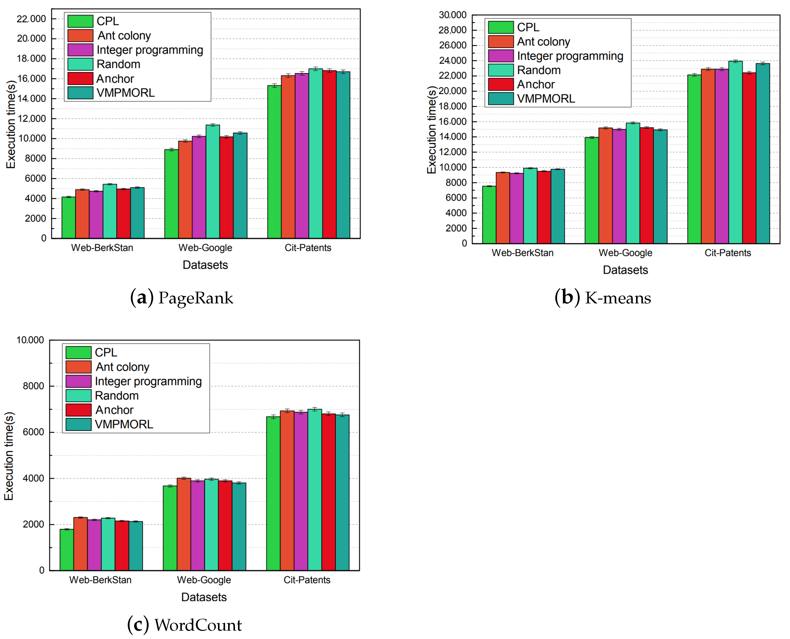[28] proposed an algorithm based on ant colony to minimize PM power consumption and guarantee VM performance. Ye et al. [29] adopted an Integer Programming Model to minimize the number of PMs. Xu et al. [30] proposed a new many-to-one stable matching theory, called Anchor, that efficiently matches VMs with heterogeneous resource needs to servers. For the definition of objective function, Qin et al. [31] proposed a multi-objective virtual machine (VM) placement method, called VMPMORL, to minimize energy consumption and resource wastage simultaneously. Riahi et al. [32] propose an efficient framework based on multi-objective genetic algorithm and Bernoulli simulation that aims to minimize simultaneously used hosts and resource wastage in each PM of the cloud computing platform. Mann et al. 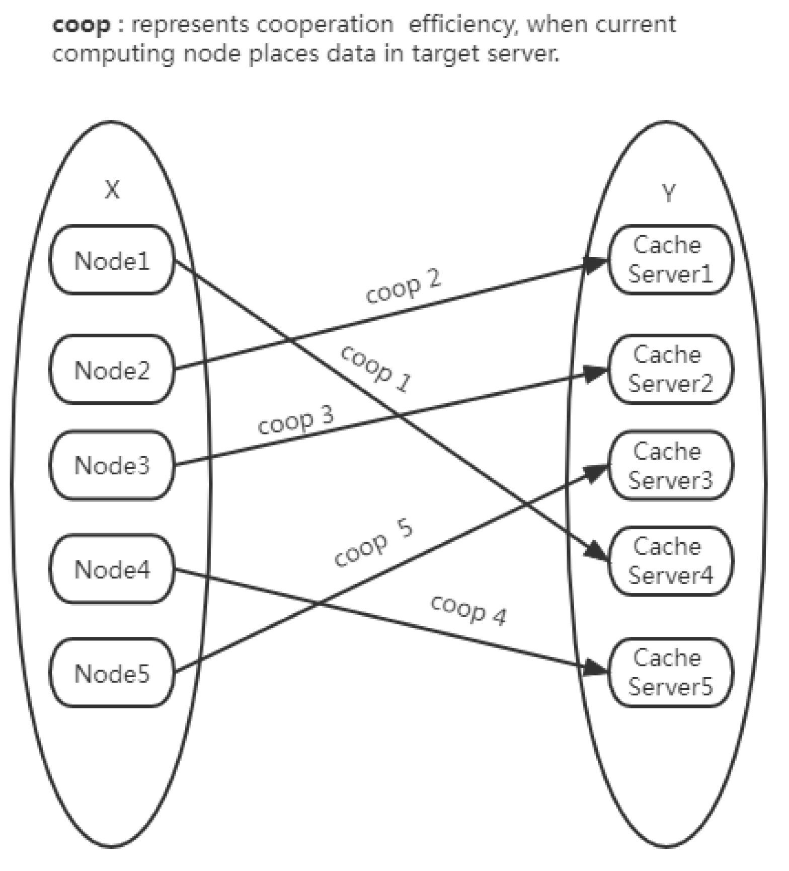[33] argue that it is necessary to simplify the model of scheduling issues. Then, they propose a multicore-aware virtual machine placement algorithm by constraint programming techniques. From what has been discussed aboved, they give different target functions and search algorithms to find the best match. However, the target function ignores the cooperation efficiency between computing node and cache servers. It is a key to measure which server is efficient. These search algorithms make it difficult to find the optimal solution in bipartite graph. The cache data placement problem can draw lessons from these research studies of VMP. However, the definition of thet objective function and more efficient matching algorithm need to be further explored in our study.

3. Problem Analysis and Modeling

In this section, we firstly describe the process of quering data when the cache layer is added. When the cache resource is insufficient, we give a data weight generation model to measure which data are important. Then, the cache replacement model gives the objective function to save important data as much as possible. In the end, we give the coopertion efficiency model to measure which server should be selected when the data are saved.

The process of quering data is shown in Figure 2. After the user initiates a query request, the database query task is created. Firstly, the request obtains the query results from the specified database servers. Secondly, because some results will be queried repeatedly, the important results are written in the remote cache servers. Thirdly, when the result is queried again, the request is sent to the remote servers and the cache server returns results, which has a higher I/O speed.

3.1. Data Weight Generation Model

In the actual process, the result could be from multiple data blocks. After the user initiates a query, different database servers will be accessed. The query of separate servers can be as a sub-request. Then, let $Query=\{SubReq1,SubReq2,\dots ,SubReqk\}$ be a set of sub-requests of a query. Because all the sub-requests are parallel execution, the response time of the result is the longest time of sub-requests. Therefore, the response time of the result is formalized as shown in Equation (1).

$$T_{Query}=Max(T_{SubReq1},T_{SubReq2},...;T_{SubReqk})$$

(1)

where $T_{SubReq1}$ represents the response time of the first sub-request,$T_{SubReq2}$ represents the response time of the second sub-request, $T_{SubReqk}$ represents the response time of the k-th sub-request. In a period of time, the result may be queried repeatedly. The number of queries is defined as NumQ; then, the total time cost of quering the result is shown in Equation (2).

$$T_{cost}=NumQ\times T_{Query}$$

(2)

Because the I/O speed of the remote cache server is higher than that of the database server, if the result is hit, the time of querying the result will be reduced. Therefore, the total time cost of querying the result is a positive factor when we consider which should be remained. On the contrary, the data size is a negative factor for the sake of the limited cache resource. The larger the data size, the fewer free resources there are. In the end, the original weight is shown in Equation (3).

$$weight\_ori=\frac{T_{cost}}{size}$$

(3)

where size represents the data size, and $T_{cost}$ represents the total time cost of querying the result. By monitoring a large number of jobs, we found that the old data have a lower hit probability than before in the cache. So, the time loss of $weight\_ori$ can be described with a time loss function. In the weight generation model, the time loss function is designed as shown in Equation (4).

$$F(weight\_ori)=weight\_ori\times exp\frac{-y\times (t_{last}-t_{start})}{T_{recent}}$$

(4)

where y represents an accommodation coefficient to control the influence of time loss, $t_{start}$ represents the time saved in the cache, $t_{last}$ represents the last time of hitting the cache, and $T_{recent}$ represents the time interval, which is from saving in cache to now.

3.2. Cache Replacement Model

Cache resources are always scarce in computer system architecture. The cache replacement model will clean data of low weight to retain the data of high weight. In the case of limited cache resources, the cache replacement model ensures the maximum data weight of cache space to enhance the hit probability. The total size of cache resources is defined as MaxSpace. In the end, the cache replacement optimization problem can be defned as Equation (5).

$$\begin{array}{c}\hfill Max(\sum _{i=1}^k{F}_i(weight\_ori))\\ \hfill s.t.\sum _{i=1}^{k}siz{e}_i<MaxSpace\end{array}$$

(5)

where ${\sum }_{i=1}^k{F}_i(weight\_ori)$ represents the sum of weight of cache data, MaxSpace represents the total size of cache resources, and ${\sum }_{i=1}^{k}siz{e}_i$ represents the sum of cache data. As we can see from Equation (5), the definition of cache replacement optimization problem includes two parts. The nether part is a constraint condition. It limits the number of cache data to meet resource requirement that the sum of cache data is within the total memory space. The upper part is the objective function to maximize the sum of weight of the cache data.

3.3. Coopertion Efficiency Model

The network architecture of remote cache servers is shown in Figure 3. To avoid frequently querying databases, the important result will be cached in a remote cache server. When the same result is queried again, the computing node will directly request the remote cache server. However, different target servers have different efficiencies.

At the same time, because the job of running on computing nodes and saving cache data in cache servers give dynamic load to computing resources and transmission resources, the computing capacity and transmission capacities of servers become dynamic. To place cache data to the best cache server, the measure of the cooperation efficiency of computing node and remote cache server is established.

Let $CNode=\{nod{e}_1,nod{e}_2,\dots ,nod{e}_m\}$ be a set of computing nodes. Let $CServer=\{serve{r}_1,serve{r}_2,\dots ,serve{r}_n\}$ be a set of cache servers. The $nod{e}_i$ represents a computing node from $CNode$. The $serve{r}_j$ represents a cache server from $CServer$. The processing speed of the cache server represents the computing ability of $serve{r}_j$. Assuming that the size of a dataset is defined as $SD$, the execution time of the job, which loaded the same dataset, is defined as $T_{cache\_j}$. Then, the processing speed is shown in Equation (6).

$${\lambda }_{comp\_j}=\frac{SD}{T_{cache\_j}}$$

(6)

The I/O speed in the network represents transmission efficiency. The transmission time of the dataset from $nod{e}_i$ to $serve{r}_j$ is defined as $T_{tran\_ij}$. Then, the I/O speed is shown in Equation (7).

$${\lambda }_{tran\_ij}=\frac{SD}{T_{tran\_ij}}$$

(7)

Exactly, the processing data and transmission data are the succession of two stages, when saving the data to servers. The cooperation efficiency takes the processing speed and the I/O speed into consideration. Then, the cooperation efficiency is shown in Equation (8).

$${\lambda }_{coop\_ij}={\lambda }_{comp\_j}+{\lambda }_{tran\_ij}$$

(8)

where i indicates the subscript of computing nodes and j indicates the subscript of the cache servers.

In order to make full use of cache resources, the data of computing node are assigned to the most efficient server in priority. According to the measure of cooperation efficiency, the optimization objective function can be formalized as shown in Equation (9).

$$\begin{array}{c}\hfill Max\left(\sum _{i=1}^m\sum _{j=1}^n{\lambda }_{coop\_ij}\right)\\ \hfill s.t.i<m\\ \hfill j<n\end{array}$$

(9)

4. Framework Implementation

In Section 4, we expound the detail of RCM implementation. Firstly, in Section 4.1, we generally introduce the architecture of RCM. Then, in Section 4.2 and Section 4.3, CWG and CREP are proposed to solve the problems of data weight generation and cache replacement. In the end, CPL is designed to solve the problem of cache data placement.

4.1. Overall Architecture of the Framework

The overall flowchart of RCM is shown in Figure 4. Firstly, the system service module represents the source of querying. System users directly interact with this module, and queries are created by the module. Secondly, the status monitor and data collection module monitor the performance of the job. Some basic data are collected by this module, including the response time of the query database, the number of queries, the data size and cooperation efficiency. These data are recorded in a hash table. Thirdly, the weight generator module obtains the data weight according to CWG and generates a candidate list. Then, the candidate list is pushed to a cache placement module and cache replacement module. Fourthly, the cache placement module calculates the cooperation efficiency of the candidate data according to Equation (8) and then stores it in the best cache server. In addition, CPL will calculate the priority of different servers dynamically according to the formula of cooperation efficiency. In a priority list, if the best server does not have enough space and the second server does, the second server will be updated as the best server. Until all servers do not have enough space, the CREP will remove cache data of low weight and store the higher weight data from the candidate list.

4.2. Cache Data Weight Generation Module

CWG implements the function of the weight generation module. According to Section 3.1, CWG takes the response time of the query database, the number of queries, the data size and time loss into consideration. At the beginning, the original weight is obtained by the form of a cost ratio. To introduce the characteristic of time loss, a time loss function is given, which mirrors that the hit rate is reduced with the lapse of time. The final weight is obtained by the time loss function. Then, a candidate list is created by the weight sorting. According to Section 4.1, the basic data are collected by a status monitor and data collection module.

The pseudocode of CWG is shown in Algorithm 1. When a new database query is sent, QueryReq is given a non-null value, and the weight starts to be calculated (line 1). Firstly, basic variables are initialized (line 2 to line 4). The free space, RestSpace, is set to MaxSpace, which is the maximum value of cache resources. The response time of querying, $T_{Query}$, is set to 0. The time cost of totally querying data, $T_{cost}$, is set to 0. Then, basic data are extracted from QueryReq (line 5 to line 15). The saving time of data, $t_{start}$, is recorded if the data do not exist in the cache. The frequency of querying data adds one. Data size, size, is recorded. $T_{Query}$ records the longest response time for sub-requests, while $T_{cost}$ records the total time cost for current data. According to Equation (3), $weight\_ori$ is calculated (line 16). According to Equation (4), weight, which has taken time loss into consideration, is obtained (line 18). As a result, the weight and QueryReq are recorded in the candidates list (line 19). In the end, we give the analysis of complexity. CWG has two nested loops. Therefore, it has a time complexity of O (N). Due to the weight and QueryReq being recorded in the candidates list, which is two-dimensional, the space occupation of CWG is O ($N^2$).

Algorithm 1 CWG Algorithm.

Input:  y: is an accommodation coefficient to control the influence of time loss; $HashMap<queryId,frequency>TaskList$: is a list of recording frequency for every query; $RestSpace$: represents the size of free space in the cache; $MaxSpace$: represents the total size of cache space; $QueryReq$: is a request wrapper;

Output:$List<QueryReq,weight>candidates$: is the candidates data for saving in cache;

1: while $QueryReq!=NULL$do 2:     $RestSpace=MaxSpace$; 3:     $T_{Query}=0$; 4:     $T_{cost}=0$; 5:     if $TaskList\left[QueryREquationqueryId\right]==NULL$ then 6:         $t_{start}=current.time$; 7:     end if 8:     $++TaskList\left[QueryREquationqueryId\right]$; 9:     $size=QueryREquationsize$; 10:     for $i=0toQueryREquationsubQuery.length-1$ do 11:         if $QueryREquationsubQuery\left[i\right].time>T$ then 12:            $T_{Query}=QueryREquationsubQuery\left[i\right].time$; 13:         end if 14:     end for 15:     $T_{cost}=TaskList\left[QueryREquationqueryId\right]\times T_{Query}$; 16:     $weight\_ori=\frac{T_{cost}}{size}$; 17:     $t_{last}=current.time$; 18:     $weight=weight\_ori\times \frac{-y\times (t_{last}-t_{start})}{T_{recent}}$; 19:     $candidates.add(QueryReq,weight)$; 20: end while

4.3. Cache Replacement Module

When the memory space of the cache server is insufficient, the cache replacement algorithm replaces low weight data with high weight data to maximize the sum of cache weights. According to the objective function Equation (5), it can be seen that this problem is a non-linear integer programming problem. It is difficult to obtain an accurate solution in polynomial time. Based on the greedy algorithm, CREP finds the optimal solution in the current round and obtains an approximate solution through an iteration process. Then, CREP is described in detail.

The sub-problem of Equation (5) can be described as follows: Firstly, cache data of the lowest weight are removed. Then, the data of the candidate list are sorted by weight. Let $F_{1th}$ be the first data weight of candidate list. Let $F_{2th}$ be the first two data weights of the candidate list. Let $F_{3th}$ be the first three data weights of the candidate list, and so on; let $F_{kth}$ be the first k data weight of the candidate list. According to the principle of the greedy algorithm, cache servers store as many candidate data as possible within the size of the cache resource. Therefore, the sub-problem is defned as shown in Equation (10).

$$\begin{array}{c}\hfill Max(F_{1th},F_{2th},F_{3th},...;F_{kth})\\ \hfill s.t.\sum _{i=1}^{k}CandidateSiz{e}_i<RestSpace\end{array}$$

(10)

where RestSpace represents free cache resource before the replacement operation, and $CandidateSize$ represents the size of candidate data. The sub-problem is solved after a round of cache replacement. Then, the solutions of all the sub-problems are merged to form the final solution set. The pseudocode of CREP is shown in Algorithm 2.

Algorithm 2 CREP Algorithm.

Input:  $RestSpace$: represents the size of free space in the cache; $MaxSpace$: represents the total size of cache space; $cacheDataList$: records cached data; $QueryReq$: is a request wrapper; $List<QueryReq,weight>candidates$: is the candidates data for saving in cache;

1: CWG (); 2: cacheDataList.orderByWeight (); 3: candidates.orderByWeight (); 4: while candidates.notEmpty () do 5:     Remove (cacheDataList [cacheDataList.length-1]); 6:     for i = 0 to $candidates.length$-1 do 7:         if candidates[i][0].size < restSpace then 8:            Save (candidates[i][0].data ); 9:         end if 10:     end for 11: end while

If the cache resource is insufficient, CREP starts to work. At first, some pretreatments are performed (line 1 to line 3). The candidate data list can be obtained from the return result of the CWG algorithm. In order to accelerate the replacement operation, cacheDataList and candidates are sorted by weight. Then, candidate data try to replace low weight data in the cache. The process of replacement follows: Firstly, CREP removes the data of the lowest weight from cacheDataList. Secondly, CREP tries to transfer the highest weight data from the candidates list to cache. Thirdly, the first two steps are repeated until the candidates list is empty (line 4–line 11). In the end, we give the analysis of complexity. CREP also has two nested loops. So, it has the time complexity of O ($N^2$). The space occupation of CREP has two parts, cacheDataList and candidates. They also are two-dimensional. However, the address of candidates is pointing to the address of the candidates list of Algorithm 1. It shared data in two algorithms. Therefore, Algorithm 2 has the space complexity of O ($N^2$).

4.4. Cache Placement Module

The computing nodes initiate a query for the cache server, and the cache server is responsible for responding to the query. Because of the computing and transmission process, different servers have different cooperation efficiencies for every computing node. According to Equation (9), the goal of the cache placement problem is to maximize the cooperation efficiency between computing nodes and servers. This problem is described as maximum weight matching in bipartite graph G = (V, E). In Figure 5, the left vertexes set of the bipartite graph, named X, represents the computing nodes and the right vertexes set of the bipartite graph, named Y, represents the cache servers. The edges, which connect X to Y, represent cooperation efficiency with weight.

In order to solve the maximum weight-matching problem in a bipartite graph, we adopt the Kuhn-Munkres (KM) algorithm [1] to find optimal solution. We define the items $TX$ (i) and $SY$ (j) for every $i\in X$ and $j\in Y$. If the $edg{e}_{ij}$ meets the condition that $TX$ (i) + $SY$ (j) ≥ $weigh{t}_{ij}$, these items are called “feasible”. Let G be divided into different subgraphs. G* = (V, E*) is called “the equality subgraph” only when all the edges of G* meet the condition that $TX$ (i) + $SY$ (j) = $weigh{t}_{ij}$. When M’ meets the condition that all vertices in X have been matched to Y, M’ is called “the perfect matching” in G*.

Theorem 1. 

Given feasible items, if there is M’ in G*, M’ is also the optimal matching for G.

Proof of Theorem 1. 

Let P be equal to ${\sum }_{i\in X}TX\left(i\right)+{\sum }_{j\in Y}SY\left(j\right)$. For all feasible items, the sum of all weights always meets $\sum weigh{t}_{ij}\le P$. If matching M meets the condition that $\sum weigh{t}_{ij}=P$, M is the optimal matching. Then, considering the perfect matching M’, the weight of any edge meets the condition that $TX$ (i) + $SY$ (j) = $weigh{t}_{ij}$. So, the sum of all weights meets the condition that $\sum weigh{t}_{ij}=P$, which means that M’ is also the optimal matching for G.   □

Based on Theorem 1, our goal is to find M’ in G*. The KM algorithm searchs the augmenting path in G* to find a perfect match. If a perfect match is not found, some items of vertices are adjusted and add more edges to G*. CPL uses the KM algorithm to find the best match. In detail, we describe the procedures in Algorithm 3.

Algorithm 3 KM Algorithm.

Input:  $List<taskId>TX$: represents the item of the cache; $List<serverId>SY$: represents the item of servers; $List<flag>vistTX$: is the flag of visiting left vertices; $List<flag>vistSY$: is the flag of visiting right vertices; $List<taskId,serverId>efficiencyList$: is a list of recording cooperation efficiency between computing nodes and cache servers;

Output:$match\left[i\right]$: is the best matching result;

1: for i = 0 to N − 1 do 2:     TX[i] = max (efficiencyList[i][j]), SY[i] = 0, match[i] = −1; 3: end for 4: for i = 0 to N − 1 do 5:     for j = 0 to N − 1 do 6:         slack[j] = INF; 7:         while TRUE do 8:            for j = 1 to N do 9:                vistTX[i] = FALSE, vistSY[i] = FALSE; 10:                if FindPath (i) then 11:                    break; 12:                else 13:                    $\varphi$ = min (slack[j] ); 14:                end if 15:            end for 16:            for j = 1 to N do 17:                vistTX[i] = FALSE, vistSY[i] = FALSE; 18:                if vistTX[j] then 19:                    TX[j] = TX[j] −$\varphi$; 20:                else if vistSY[j] then 21:                    SY[j] = SY[j] −$\varphi$; 22:                else 23:                    Slack[j] = Slack[j] −$\varphi$; 24:                end if 25:            end for 26:         end while 27:     end for 28: end for

In the bipartite graph, TX represents the item of cache, and SY represents the item of servers. vistTX and vistSY represent the flag of visiting. efficiencyList records the cooperation efficiency between the nodes and servers. Firstly, to promise items TX and SY are feasible, TX is initialized to the maximum value of weight. SY is initialized to 0, and match[i] is initialized to −1 (line 2). Then, the augmenting path of G* is searched to try to find the best matching (line 4 to line 11). Because of lacking enough edges, it is possible that there is not perfect matching in G*. In order to add more edges, the gap of items is narrowed between TX and SY (line 16 to line 25). After the adjustment, some edges will be added to G* while promising all the items are feasible. Then, the augmenting path of G* is searched repeatedly until the perfect matching is found.

The process of searching is shown in Algorithm 4. FindPath (i) visits the vertices, i, to find the matching of meeting $TX$ (i) + $SY$ (j) = $weigh{t}_{ij}$ (line 1 to line 6). If that is met, FindPath (j) is run to try to search the augmenting path of G* (line 7 to line 9). When the augmenting path meets $\sum weigh{t}_{ij}={\sum }_{i\in X}TX\left(i\right)+{\sum }_{j\in Y}SY\left(j\right)$, the perfect matching is found in G*.

Algorithm 4 Find Path.

1: vistTX[i] = True; 2: for j = 1 to N do 3:     if vistDY[j] then 4:         continue; 5:     end if 6:     $\varphi$ = TX[i] + SY[ j ] – efficiencyList[i][j]; 7:     if $\varphi$ == 0 then 8:         vistSY[j] = TRUE; 9:         if match[j] == −1 or findpath (match[j]) then 10:            match[−1] = i; 11:            return TRUE; 12:         end if 13:     else if slack[j] >$\varphi$ then 14:         slack[j] = $\varphi$; 15:     end if 16: end for 17: return FALSE;

In the end, we analyze the complexity of CPL. According to Algorithm 3, CPL has three nested loops. Therefore, it has a time complexity of O ($N^3$). The scale of time complexity depends on N. Due to the limited remote cache servers, N will not be very large. So, there will be no time efficiency explosion. The space occupation of CPL is the two-dimensional cooperation efficiency table. It has a space complexity of O ($N^2$).

5. Experimental Results and Analysis

In this section, we describe the relevant experimental environment, benchmark workloads and performance metrics during the experiment. Then, we test CREP and CPL individually. Finally, we analyze the experimental results and evaluate the performance of RCM.

5.1. Experimental Setup

In order to validate the effectiveness of RCM during jobs execution, RCM is implemented on Reids as a service of remote cache. The Spark platform will run benchmark jobs to test performance of RCM. The experiment starts eight computing nodes and four cache servers. The configuration of the experiment environment is shown in

Table 1. Resource configuration information.

Parameter	Configuration
CPU	Intel (R) Xeon (R) Platinum 8160 CPU @ 2.10 GHz
RAM	64G
Hard Disk	1TB
OS	CentOS 7.0
Spark	Cloudera Spark 2.4.0-cdh6.2.1
Cloudera Manager	CDH 6.2.1
Yarn	Yarn-3.0.0
Redis	Redis 5.0
JDK	JDK 8.0
HDFS	HDFS 2.0.0

. HDFS is chosen as the database service. The benchmark jobs include PageRank, K-means and WordCount. The benchmark workloads of jobs are shown in

Table 2. Benchmark workloads.

Job Type	Iteration Rounds
PageRank	3000
K-means	5000
WordCount	1

. The main metric of the experiment is the job execution time. Provided by SNAP [34], three standard datasets, Web-BerkStan, Web-Google and Cit-Patents, are selected. To increase the pressure on cache resources, Web-BerkStan, Web-Google and Cit-Patents are expanded to 500 GB, 1 TB and 2 TB, respectively.

5.2. Performance Result

5.2.1. CREP Performance Improvement

In order to test the effectiveness of CREP, this section sets up three groups of benchmark jobs to observe the acceleration effect. The execution time of benchmark jobs, PageRank, K-means and WordCount, are shown in Figure 6a–c, respectively. Advanced cache replacement algorithms are set, including GD-Wheel [15], WCSRP [20], LWR [21], WACR [22] and ERAC [23].

In Figure 6a, the X-axis represents the type of datasets and the Y-axis represents the execution time. For Web-BerkStan and Web-Google, the execution time of GD-Wheel has the longest and CREP has the shortest. As the size of the dataset increases, it is obvious that the execution time of CREP is shorter than that of the other algorithms. For Cit-Patents, the execution time of WACR has the longest and CREP has the shortest. CREP reduces the job execution time compared with GD-Wheel, WCSRP, LWR, WACR and ERAC by an average of 28.9%, 24.2%, 25.8%, 26.1%, and 22.5%, respectively. That is because the CREP considers not only the response time of the query database, the number of queries, and the data size but also the time loss of weight during job running, which accelerates the job. In Figure 6b, the best performance of CREP is further verified. In Figure 6c, WordCount, a computation-intensive job hardly has a better optimization than PageRank and K-means. Combined with source code to analyze this phenomenon, we can conclude that WordCount has less interaction with cache resources than PageRank and K-means. So, it is insensitive to cache pressure. From what has been discussed above, it is revealed that CREP has a perfect optimization for the jobs which are not computation-intensive.

5.2.2. CPL Performance Improvement

This section verifies the effectiveness of CPL by three groups of benchmark jobs. At the same time, advanced matching optimization algorithms are compared, including ant colony [28], integer programming [29], Random, Anchor [30] and VMPMORL [31]. In particular, Random, which is a random matching algorithm, is tested as the original condition. The execution times of benchmark jobs are shown in Figure 7a–c, respectively.

In Figure 7a, the X-axis represents the type of datasets and the Y-axis represents the execution time. For Web-BerkStan, CPL has the shortest time. Compared to Random, CPL reduces the execution time by 27.2% at most. As the size of the dataset increases, the execution time becomes long. For Web-Google and Cit-Patents, two larger datasets, these have less optimization than Web-BerkStan. In Figure 7b, for Web-BerkStan, CPL gives a 10% improvement of the K-means job base on random algorithms. As the size of the dataset increases, the rate of improvement reduced by 8.3%. In Figure 7c, the best performance of CPL is further verified. CPL reduces the execution time compared with ant colony by 18.3% for Web-BerkStan. From what has been discussed above, CPL can reduce execution time effectively; this is because the cooperation efficiency is the best measure to find the most efficient servers. In addition, the result also proves that the KM algorithm is suitable to the problem of cache data placement. However, we finds that an insufficient cache resource reduces the performance of CPL. In Figure 7a, for Web-BerkStan, CPL gives about a 27.2% improvement of the K-means job base on random algorithms. As the size of the dataset increases, there is a downward trend on the rate of improvement. For Web-Google and Cit-Patents, the improvement of CPL reduces by 11.5% and 8.3%, respectively. The downward trend is also shown in Figure 7b,c. Analyzing this phenomenon, the size of the dataset is the main influencing factor. Web-BerkStan, Web-Google and Cit-Patents are expanded to 500 GB, 1 TB and 2 TB, respectively, so the cache pressure is increasing gradually. For Web-BerkStan, the server load is unbalanced. CPL plays a role as a dynamic load balancer to reduce the execution time. However, for Web-Google and Cit-Patents, all servers are high load status. The load balancer does not have the obvious acceleration effect.

5.2.3. RCM Performance Improvement

CREP and CPL have been tested individually in Section 5.2.1 and Section 5.2.2. This section verifies the effectiveness of RCM, which consists of CREP and CPL. Firstly, advanced cache management strategies of Spark, including MCM [25], SACM [21] and DMAOM [24], are tested to compare the performance of RCM.

The execution time of benchmark jobs, PageRank, K-means and WordCount, are shown in Figure 8a–c, respectively. For Web-Google in Figure 8a, RCM gives a 28% improvement of PageRank job at most. For Cit-Patents in Figure 8b, RCM gives a 42.1% improvement of K-means job at most. For Web-BerkStan in Figure 8c, RCM gives a 16.8% improvement of the WordCount job at most. The results of the three jobs confirm that RCM has the most obvious optimization compared with the other strategies. However, RCM has less optimization on computation-intensive jobs. In Figure 8c, the execution time of three datasets shows that RCM is not in a dominant position. For Cit-Patents in Figure 8c, RCM does not perform as well as MCM does. Analyzing this phenomenon to reveal the best type of scenario in which RCM can achieve the most optimization, we can make a classification according the frequency of accessing memory. PageRank and K-means are input and output intensive for cache resources, while WordCount is not. The job type of input and output intension has obvious acceleration by optimizing cache management; this is why RCM has a dominant position in PageRank and K-means. On the contrary, WordCount is less affected by cache management optimization. It is difficult to reduce the execution time from the view of optimizing cache management. In the end, we conclude that the best type of scenario in which RCM can achieve the most optimization is an input and output-intensive scenario, which is accessing cache resource frequently.

6. Conclusions

To solve the problem of cache management optimization of a big data platform, we propose RCM, a remote cache management framework for Spark, including a cache data weight generation module (CWG), cache replacement module (CREP), and data placement module (CPL). CWG establishes a new cache data weight model according to the task characteristics of the big data platform. The initial weight is obtained by considering the response time of the query database, the number of queries, and the data size. Then, the time loss function is given to define the weight change caused by time loss. CREP uses the weight generated by CWG to define the priority of cache replacement. When cache resources are insufficient, low-priority cache data are replaced by high-priority data. CPL dynamically matches the best cache server based on the KM algorithm to improve cooperation efficiency. To verify the effectiveness of RCM, we implement RCM based on Redis and deploy it on eight computing nodes and four cache servers. Three kinds of experimental datasets are selected from SNAP [34] datasets, and the benchmark jobs are PageRank, K-means and WordCount. The experiment proves that RCM has a more obvious cache acceleration effect on the big data platform than advanced cache management strategies. Compared with MCM, SACM and DMAOM, the execution time of RCM is reduced by 42.1% at most.

Because RCM is independent from the Spark platform, it is easy to perform a remote cache management component in other big data platforms. In the future work, we wil try to deploy RCM on other big data platforms, such as Hadoop [35], Flink [36], and Storm [37].

References

1. Ahmed, N.; Barczak, A.; Susnjak, T.; Rashid, M.A. A comprehensive performance analysis of Apache Hadoop and Apache Spark for large scale data sets using HiBench. J. Big Data 2020, 7, 167–182. [Google Scholar] [CrossRef]
2. Xu, L.; Li, M.; Zhang, L.; Butt, A.R.; Wang, Y.; Hu, Z.Z. MEMTUNE: Dynamic memory management for in-memory data analytic platforms. Proc. IEEE Int. Parallel Distrib. Process. Symp. 2016, 91, 383–392. [Google Scholar]
3. Tsai, C.P.; Chang, C.W.; Hsiao, H.C.; Shen, H. The Time Machine in Columnar NoSQL Databases: The Case of Apache HBase. Future Internet 2022, 14, 583–599. [Google Scholar] [CrossRef]
4. Nicholson, H.; Chrysogelos, P.; Ailamaki, A. HPCache: Memory-Efficient OLAP Through Proportional Caching. In Data Management on New Hardware. Assoc. Comput. Mach. 2022, 7, 125–134. [Google Scholar]
5. Harrison, G. Redis and Amazon’s MemoryDB. Database Trends Appl. 2021, 35, 5. [Google Scholar]
6. Wang, S.; Zhang, Y.; Zhang, L.; Cao, N.; Pang, C. An Improved Memory Cache Management Study Based on Spark. Comput. Mater. Contin. 2018, 56, 415–431. [Google Scholar]
7. Geng, Y.; Shi, X.; Pei, C.; Jin, H.; Jiang, W. LCS: An Efficient Data Eviction Strategy for Spark. Int. J. Parallel Program 2017, 45, 1285–1297. [Google Scholar] [CrossRef]
8. Chenyang, Z. Design and Implementation of Distributed Cache for Heterogeneous Multilevel Strorage. Ph.D. Thesis, University of Electronic Science and technology, Chengdu, China, 2022. [Google Scholar]
9. Robinson, J.T.; Devarakonda, M.V. Data cache management using frequency-based replacement. ACM Sigmetrics Perform. Eval. Rev. 1990, 16, 1353–1365. [Google Scholar]
10. Apache. Apache Spark Web Interfaces. Available online: https://Spark.apache.org/docs/latest/monitoring.html (accessed on 24 June 2022).
11. Hong-Tao, M.; Song-ping, Y.; Fang, L.; Nong, X.I.A.O. Research on Memory Management and Cache Replacement Policies in Spark. Comput. Sci. 2017, 80, 37–41. [Google Scholar]
12. Edmonds, J. Maximum matching and a polyhedron with 0, 1 vertices. J. Res. Nat. Bur. Stand. B 1965, 69, 55–56. [Google Scholar] [CrossRef]
13. Jia, B.; Li, R.; Wang, C.; Qiu, C.; Wang, X. Cluster-based content caching driven by popularity prediction. CCF Trans. High Perform. Comput. 2022, 4, 357–366. [Google Scholar] [CrossRef]
14. Cai, R.Y.; Qian, Y.; Wei, D.B. Dynamic Cache Replacement Strategy of Space Information Network Based on Cache Value; IOP Publishing Ltd.: Bristol, UK, 2022. [Google Scholar]
15. Li, C.; Cox, A.L. GD-Wheel A cost-aware replacement policy for key-value stores. In Proceedings of the Tenth European Conference on Computer Systems ACM, Bordeaux, France, 21–24 April 2015; pp. 1–15. [Google Scholar]
16. Xuan, T.N.; Thi, V.T.; Khanh, L.H. A Design Model Network for Intelligent Web Cache Replacement in Web Proxy Caching. Intell. Syst. Netw. 2022, 471, 235–249. [Google Scholar]
17. Long, F. A Cache Admission Policy for Cloud Block Storage Using Deep Reinforcement Learning. Int. Conf. Comput. Ind. Eng. 2022, 920, 462–469. [Google Scholar]
18. Ruan, J.; Xie, D. Content-Aware Proactive VR Video Caching for Cache-Enabled AP over Edge Networks. Electronics 2022, 11, 24–28. [Google Scholar] [CrossRef]
19. Duan, M.; Li, K.; Tang, Z.; Xiao, G.; Li, K. Selection and replacement algorithms for memory performance improvement in Spark. Concurr. Comput. Pract. Exp. 2016, 28, 2473–2486. [Google Scholar] [CrossRef]
20. Heng, L.; Liang, T. New RDD Partition Weight Cache Replacement Algorithm in Spark. J. Chin. Comput. Syst. 2018, 39, 2279–2284. [Google Scholar]
21. Bian, C.; Yu, J.; Ying, C.T.; Xiu, W.R. Self-Adaptive Strategy for Cache Management in Spark. Acta Electron. Sin. 2017, 45, 278–284. [Google Scholar]
22. Jiang, K.; Du, S.; Zhao, F.; Huang, Y.; Li, C.; Luo, Y. Effective data management strategy and RDD weight cache replacement strategy in Spark. Comput. Commun. 2022, 194, 66–85. [Google Scholar] [CrossRef]
23. Yun, W.; Yuchen, D. Research on efficient RDD self-cache replacement strategy in Spark. Appl. Res. Comput. 2022, 37, 3043–3047. [Google Scholar]
24. Wang, S.; Geng, S.; Zhang, Z.; Ye, A.; Chen, K.; Xu, Z.; Cao, N. A Dynamic Memory Allocation Optimization Mechanism Based on Spark. Comput. Mater. Contin. 2019, 61, 739–757. [Google Scholar] [CrossRef]
25. Song, Y.; Yu, J.; Wang, J, He, X. Memory management optimization strategy in Spark framework based on less contention. J. Supercomput. 2022, 80, 132–152. [Google Scholar] [CrossRef]
26. Wang, J.; Gu, H.; Yu, J.; Song, Y.; He, X. Research on virtual machine consolidation strategy based on combined prediction and energy-aware in cloud computing platform. J. Cloud Comput. 2022, 50, 560–573. [Google Scholar] [CrossRef]
27. Xu, Y.; Liu, L.; Ding, Z. DAG-Aware Joint Task Scheduling and Cache Management in Spark Clusters. IEEE Int. Parallel Distrib. Process. Symp. 2022, 378–387. [Google Scholar] [CrossRef]
28. Zhao, H.; Wang, J.; Liu, F.; Wang, Q.; Zhang, W.; Zheng, Q. Power-aware And performance-guaranteed virtual machine placement in the cloud. IEEE Trans. Parallel Distrib. Syst. 2018, 29, 1385–1400. [Google Scholar] [CrossRef]
29. Ye, K.; Wu, Z.; Wang, C.; Zhou, B.B.; Si, W.; Jiang, X.; Zomaya, A.Y. Profiling-based workload consolidation and migration in virtualized data centers. IEEE Trans. Parallel Distrib. Syst. 2014, 26, 878–890. [Google Scholar] [CrossRef]
30. Xu, H.; Li, B. Anchor: A versatile and efficient framework for resource management in the cloud. IEEE Trans. Parallel Distrib. Syst. 2013, 24, 1066–1076. [Google Scholar] [CrossRef]
31. Qin, Y.; Wang, H.; Yi, S.; Li, X.; Zhai, L. Virtual machine placement based on multi-objective reinforcement learning. Appl. Intell. 2020, 50, 2370–2383. [Google Scholar] [CrossRef]
32. Riahi, M.; Krichen, S. A multi-objective decision support framework for virtual machine placement in cloud data centers: A real case study. J. Supercomput. 2018, 74, 2984–3015. [Google Scholar] [CrossRef]
33. Mann, Z.A. Multicore-Aware Virtual Machine Placement in Cloud Data Centers. IEEE Trans. Comput. 2016, 65, 3357–3369. [Google Scholar] [CrossRef]
34. Jure, L. Stanford Network Analysis Project [EB/OL]. 2022. Available online: http://snap.stanford.edu/data (accessed on 11 June 2022).
35. Apache. Apache Hadoop Project Homepage. Available online: https://hadoop.apache.org (accessed on 11 June 2022).
36. Apache. Apache Flink Project Homepage. Available online: https://flink.apache.org/flink-architecture.html (accessed on 11 June 2022).
37. Apache. Apache Storm Project Document. Available online: https://storm.apache.org/releases/2.4.0/index.html (accessed on 13 June 2022).
Figure 1. Adding a cache layer to Spark cluster.
Applsci 12 11491 g001
Figure 2. The process of quering data.
Applsci 12 11491 g002
Figure 3. The network architecture of remote cache servers.
Applsci 12 11491 g003
Figure 4. The flowchart of RCM.
Applsci 12 11491 g004
Figure 5. Maximum weight matching in bipartite graph.
Applsci 12 11491 g005
Figure 6. Job execution time.
Applsci 12 11491 g006
Figure 7. Job execution time.
Applsci 12 11491 g007
Figure 8. Job execution time.
Applsci 12 11491 g008