Research on the Correlation Filter Tracking Model Based on the Deep-Pruned Feature Network

Abstract

Visual tracking is one of the key research fields in computer vision. Based on the combination of correlation filter tracking (CFT) model and deep convolutional neural networks (DCNNs), deep correlation filter tracking (DCFT) has recently become a critical issue in visual tracking because of CFT’s rapidity and DCNN’s better feature representation. However, DCNNs are often complex in structure, which most possibly results in the conflict between the rapidity and accuracy of DCFT. To reduce such conflict, this paper proposes a model mainly including: (1) Based on the pre-pruning network obtained by feature channel importance, an optimal global tracking pruning rate (GTPR) is determined in terms of the contribution of filter channels to tracking response. (2) Based on (GTPR), an alternative convolutional kernel is defined to replace non-important channel kernels, which leads to the further pruning of the feature network. (3) An online updating pruned feature network with a structural similarity index is employed to adapt the model to tracking scene changes. (4) The proposed model was performed on OTB2013; experimental results demonstrate the model can effectively enhance speed with a 45% increment while guaranteeing tracking accuracy, and improve tracking accuracy with a 4% increment when tracking scene changes take place.

1. Introduction

Visual object tracking is an important branch of computer vision, which can be described as the process of estimating the motion trajectory of a target in subsequent frames, provided that the state information (position, size, etc.) of the target is given in the first frame of the tracking sequence [1,2,3,4]. The traditional visual object tracking algorithms mainly include Mean Shift [5], Lucas Kanade [6], Particle filter [7], etc. In 2010, Bolme [8] introduced correlation filtering into the field of object tracking and proposed the MOSSE (Minimum Output Sum of Squared Error) algorithm. The essence of MOSSE is to first construct a correlation filter with the features of the target in the first video frame; then, starting from the second video frame, the filter correlates the features of the target by Fast Fourier Transform (FFT), which is the reason why the tracking speed is so fast. The maximum value of the filter response is the predicted position of the target, and the filter is updated with the predicted position of the target. Based on MOSSE, many kinds of variant algorithms have been proposed, such as Circulant Structure of Tracking-by-Detection with Kernels (CSK) [9], Kernelized Correlation Filters (KCF) [10], Scale Adaptive Multiple Feature (SAMF) [11], to further enhance the MOSSE’s performance. However, most of these variant algorithms extract target features by hand, which lacks flexibility, online performance, and accuracy for feature extraction. Therefore, it is necessary for the tracking based on the correlation filter to have some ways to obtain target features online with high flexibility and accuracy.

CNNs (convolutional neural networks) have been widely studied in the field of image recognition since the introduction of a new deep structure and dropout method by Alexnet proposed by Hinton et al. [12]. Along with its rapid development, CNN has become one of the main techniques [13] in the field of feature extraction because of its strong feature representation ability. Therefore, a deep convolutional neural network combined with correlation filter tracking [8,9,10,11,14] (named Deep Correlation Filter Tracking) is gradually becoming one of the critical issues in the field of visual object tracking [1,2,3,4,15]. Firstly, deep correlation filter tracking takes a deep convolutional neural network as the feature extractor to online extract deep features from video frames by making full use of the powerful feature representation capabilities of CNN; and secondly, the correlation filter is applied to correlate the target features obtained from CNN to predict target positions with high rapidity. The general process of the deep correlation filter tracking model is shown in Figure 1.

Despite many advances in deep correlation filter tracking models and their successful application in related fields, there are still some challenging problems that need to be addressed. For example, (1) deep convolutional neural networks have powerful feature representation capabilities that improve tracking accuracy. However, their large model size, high computational complexity, and high memory resource requirements increase the complexity of the model, as well as the computational burden, which makes it difficult to meet the real-time requirements of object tracking and also hinders its deployment in embedded mobile devices with limited computational and memory resources [16]. (2) In the actual tracking process, the deep convolutional neural network obtained by offline training is difficult to adapt to the changes of environment and target (e.g., changes in illumination, changes in target scale, rotation, background interference, etc. [17]), which restrains the accuracy of target feature extraction and may lead to lower tracking accuracy, thus affecting the tracking performance.

One of the effective ways to solve the above problems is as follows: Firstly, the pruning algorithm is used to lighten the feature network, to compress the size of the model, reduce the computational burden, and reduce the time it takes for the feature network to extract features, to improve the real-time performance of the correlation filter tracking. Secondly, according to the environment and target changes, the pruned feature network is updated in real-time so that the feature network can adapt to the corresponding changes to improve the tracking accuracy.

For online updating of deep convolutional neural networks, common approaches include: fine-tuning the network using the mask of the previous frame sequence [18]; updating the network in a long-term and short-term fashion [19]; capturing changes in the appearance of the target by residual learning and updating the network by a fixed frame interval [20]. Some researchers have also proposed solutions using dynamic networks [21,22]. Most of the above methods for the online updating of deep convolutional neural networks are proposed for specific disturbances and lack good generalizability and robustness. Therefore, considering the multiple disturbances caused by the environment and updating the deep convolutional neural networks in real-time to improve the tracking accuracy is a bottleneck in the implementation of the deep correlation filter tracking model.

Research on convolutional neural network pruning can be divided into fine-grained pruning and coarse-grained pruning. This paper focuses on the coarse-grained pruning task. Coarse-grained pruning is the structured compression of a model at the convolutional kernel or channel level. The core idea is to first evaluate the importance of the convolutional kernels or feature channels. Then, based on a pre-defined pruning rate, all convolutional kernels or feature channels that contribute little to the result are processed using one of three strategies: eliminating all [23]; setting all to zero [24]; or setting all to zero in a non-linear progressive manner [2]. The eliminating all strategy [23] permanently removes the unimportant convolutional kernels in each iteration, which speeds up the training process to some extent, but leads to a great loss of model accuracy. The setting all to zero strategy [24] and setting all to zero in a non-linear progressive manner strategy [2] also prune the convolutional kernels according to their importance. The main difference is that each pruned convolution kernel is still sent into the next training iteration, reducing the accuracy loss of the model. However, the setting all to zero strategy [24] did not consider the association between convolutional kernels and feature maps when measuring the importance of convolutional kernels. Therefore, the setting all to zero in a non-linear progressive manner strategy [2] improved the importance measurement strategy to increase the interpretability of the importance of the convolutional kernels.

No matter which strategy is adopted, the above pruning patterns will determine how to adjust and optimize the pruning rate, and how to choose a pruning strategy after the pruning rate is determined to improve the tracking accuracy, while keeping the real-time performance of the model.

To solve the bottlenecks mentioned above of the deep correlation filter tracking model, and inspired by the motivation mentioned above and based on our existing research results [1,2,3,4,24], we propose a “correlation filter tracking model based on the deep-pruned feature network” in this paper.

2. Related Works

2.1. Deep Convolutional Neural Network Pruning

As mentioned above, structured coarse-grained pruning is the structured compression algorithm, which takes convolutional kernels or channels as the pruning unit to implement the structured compression of a deep convolutional feature network at the convolutional kernel or channel level, without introducing additional sparsity into the network. However, it is inevitable for fine-grained pruning to produce sparsity. It is difficult to train a good pruning model due to sparsity [24]. In addition, it is necessary for dealing with the sparsity to have extra hardware support [25] which is an extra workload for network pruning. Therefore, structured coarse-grained pruning algorithms have gradually become a major research direction in the field of deep convolutional network pruning research in recent years.

Li et al. [23] proposed a CNN acceleration method based on convolutional kernel pruning, using the L1 norm of the matrix to measure the importance of each convolutional kernel and remove the convolutional kernels with low importance, and the corresponding feature maps as a way to reduce the computational cost of the CNN. Liu et al. [26] used the scaling factor γ in Batch-Normalization as a parameter to measure channel importance and added a regular term of γ to the objective function to be able to automatically prune during the network training process. Ye et al. [27] proposed an OT (Optimal Thresholding) pruning algorithm, considering the differences between different convolutional layers and weight distributions. OT algorithm prunes unimportant channels by calculating the optimal threshold layer by layer, which avoids the problem of over- or under-pruning. In most of the pruning strategies described above, the mode of “eliminating all” unimportant convolutional kernels or channels is used, which will inevitably lead to a large loss of model accuracy. To address this problem, He et al. [24] did not use the “eliminating all” strategy when pruning unimportant convolutional kernels, but set the kernels that needed to be pruned in this iteration to zero and continued training these kernels in the next iteration. The obvious advantage of this is that it considers the global information of a single convolutional kernel during the training process, rather than relying solely on the training results of a particular iteration to assess its final degree of importance. The method proposed by He et al. [24] improves the accuracy loss due to “eliminating all”, but the shortcoming is that the importance of the convolutional kernel is measured solely by the information of the kernel itself, without considering the connection between the kernel and the feature map. In addition, the “set all to zero” strategy causes each iteration of training to start from zero, which may affect the computational efficiency of the training process. Chen et al. [2] improved the algorithm based on [24] and proposed the PCIP (pruning deep feature networks using channel importance propagation) pruning algorithm. In this study, we use the “set all to zero in a non-linear progressive manner” strategy to prune the unimportant convolutional kernels, which not only reduces the accuracy loss caused by pruning, but also improves the computational efficiency during the pruning training process. Additionally, the global average pooling of the feature map is used as the basis for measuring the importance of convolutional kernels, which considers the correlation between convolutional kernels and the feature map, and improves the interpretability of the importance of convolutional kernels.

2.2. Online Updating of Feature Network

The feature network of the deep correlation filter tracking model is usually obtained by offline pre-training, and the pre-trained feature network is not modified during the whole tracking process. For more stable tracking scenarios, not modifying the feature network during the tracking process will not have a significant impact on the performance of the tracker. However, in the practical application of object tracking, the tracking scene often changes with factors such as illumination and the motion state of the target. Offline pre-trained feature networks have difficulty adapting to such changes. Similarly, the pruned network based on the offline pre-trained feature network is also difficult to adapt to such changes in the tracking environment, and therefore cannot accurately extract target features, resulting in the performance degradation of the tracker. Therefore, to improve the ability of the feature network to adapt to complex scene changes, one of the effective ways is to optimize the parameters of the feature network through an online update.

Nam et al. [19] used two strategies to update the network online. The first was to action a long-term update of the network after each fixed frame interval. The second was to action a short-term update of the network when the failure of tracking was detected. Song et al. [20] proposed the CREST (convolutional residual learning scheme for visual tracking) algorithm, which captures changes in target appearance in a residual learning manner and updates the network every fixed frame interval. It effectively improves the robustness of the network when the appearance of the target significantly changes. Qiu et al. [28] used “first frame updating”, “interval frame updating”, and “failure updating” to update the network. That is, using the first frame so the network initially learns the characteristics of the current target; using the high-score samples of frames with several intervals to update the network; and using high-score samples to update the network when the tracking fails, which can improve the characterization ability of the network. Most of the above methods use fixed intervals to update the network. Although they can partially solve the network adaptability problem, the algorithm lacks flexibility and universality, and cannot completely solve the actual adaptability problem in the tracking process. Unlike fixed-interval updating strategies, Yang et al. [3] used SSIM to determine the similarity of tracking boxes in two consecutive frames in real-time during the tracking process, and only updated the feature network when SSIM was below a certain threshold. This not only considers the disturbing factors that cause the decrease in tracking accuracy more comprehensively and reduces the calculation workload, but also considers the actual changes in the tracking process and ensures the robustness of the model.

Although the abovementioned research on network pruning have provided effective pruning strategies, there is a lack of sufficient research on how to determine the pruning rate and how to choose the pruning strategy after the pruning rate is determined to improve the tracking accuracy of the model, while keeping the real-time performance of the model. To address these issues, based on our existing research results of network online updating and channel-importance-propagation-based deep feature network pruning [1,2,3,4,24], we conducted a study on the “correlation filter tracking model based on the deep-pruned feature network”. The main research is as follows:

(1)

Based on our existing research results of channel-importance-propagation-based deep feature networks Pruning (PCIP), we implement a pre-pruning of the feature extraction network;

(2)

For the pre-pruned tracking feature network, the optimal determination of the global tracking pruning rate ($GTPR$) of the deep feature network of the tracking model is proposed to maximize the tracking speed (which should at least meet the minimum requirement of 25 FPS for practical applications) under the precondition of satisfying the tracking accuracy;

(3)

Based on the optimally-determined ($GTPR$), alternative convolutional kernels are defined, and each alternative convolutional kernel is used to integrate the joint action of multiple unimportant convolutional kernels. Based on alternative convolutional kernels, a specific method for the secondary pruning of feature networks is given for the pre-pruned feature extraction network;

(4)

This paper presents an online updating method for the feature network based on SSIM (structural similarity index measurement) for changes in the tracking environment and the target;

(5)

An integration of the above methods is used to form the “correlation filter tracking model based on the deep-pruned feature network”;

(6)

Based on the OTB2013 dataset [29], the model proposed in this paper is verified.

3. Methods

In view of the problems faced by visual object tracking based on the correlation filter proposed in Section 1 and potential solutions to these problems, this paper proposes a “correlation filter tracking model based on the deep-pruned feature network”, which mainly includes the following: (1) PCIP-based pre-pruning of deep feature network; (2) optimal determination of global tracking pruning rate based on tracking response contribution; (3) definition and initialization of alternative convolutional kernels based on global tracking pruning rate, and a secondary pruning of the deep feature extraction network; (4) correlation filter tracking model based on the deep-pruned feature network; (5) online updating of deep-pruned feature network (including alternative kernels). A detailed description of each part will be given in the following sections.

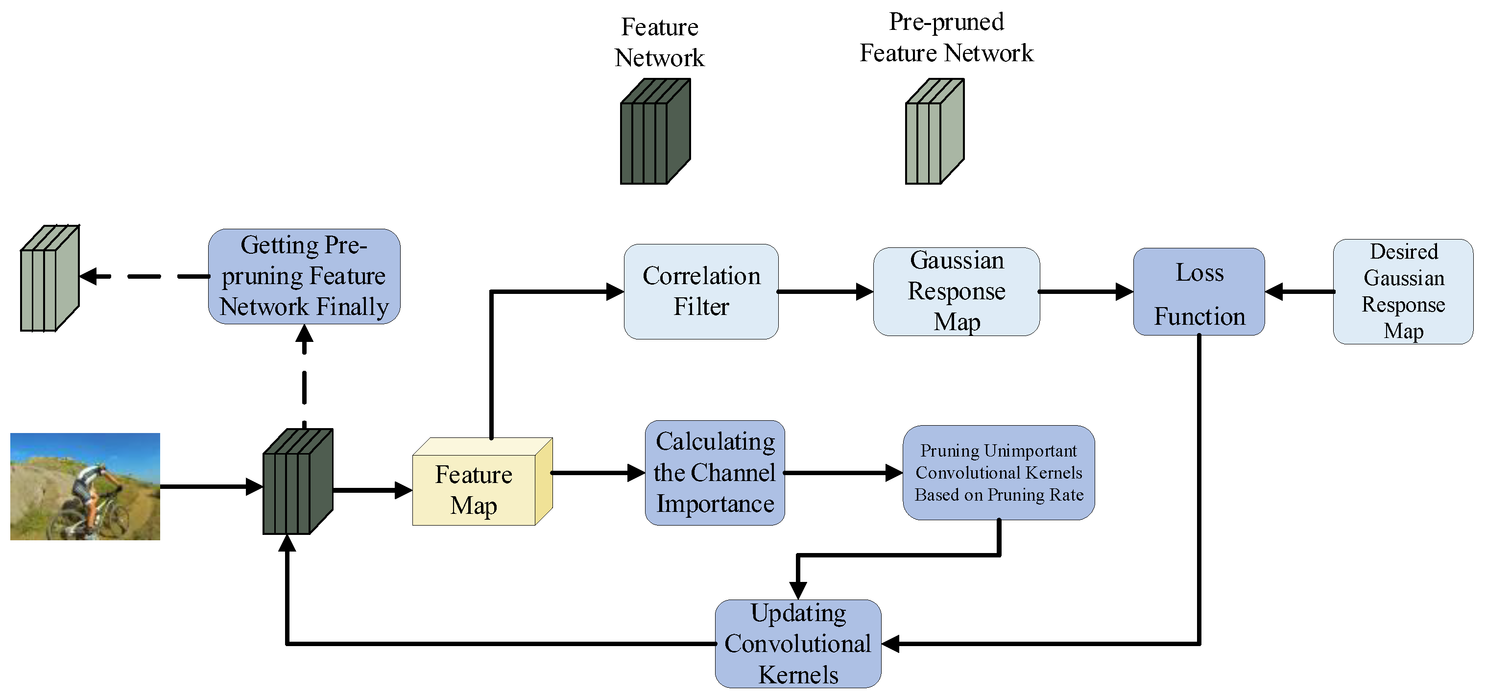
3.1. PCIP-Based Pre-Pruning of Deep Feature Network

It is assumed that the feature extraction network in the tracking model has $CL$ convolutional layers, the $ith\left(i\in \left(1,2,\dots ,CL\right)\right)$ convolutional layer has $CK{N}_i$ convolutional kernels, and the size of the convolutional kernels is $c{k}_i\times c{k}_i$ [30]. Following design policy, the feature network is pre-trained offline to provide effective deep features of the target for the downstream correlation filter tracking task. As shown in Figure 2, offline pre-training is accompanied by a pre-pruning of the feature network using the PCIP pruning algorithm [2]; then, the pre-pruned feature network is obtained.

Using $F_{i,j}$ to denote the feature map corresponding to the $jth$ convolutional kernel in the $ith$ convolutional layer, of which the size is $R_{i,j}\times C_{i,j}$, then the importance score $Scor{e}_{i,j}$ of the $jth$ convolutional kernel in the $ith$ convolutional layer can be derived from Equation (1) [2].

$$Scor{e}_{i,j}=Softmax\left(G_{i,j}\right)=\frac{e^{\frac{G_{i,j}}{T}}}{{{\displaystyle \sum }}^{\text{}}{e}^{\frac{G_{i,j}}{T}}}$$

(1)

where $G_{i,j}=\frac{1}{R_{i,j}\times C_{i,j}}{\displaystyle \sum }_{r=1}^{R_{i,j}}{\displaystyle \sum }_{c=1}^{C_{i,j}}{F}_{i,j}\left(r,c\right)$ and $T$ is the temperature parameter in the Softmax function. Based on the result of Equation (1), the convolutional kernels in layer i are reordered according to $Scor{e}_{i,j}$, $p_{i,j}$ denotes the reordered order of the $jth\left(j=1,2,\dots .,CK{N}_i\right)$ convolutional kernel in layer $i$. Assuming that the pruning rate in the pre-training stage is defined as $PR$, the convolutional kernels in layer i after reordering are divided into $CK{N}_i\ast PR$, significant convolutional kernels, and $CK{N}_i\ast \left(1-PR\right)$, unimportant convolutional kernels.

Set the $jth$ convolutional kernel in layer i to be $Kerne{l}_{ij}\left(k\right)$ at the $kth$ iteration; it is then iteratively updated according to Equations (2)–(4) [2]:

$$Kerne{l}_{ij}\left(k+1\right)=Kerne{l}_{ij}\left(k\right)+\eta {\nabla }_{Kerne{l}_{ij}}L\mathrm{oss}$$

(2)

$$Kerne{l}_{ij}\left(k+1\right)\ast {\beta }_{ij}\to Kerne{l}_{ij}\left(k+1\right)$$

(3)

$${\beta }_{ij}=\frac{1}{1+e^{\alpha \ast \left(p_{i,j}-CK{N}_i\ast PR\right)}}$$

(4)

where ${\beta }_{ij}$ denotes the penalty coefficient, which is used to moderately penalize the unimportant convolutional kernels, while the important convolutional kernels remain unchanged; $\alpha$ is used to regulate the trend of ${\beta }_{ij}$. When $\alpha$ is smaller, the trend of change is smoother, and vice versa, and steeper; Loss denotes the loss function of the whole model. ${\nabla }_{Kerne{l}_{ij}}L\mathrm{oss}$ is the gradient of the loss function in $Kerne{l}_{ij}\left(k\right)$.

The deep feature network is pruned while training offline and iteratively updated using Equations (1)–(4). After offline pre-training and pre-pruning, the pre-pruned feature network is obtained with $CL$ convolutional layers. Each convolutional layer has $PPCK{N}_i=CK{N}_i\ast PR$ convolutional kernels, all of which have the same size $c{k}_i\times c{k}_i$.

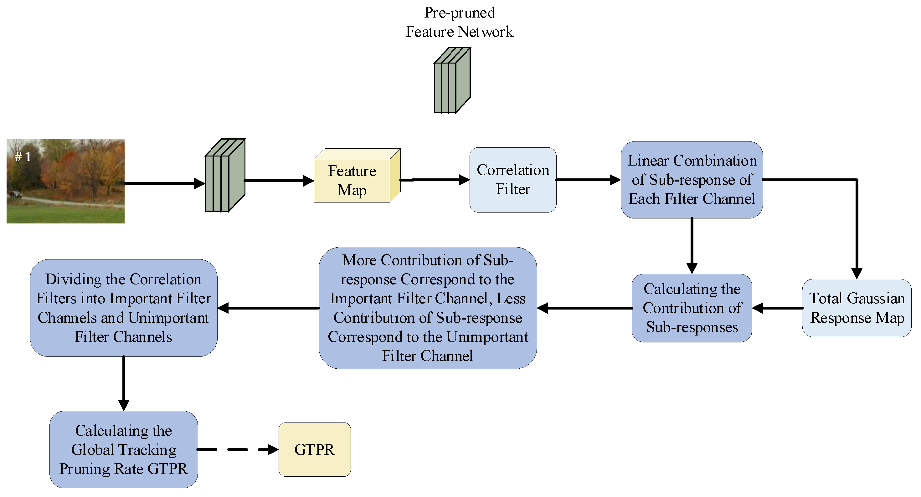
3.2. Optimal Determination of Global Tracking Pruning Rate Based on Tracking Response Contribution

As shown in Figure 3, the deep feature network is initially pruned to obtain a pre-pruned feature network with $PPCK{N}_{CL}$ convolutional kernels and corresponding $PPCK{N}_{CL}$ feature maps $F_{CL,l}$ (or feature channels), where $l=1,2,\dots ,PPCK{N}_{CL}$. The correlation tracking filter (which has $PPCK{N}_{CL}$ filter channels) is applied to $PPCK{N}_{CL}$ feature maps $F_{CL,l}$ and outputs $PPCK{N}_{CL}$ responses $g_l$ of size $M\times N$. The $PPCK{N}_{CL}$ responses are linearly overlapped to form the total response of the tracking model and the total response is approximated as a two-dimensional gaussian response [3]. The peak of the total response is the predicted position of the tracked target. Since the statistical distribution of each filter channel response and its peak point are different, the contribution of different filter channel responses to the total response of the tracked target is not the same.

It is assumed that $\left(x,y\right)$ denotes the peak point of the total 2-D gaussian response, i.e., the mean of the 2-D gaussian response, and ${\sigma }_{\mathrm{x}}$ and ${\sigma }_{\mathrm{y}}$ are the variances of the 2-D gaussian response. According to the properties of the 2-D gaussian distribution function, about 95.5% of the data are concentrated in a rectangular box centered at $\left(x,y\right)$ with a length of $2\times 2.58{\sigma }_{\mathrm{x}}$, and a width of $2\times 2.58{\sigma }_{\mathrm{y}}$ [3,31]. Since the total output response is a superposition of the responses of all single filter channels, the larger the proportion of single filter channel responses that fall within this rectangle, the greater the contribution of the filter channel to the total response is considered. The contribution $C{R}^l$ of a single filter channel $g_l$ can be obtained from Equations (5)–(7) [3]:

$$C{R}^l=\frac{rectanl{e}_{box}{}^l}{Whol{e}_{size}{}^l}$$

(5)

$$\begin{array}{c}rectanl{e}_{box}{}^l={\displaystyle \sum }_i{\displaystyle \sum }_j{ℱ}^{-1}\left(g_l\left(i,j\right)\right)\\ iϵ\left(\mathrm{x}-2.58{\sigma }_{\mathrm{x}},x+2.58{\sigma }_{\mathrm{x}}\right),jϵ\left(y-2.58{\sigma }_{\mathrm{y}},y+2.58{\sigma }_{\mathrm{y}}\right)\end{array}\}$$

(6)

$$Whol{e}_{size}{}^l={\displaystyle \sum }_{i=1}^M{\displaystyle \sum }_{j=1}^N{ℱ}^{-1}\left(g_l\left(i,j\right)\right)$$

(7)

where $\mathrm{M}\ge 2{\sigma }_x$, $\mathrm{N}\ge 2{\sigma }_y$; ${ℱ}^{-1}$ is the inverse Fourier transform; $rectanl{e}_{box}{}^l$ is the sum of the sample values of the output response of the filter channel $g_l$ that fall into the rectangular box, and $Whol{e}_{size}{}^l$ is the sum of all the sample values of the output response of the filter channel $g_l$,$l=1,2,\dots \dots ,PPCK{N}_{CL}$.

Based on $C{R}^l$, the $PPCK{N}_{CL}$ filter channels of the filter are sorted according to $C{R}^l$. For the sorted filter channels, a contribution ratio threshold (CRTH) is defined under the precondition that the tracking accuracy is satisfied. When $C{R}^l\ge CRTH$, the corresponding filter channel is retained (the number of retained filter channels is denoted by $RFC{N}_{CL}$ (remain feature channel number)). When $C{R}^l<CRTH$, the corresponding filter channel is removed (the number of removed filter channels is $PPCK{N}_{CL}-RFC{N}_{CL}$) to maximize the tracking speed.

Since the number of channels in the filter is equal to the number of channels in the last layer of the feature network, this also means that the number of channels that should be retained in the last layer of the feature network is represented by $RFC{N}_{CL}$, while the number of channels that should be removed is $PPCK{N}_{CL}-RFC{N}_{CL}$. Therefore, we define the global pruning rate of the feature network during the tracking process as ($GTPR$), which is expressed in Equation (8) as:

$$GTPR=\frac{RFC{N}_{CL}}{PPCK{N}_{CL}}$$

(8)

Then, for all the convolutional layers of the feature network, except the first layer, a secondary pruning is performed with the global tracking pruning rate, which further lightens the feature network and further improves the tracking speed.

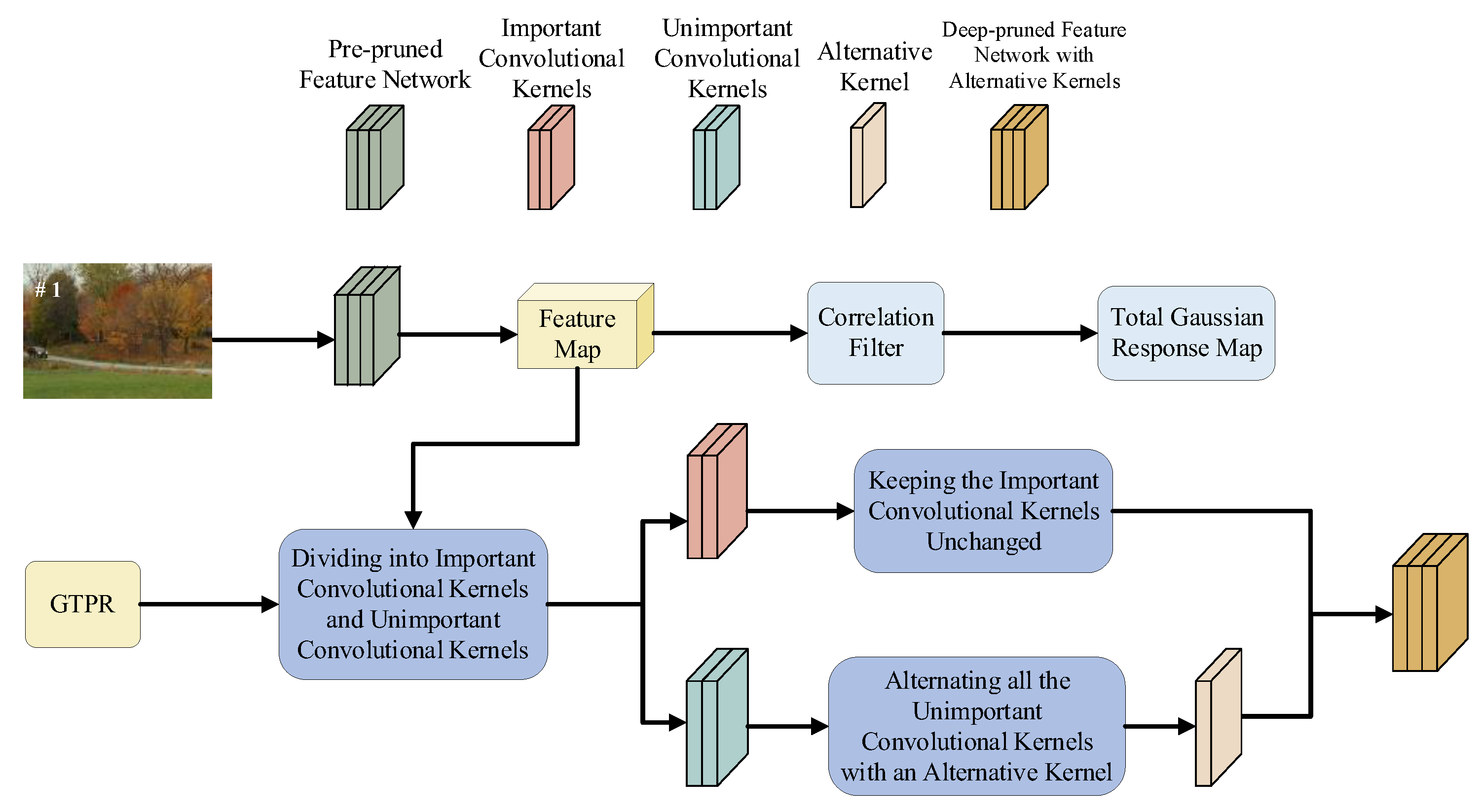
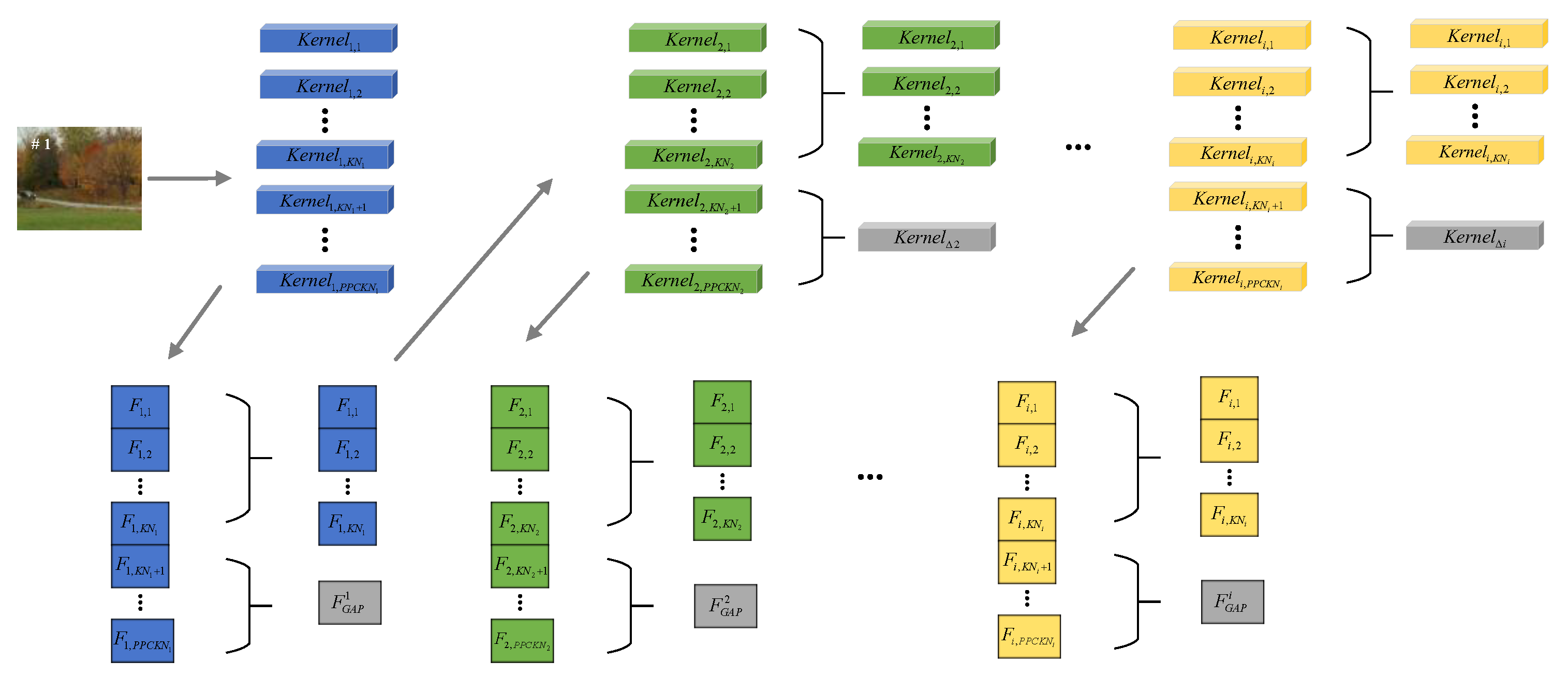
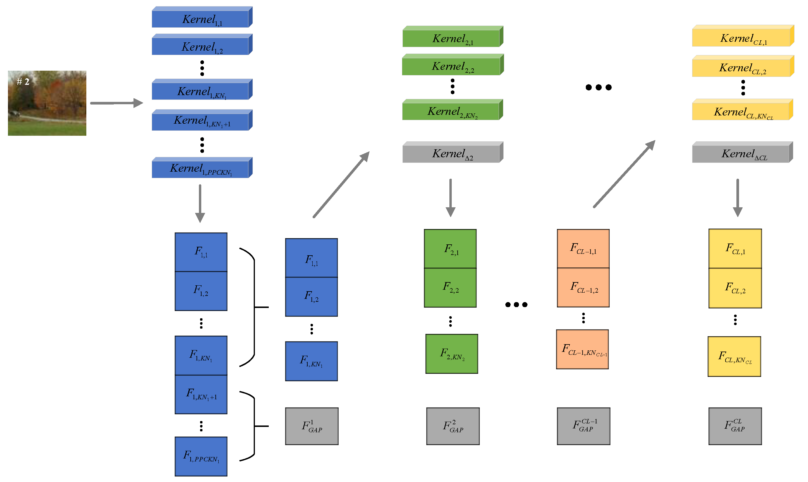
3.3. Secondary Pruning of Feature Extraction Network Based on Alternative Convolutional Kernels

The pre-pruned feature network obtained by pre-pruning is used as a feature extraction network for object tracking, which can achieve a certain degree of improvement in tracking speed while ensuring that the loss of accuracy does not affect the overall performance of the model. However, for the tracking system, there is a higher requirement for tracking speed enhancement. To accommodate this requirement, we consider a secondary pruning of the pre-pruned feature network before the start of the tracking process to further improve the tracking speed.

To further improve the tracking speed, we performed a secondary pruning on the feature network obtained from the pre-pruning in Section 3.1, based on the global tracking pruning rate ($GTPR$). If the pruning strategy of retaining $K{N}_i=PPCK{N}_i\times GTPR$ important convolutional kernels and removing $PPCK{N}_i\times 1-GTPR$ non-important convolutional kernels in each layer are directly adopted, the number of convolutional kernels in each layer and the complexity of the feature network can be reduced and improve the tracking speed. However, it is also very likely that removing too many convolutional kernels causes too significant a loss of accuracy in the feature network, which makes it difficult to accurately characterize the target and significantly degrades the tracking accuracy. To compensate for this deficiency, we introduce an alternative convolutional kernel that integrates the joint action of $PPCK{N}_i\times 1-GTPR$ unimportant convolutional kernels to each layer (except for the first layer, where the unimportant feature maps corresponding to the unimportant convolutional kernels in the first layer are used as the initial values for the iterative solutions of the alternative convolutional kernels in the subsequent layers) of the pre-pruned feature network, while retaining $K{N}_i=PPCK{N}_i\times GTPR$ important convolutional kernels. The alternative convolutional kernel is used to compensate for the loss of accuracy of the feature network caused by the removal of the $PPCK{N}_i\times (1-GTPR)$ unimportant convolutional kernels, which improves the feature network’s ability to characterize the tracked target, as shown in Figure 4. The iterative solution process for the alternative convolutional kernel in each layer is as follows.

The pre-pruned feature network is applied to the first frame of the tracking video sequence, as shown in Figure 5. $kerne{l}_{\mathsf{\Delta }i}$ is used to denote the operator of the combined action of $PPCK{N}_i-K{N}_i$ unimportant convolutional kernels ($kerne{l}_{i,(K{N}_i+1)},kerne{l}_{i,(K{N}_i+2)},\dots ,kerne{l}_{i,PPCK{N}_i}$) in the $ith$ convolutional layer, and it is called the alternative convolutional kernel of these $PPCK{N}_i-K{N}_i$ unimportant convolutional kernels. Let the feature maps corresponding to these $PPCK{N}_i-K{N}_i$ unimportant convolutional kernels be $F_{i,K{N}_i+1},F_{i,K{N}_i+2},\dots ,F_{i,PPCK{N}_i}$, then the global pooling $F_{GAP}^i$ corresponding to these $PPCK{N}_i-K{N}_i$ unimportant feature maps can be obtained from Equation (9).

$$\begin{array}{c}{F}_{GAP}^i=GAP\left({{\displaystyle \sum }}^{\text{}}{F}_{i,j}\right)\\ j\in \left(K{N}_i+1,K{N}_i+2,\dots ,PPCK{N}_i\right)\end{array}\}$$

(9)

Let the feature map corresponding to the alternative kernel $kerne{l}_{\mathsf{\Delta }i}$ of the $ith$ convolutional layer ($i\ne 1$) be $F_{\mathsf{\Delta }i}$, then:

$${\displaystyle \sum }_{j=1}^{PPKC{N}_{i-1}}Kerne{l}_{\mathsf{\Delta }i}\star F_{\left(i-1\right),j}=F_{\mathsf{\Delta }i}$$

(10)

where “⋆” denotes the convolution operation. Let $F_{\mathsf{\Delta }i}=F_{GAP}^i$, then the alternative convolutional kernel $kerne{l}_{\mathsf{\Delta }i}$ is initialized as:

$$kerne{l}_{\mathsf{\Delta }i}={ℱ}^{-1}\left(\frac{ℱ\left(F_{GAP}^i\right)}{ℱ\left({{\displaystyle \sum }}_{j=1}^{PPKC{N}_{i-1}}{F}_{\left(i-1\right),j}\right)}\right)$$

(11)

where “$ℱ$” denotes the Fourier transform and “${ℱ}^{-1}$” denotes the inverse Fourier transform.

After the secondary pruning operation and introducing the alternative kernel $kerne{l}_{\mathsf{\Delta }i}$ derived from Equations (10) and (11) into the pre-pruned feature network, the deep-pruned feature network with alternative kernels is obtained. The deep-pruned feature network with alternative kernels still has $CL$ convolutional layers, but each layer has $K{N}_i$ important convolutional kernels and one alternative kernel $kerne{l}_{\mathsf{\Delta }i}$. By using the deep-pruned feature network with alternative kernels as the feature network in the tracking system, on the one hand, the alternative kernel $kerne{l}_{\mathsf{\Delta }i}$ can effectively replace the multiple convolutional kernels removed in the secondary pruning process and compensate for the accuracy loss of the feature network caused by pruning; on the other hand, compared with the pre-pruned feature network, it further reduces the number of channels, decreases the computation, and improves the real-time performance of the tracking model.

3.4. Correlation Filter Tracking Model Based on the Deep-Pruned Feature Network

A deep-pruned convolutional neural network was obtained after a secondary pruning operation based on alternative kernels to maximize the tracking speed (at least the minimum requirement for practical applications, i.e., 25 FPS). The correlation filter tracking model based on the deep-pruned feature network is formed by cascading the deep-pruned feature network and the correlation filter. It mainly includes feature extraction, correlation filter initialization, target location prediction, correlation filter updating, and deep-pruned feature network updating, as shown in Figure 6. The details are described as follows.

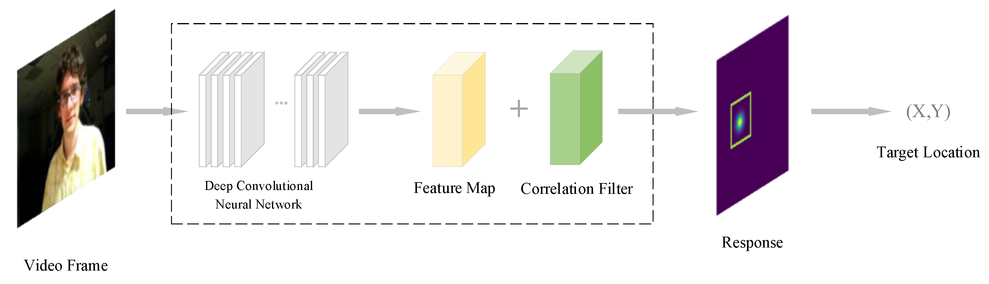
3.4.1. Feature Extraction

The deep-pruned feature network is applied to the second frame of the tracking video sequence, as shown in Figure 7.

From Figure 7, the first layer of the feature network has $PPCK{N}_1$ important convolutional kernels $kernel{1}_{1,1},kerne{l}_{1,2},\dots ,kerne{l}_{1,PPCK{N}_1}$, and the corresponding feature maps are $F_{1,1},F_{1,2},\dots ,F_{1,K{N}_1}{F}_{1,K{N}_1+1},F_{1,K{N}_1+2},\dots ,F_{1,PPCK{N}_1}$. Then, according to Equation (9), the global pooling $F_{GAP}^1$ corresponding to $PPCK{N}_1-K{N}_1$ unimportant feature maps in the first layer can be obtained as:

$$F_{GAP}^1=GAP\left({{\displaystyle \sum }}^{\text{}}{F}_{1,j}\right),j\in \left((K{N}_1+1,K{N}_1+2,\dots ,PPCK{N}_1\right)$$

(12)

Taking $F_{GAP}^1=F_{\mathsf{\Delta }1}$, then $F_{i,j}$ (where $i>1\mathrm{and}j\in \left(1,2,\dots ,K{N}_i\right)$) and $F_{\mathsf{\Delta }i}$ can be obtained from Equations (13) and (14):

$$\begin{array}{c}{\displaystyle {\displaystyle \sum }_{l=1}^{K{N}_{i-1}}}Kerne{l}_{i,j}\star F_{\left(i-1\right),l}+Kerne{l}_{i,j}\star F_{\mathsf{\Delta }\left(i-1\right)}=F_{i,j}\\ i\in \left(2,\dots ,CL\right),j\in \left(1,2,\dots ,K{N}_i\right)\end{array}\}$$

(13)

$$\begin{array}{c}{\displaystyle {\displaystyle \sum }_{l=1}^{K{N}_{i-1}}}Kerne{l}_{\mathsf{\Delta }i}\star F_{\left(i-1\right),l}+Kerne{l}_{\mathsf{\Delta }i}\star F_{\mathsf{\Delta }\left(i-1\right)}=F_{\mathsf{\Delta }i}\\ i\in \left(2,\dots ,CL\right)\end{array}\}$$

(14)

From Equations (13) and (14), the output feature map of the last layer of the deep-pruned feature network is $F_{CL,1},F_{CL,2},\dots ,F_{CL,K{N}_{CL}}$, which is the input of the correlation tracking filter.

3.4.2. Correlation Filter Initialization

Given an initial target box T in the second frame of the tracking video sequence, the corresponding ideal gaussian response $G$ is constructed based on the initial target box, and the peak point of the response corresponds to the position of the tracked target. The output feature maps of the last layer of the deep-pruned feature network are $F_{CL,1},F_{CL,2},\dots ,F_{CL,K{N}_{CL}}$, and the size of each feature map is M × N. Each feature map corresponds to one correlation filter channel. According to the literature [14,30,32,33,34], the correlation filter channel $W^l$ can be initialized by Equation (15) as:

$$W^l=\frac{\widehat{F_{CL,l}}\left(T\right)\odot {\widehat{G}}^{\ast }}{{{\displaystyle \sum }}_{k=1}^{K{N}_{CL}}\widehat{F_{CL,k}}\left(T\right)\odot {(\widehat{F_{CL,k}}\left(T\right))}^{\ast }+\lambda }\left(l=1,2,\dots K{N}_{CL}\right)$$

(15)

where $\odot$ refers to the Hadamard product, $\ast$ represents the complex conjugate, $\wedge$ represents the Fourier transform, $W^l$ represents the correlation filter channel corresponding to the $lth$ feature map channel, $\lambda$ is the regularization coefficient, and $\lambda \ge 0$.

3.4.3. Target Location Prediction

During the tracking process, a search box S of the same size as the initial target box T is constructed with the target location as the center. The deep-pruned feature network is used to extract the features of the area in which search box S is located and to record them as $F_{CL,l}\left(\mathrm{S}\right)\left(l=1,2,\dots ,K{N}_{CL}\right)$. Then the response ${\left(r_{i,j}\right)}_{M\times N}$ can be obtained from Equations (16) and (17) [30]:

$$g^l={\left({\widehat{W}}^l\right)}^{\ast }\odot {\mathrm{F}}_{CL,l}\left(S\right)\left(l=1,2,\dots K{N}_{CL}\right)$$

(16)

$${\left(r_{i,j}\right)}_{M\times N}={ℱ}^{-1}\left({\displaystyle \sum }_{l=1}^{K{N}_{CL}}{g}^l\right)$$

(17)

where, $g^l$ represents the frequency output response of the $lth$ tracking filter, ${ℱ}^{-1}$ represents the inverse Fourier transform, $r_{i,j}\in R^{M\times N}$ represents the total output response of all channels. Based on Equations (16) and (17), the coordinates $\left(x,y\right)$ of the predicted position of the target can be obtained as:

$$\left(x,y\right)=\underset{R^{M\times N}}{max}{\left(r_{i,j}\right)}_{M\times N}$$

(18)

3.4.4. Updating of Correlation Filter

In the tracking process, the position of the target in frame t is predicted to be $\left(x_t,y_t\right)$ based on the feature map $F_{CL,l}^{t-1}\left(S\right)\left(l=1,2,\dots ,K{N}_{CL}\right)$ of the target in frame $t-1$ using Equations (16)–(18). In frame $t$, a search box $S_t$ of the same size as the initial target box T is constructed centered on $\left(x_t,y_t\right)$, and the ideal gaussian response corresponding to this tracking box is $G_t\in R^{M\times N}$. The features of the region where $S_t$ is located are extracted using the deep-pruned feature network noted as $F_{CL,l}^t\left(S_t\right)$. The filter $W_t^l$ is updated online by Equation (19) [30].

$$W_t^l=\frac{{\widehat{F}}_{CL,l}^t\left(S_t\right)\odot {\left(\widehat{G_t}\right)}^{\ast }}{{{\displaystyle \sum }}_{k=1}^{K{N}_{CL}}{\widehat{F}}_{CL,k}^l\left(S_t\right)\odot {({\widehat{F}}_{CL,k}^t\left(S_t\right))}^{\ast }+\lambda }\left(l=1,2,\dots K{N}_{CL}\right)$$

(19)

Here, ${\widehat{F}}_{CL,l}^t\left(S_t\right)$ represents the Fourier transform of the $lth$ feature channel, and ${\left(\widehat{G_t}\right)}^{\ast }$ represents the complex conjugate of the Fourier transform of the ideal gaussian response $G_t$.

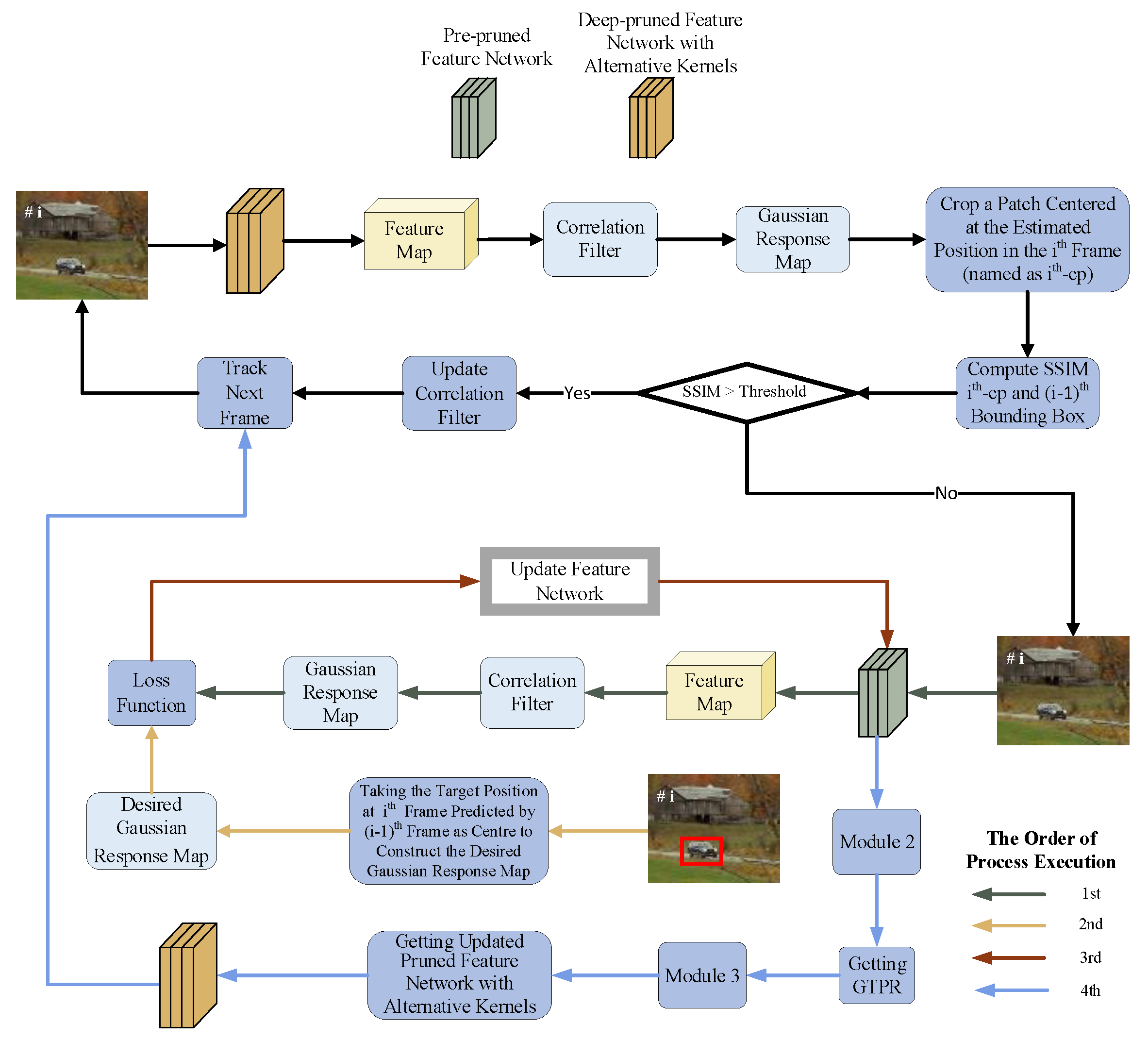
3.5. Online Updating of Deep-Pruned Feature Network with Alternative Kernels

In the actual tracking process, interference factors such as occlusion, illumination changes, target scaling, and background switching can affect the ability of the deep-pruned feature network to accurately characterize the tracked target features. This leads to target drift and tracking accuracy degradation. In severe cases, it can lead to tracking failure. To solve this problem, first, the adaptive capacity of the feature network is monitored in real-time during the tracking process. When the adaptive ability of the feature network is detected to decline, the feature network is updated online to improve its adaptive capacity to changes in the tracking scene.

SSIM [35] (structural similarity index) is a metric that measures the structural similarity of two images. It considers the blurred variation of structural information of images in human perception and measures the similarity of images in terms of brightness, contrast, and structure, respectively. SSIM has global statistical distribution characteristics, which are suitable for a wide range of interference factors and are also consistent with human visual habits. Therefore, we use SSIM as a measure to discriminate whether the adaptive ability of the feature network decreases during the tracking process.

To discriminate the adaptive ability of the feature network in the tracking process, the position of the target in frame $t-1$ is assumed to be $\left(x_{t-1},y_{t-1}\right)$, and the predicted position of the target in frame $t$ is $\left(x_t,y_t\right)$. The rectangular boxes $S_{t-1}$ and $S_t$ of the same size are the initial target boxes centered at $\left(x_{t-1},y_{t-1}\right)$ and $\left(x_t,y_t\right)$ constructed in frame $t-1$ and frame $t$, respectively. The SSIM of ${\mathrm{S}}_{t-1}$ and ${\mathrm{S}}_t$ is calculated using Equation (20) [35] as:

$$SSIM\left(S_{t-1},S_t\right)=\frac{\left(2{\mu }_{S_{t-1}}{\mu }_{S_t}+C_1\right)\left({\sigma }_{S_{t-1}{S}_t}+C_2\right)}{\left({\mu }_{S_{t-1}}^2+{\mu }_{S_t}^2+C_1\right)\left({\sigma }_{S_{t-1}}^2+{\sigma }_{S_t}^2+C_2\right)}$$

(20)

where ${\mu }_{{\mathrm{S}}_{t-1}}$ and ${\mu }_{{\mathrm{S}}_t}$ represent the means of $S_{t-1}$ and $S_t$, respectively. ${\sigma }_{S_{t-1}}$ and ${\sigma }_{S_t}$ represent the standard deviations of $S_{t-1}$ and $S_t$, respectively. ${\sigma }_{S_{t-1}{S}_t}$ represents the covariances of $S_{t-1}$ and $S_t$. $C_1$, $C_2$ are constants.

The similarity between $S_{t-1}$ and $S_t$ is judged based on the result of Equation (20) and the pre-defined target frame similarity threshold $TFSTH$. When SSIM is larger than $TFSTH$, $S_{t-1}$ and $S_t$ are considered similar, and the feature network has strong adaptability and does not need to be updated; when SSIM is less than $TFSTH$, it is considered that $S_{t-1}$ and $S_t$ are low in similarity, the adaptive capacity of the feature network decreases, and the feature network needs to be updated. The updating process of the feature network is as follows.

• Step 1. The desired gaussian response map, denoted as DGRM, is constructed by centering on the target location of the frame $tth$ predicted by frame $t-1th$, and the DGRM is used as Ground Truth.
• Step 2. The convolutional kernel parameters of the pre-pruned feature network are used as the initial values of the updating process, denoted as $Kerne{l}_{i,j}\left(t-1\right),\left(\mathrm{j}=1,2,\dots .,PPCK{N}_i\right)$.
• Step 3. Using the $tth$ frame as input, feature extraction is performed with the pre-pruned feature network, and the output features are correlated with the filter to generate the output response; i.e., Response. The error between Response and DGRM is calculated by the loss function defined in Equation (21), and the convolutional kernel parameters are updated once based on Equations (1)–(4). The $jth$ convolutional kernel in layer $i$ of the updated pre-pruned feature network is denoted as $Kerne{l}_{ij}\left(t\right)$.

  $$Loss={\Vert Response-DGRM\Vert }^2$$

  (21)
• Step 4. The $tth$ frame sequence is used as the input of the updated pre-pruned feature network, and the $GTPR$ is redetermined using Equations (5)–(8).
• Step 5. Based on the redetermined $GTPR$, the updated deep-pruned feature network with alternative kernels is obtained by updating the alternative convolutional kernels $kerne{l}_{\mathsf{\Delta }i}$ using Equations (9)–(11).
• Step 6. The updated deep-pruned feature network with alternative kernels is used as the new feature extraction network to continue tracking from the $t+1th$ frame sequence.

4. Experiment

4.1. Experiment Environment

To verify the effectiveness of the correlation filter tracking model based on the deep-pruned feature network proposed in this paper, the hardware and software experimental environment were designed and constructed. The hardware environment consisted of a terminal (AMD Ryzen 5 4600H), a server (X10DRG-Q), and a GTX 1080Ti graphics card (with a memory size of 12 GB). The software environment was as follows: Ubuntu 20.04 was selected as the operating system; Python was used for programming; and Pytorch based on deep learning was used as the development platform.

In this paper, we used the official VID dataset provided by the ILSVRC (ImageNet Large Scale Visual Recognition Challenge) competition 2015 [36] for feature network training and pre-pruning, and the OTB2013 [29] dataset for performance testing of the tracking model (including global pruning rate determination, secondary pruning, feature network updating, etc.).

4.2. Evaluation Metrics

In this paper, the OTB2013 dataset was used as the tracking dataset, so the curve evaluation method OPE (One-Pass Evaluation), which is common to the OTB dataset, was used in measuring the tracking performance of the model. OPE refers to initializing the first frame with the target location annotated in the dataset and then running the tracking algorithm to obtain the average accuracy and success rate. The OPE contains the average pixel error (APE) and the average overlap rate (AOR), which are the average of the precision rate and the success rate, respectively. Where the precision rate is the percentage of video frames where the distance between the center of the target box estimated by the tracking algorithm and the center of the target box manually labeled is less than a given threshold; the success rate is the percentage of video frames where the overlap rate (OR) between the predicted target box and the manually labeled target box obtained by the tracking algorithm is greater than a given threshold.

4.3. Experiment Design

To verify the effectiveness of the pruning strategy for improving tracking speed, and to verify whether the online updating algorithm can improve the model accuracy (APE and AOR), special experiments are designed, mainly including: (1) comparison experiments on tracking accuracy and speed of tracking models with or without pruning during the training process; (2) comparison experiments on accuracy and speed of tracking models of secondary pruned feature network and pre-pruned feature network; (3) comparison experiments on accuracy and speed of tracking models with or without adding alternative kernels; (4) comparison experiments on accuracy and speed of tracking models with or without online updating of feature network during tracking.

4.4. Experimental Results Analysis

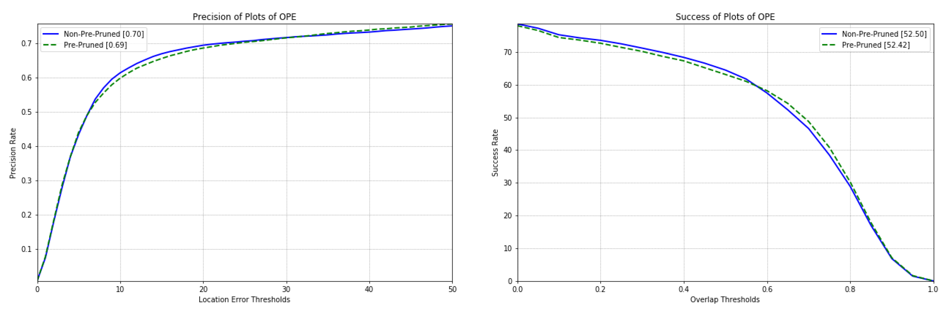
4.4.1. Comparative Study on Tracking Accuracy and Speed of Pre-Trained Feature Network before and after Pruning

In this paper, we designed the feature extraction network based on the DCFNet [30] tracking model. To simplify the design process and to illustrate our proposed pruning algorithm, the feature extraction network constructed in this paper has three convolutional layers, each layer with 32 convolutional kernels and a convolutional kernel size of 3 × 3. The constructed feature network is used as an un-pruned pre-trained feature network (non-pre-pruned feature network). The VID dataset is used as the pre-training dataset, the error sum of squares of the feature network output response and the desired gaussian response as the loss function. After 50 epochs of training, the non-pre-pruned feature network is obtained.

The same dataset and loss function are used, and the PCIP [2] algorithm is used to pre-train and prune the feature extraction network. In this pre-training process, the Temperature parameter T is set to 0.8 and the parameter α, which determines the trend of the penalty coefficient, is set to 10. After 50 epochs of pre-training and pruning, the pre-pruned feature network with three convolutional layers is obtained. Each convolutional layer has 26 convolutional kernels of size 3 × 3.

To verify the effectiveness of pre-pruning in improving the computational efficiency of the model, the tracking speed and tracking accuracy of the pre-trained feature network with pre-pruning are compared with those of the pre-trained feature network without pruning in the actual tracking process. Object tracking of video sequences in the OTB2013 dataset is performed using Formulas (15)–(19), and the results are shown in Figure 8 and

Table 1. AOR and APE, as well as speed of pre-pruned feature network or non-pre-pruned feature network, on the OTB2013 dataset.

Training Option	Non-Pre-Pruned	Pre-Pruned
AOR	52.50	52.42
APE	0.70	0.69
Speed	68.50	76.30

.

As shown in Figure 8 and Table 1, analyzing the tracking speed (FPS), tracking accuracy (average pixel error (APE)), and tracking success rate (average overlap rate (AOR)) can be seen. During the tracking process, although the APE of the pre-pruned feature network decreases by 0.01 and the AOR decreases by 0.08 compared to the non-pre-pruned feature network, the tracking speed increases by about 8 FPS. In practical object tracking applications, the relationship between tracking speed and tracking accuracy is contradictory, so it is common to increase the tracking speed as much as possible while ensuring tracking accuracy. Therefore, we use the PCIP algorithm to prune the feature network, which leads to a decrease in the tracking accuracy of the pre-pruned feature network, but still maintains 99% of the original model tracking accuracy level, and the improvement in tracking speed is of great significance for tasks such as object tracking that require high real-time performance.

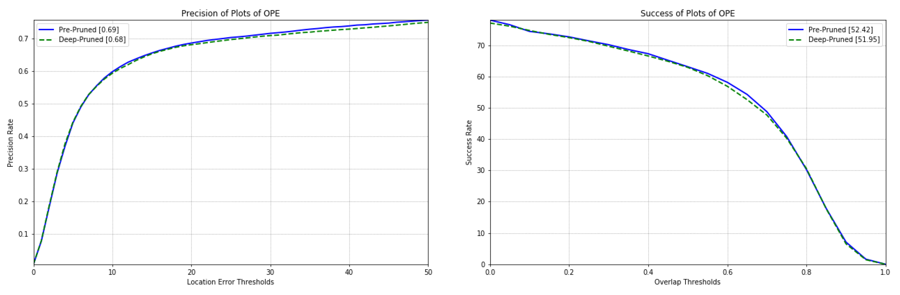
4.4.2. Comparative Study on Tracking Accuracy and Speed of Pre-Pruned Feature Network and Deep-Pruned Feature Network

The global pruning rate $GTPR$ is determined using the Formulas (5)–(8) before each video sequence in the OTB2013 dataset is tracked. The deep-pruned feature network is obtained by further pruning the pre-pruned feature network based on the global pruning rate $GTPR$, and its model size is further simplified. To evaluate the performance difference, based on Equations (15)–(19) and using the pre-pruned feature network and the deep-pruned feature network for object tracking of each video sequence in the OTB2013 dataset, respectively, the tracking results of both are shown in Figure 9 and

Table 2. AOR and APE, as well as speed of pre-pruned feature network or deep-pruned feature network, on the OTB2013 dataset.

Training Option	Pre-Pruned	Deep-Pruned
AOR	52.42	51.95
APE	0.69	0.68
Speed	76.30	99.50

.

From the tracking results shown in Figure 9 and Table 2, it can be seen that the APE of the tracker decreased by 0.01 and the AOR decreased by 0.47 for the deep-pruned feature network compared to the pre-pruned feature network, and the tracking speed improved by about 23 FPS. The performance difference mentioned above is due to the fact that the secondary pruning further compresses the network structure based on the initial pruning, which weakens the target characterization ability of the feature network and results in a decrease in the accuracy of the tracker. However, the advantage of the deep-pruned feature network is that it further reduces the computational load of the model and improves the speed of the tracker. Therefore, secondary pruning of the pre-pruned network results in a loss of accuracy of about 0.01, but in exchange for a speedup of almost 23 FPS. Thus, secondary pruning has a significant effect on further reducing the model size and increasing the tracking speed.

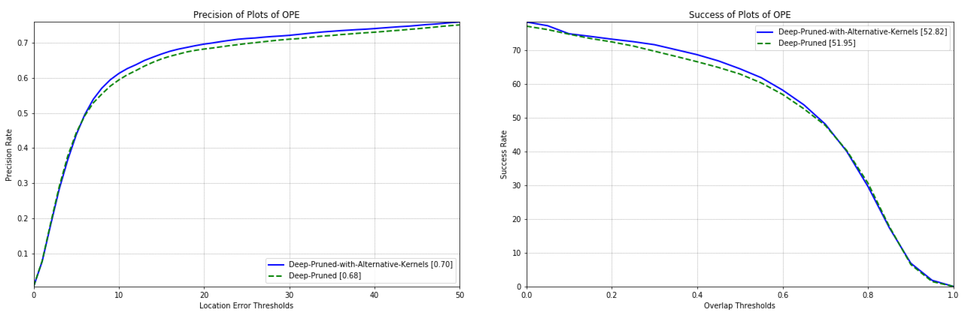
4.4.3. Comparative Study on Tracking Accuracy and Speed of Feature Network with or without Alternative Kernels

Considering that the target information and background information carried in different tracking video sequences may have large differences. To adapt the feature network to such differences, improve the robustness, and compensate for the accuracy loss of the feature network due to secondary pruning, based on Equations (9)–(11), we replace the multiple convolutional kernels with lower contributions that are removed from the corresponding convolutional layers with an alternative kernel in the secondary pruning process to obtain the deep-pruned feature network with alternative kernels. To measure the improvement of the feature network after the introduction of alternative kernels, based on Equations (15)–(19) and using the deep-pruned feature network with alternative kernels and deep-pruned feature network for object tracking of each video sequence in the OTB2013 dataset, respectively. The tracking results of both are shown in Figure 10 and

Table 3. AOR and APE, as well as speed of deep-pruned feature network or deep-pruned feature network with alternative kernels, on the OTB2013 dataset.

Training Option	Deep-Pruned	Deep-Pruned with Alternative Kernels
AOR	51.95	52.82
APE	0.68	0.70
Speed	99.50	97.60

.

From the tracking results shown in Figure 9 and Figure 10, and Table 2 and Table 3, it can be seen that the introduction of alternative kernels to the feature network leads to a decrease in tracking speed of about 2 FPS, which is about 21 FPS higher than that of the pre-pruned feature network, and about 29 FPS higher than that of the non-pre-pruned feature network. As for the tracking accuracy, the deep-pruned feature network with alternative kernels has a 0.02 improvement compared with the deep-pruned feature network, and can basically keep the same accuracy level as the non-pre-pruned feature network. Therefore, it can be concluded that the introduction of the alternative kernels can, on the one hand, maintain the performance improvement of the pruned feature network in terms of tracking speed; and on the other hand, it can improve the robustness of the feature network and effectively improve the accuracy loss caused by pruning.

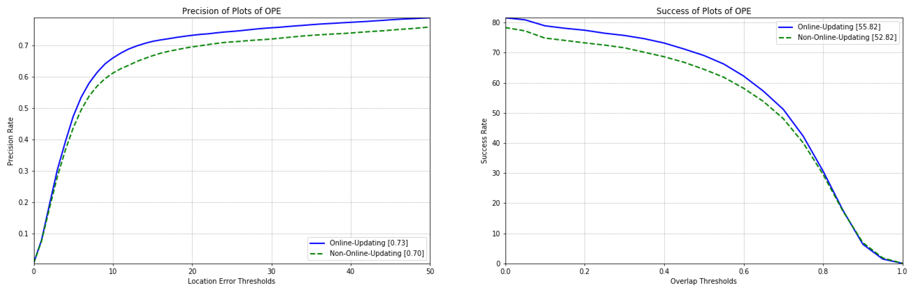
4.4.4. Comparative Study on Tracking Accuracy and Speed of Feature Network with or without Online Updating

In the actual tracking process, to monitor whether a large scene change has occurred in the current video sequence, we start from the second frame of the video sequence and use Equation (20) to calculate the SSIM of the current frame and the previous frame, and set the threshold value to 0.5. When SSIM is greater than the threshold value, it is considered that the current tracking scene has not significantly changed and there is no need to update the feature network; when SSIM is less than the threshold value, it is considered that at this time there has been a change in the scene that the feature network cannot adapt to, and it is necessary to update the feature network online using Equations (2), (5)–(11) and (21). Then use the updated feature network to continue the tracking process.

To verify whether online updating can improve the adaptability of the feature network to scene changes, the online updating operation was used as a control variable to measure the tracking performance of the deep-pruned feature network with alternative kernels, and the results are shown in Figure 11 and

Table 4. AOR and APE, as well as speed of online-updating or non-online-updating, on the OTB2013 dataset.

Training Option	Non-Online-Updating	Online-Updating
AOR	52.82	55.82
APE	0.70	0.73
Speed	97.60	84.80

.

As can be seen from the tracking results shown in Figure 11 and Table 4, the online updating for the feature network causes the speed of the tracker to be around 85 FPS, which is about 13 FPS lower compared to the non-online-updating strategy, but still about 16 FPS higher compared to the non-pre-pruned feature network. In terms of tracking accuracy, the tracking accuracy of the online updated feature network is 0.73, which is 0.03 higher than that of the non-pre-pruned feature network. The above results show that when the adaptability of the feature network to scene changes decreases, online updating can effectively improve its adaptability to scene changes while maintaining the improvement of tracking speed, thus improving the overall tracking performance of the tracker.

5. Discussion

To analyze the effectiveness of the pruning algorithm, the alternative convolution kernel, and the online updating algorithm more intuitively, the above experimental results are integrated as shown in

Table 5. Comparison of all experimental results.

Training Option	Non-Pre-Pruned	Pre-Pruned	Deep-Pruned	Deep-Pruned with Alternative Kernels	Online-Updating
AOR	52.50	52.42	51.95	52.82	55.82
APE	0.70	0.69	0.68	0.70	0.73
Speed	68.50	76.30	99.50	97.60	84.80

.

According to the results shown in the table, the tracking speed of the feature network without pruning operation is 68.5 FPS, while that of the feature network with deep pruning is 99.5 FPS, which is a 45% increase in speed. In terms of the tracking accuracy, the APE reaches 0.70 when alternative kernels are introduced into the feature network, which is the same level as the feature network before pruning. After further introducing the feature network online updating algorithm, the APE reaches 0.73, which is 4% higher than that of the deep-pruned feature network. Based on the above experimental results, the feature network pruning algorithm can simplify the network structure and effectively improve the tracking speed. The online updating algorithm can improve the adaptability of the feature network and increase the tracking accuracy when the tracking scene changes.

6. Conclusions

This paper proposes a correlation filter tracking model based on the deep-pruned feature network, which reduces the model complexity of the feature network and improves the tracking speed of the tracker while maintaining the object representation capability of the deep convolutional neural network and ensuring the tracking accuracy of the tracker when environment changes take place. Firstly, based on the pre-pruning network obtained by PCIP, an optimal global tracking pruning rate ($GTPR$) is determined in terms of the contribution of filter channels to tracking response. Secondly, based on ($GTPR$), an alternative convolutional kernel is defined to replace non-important channel kernels and maximally compensates for the accuracy loss of the feature network, which leads to the further pruning of the feature network. Thirdly, when large changes in the tracking scene are detected using the SSIM criterion during the actual tracking process, we adopt a strategy of online updating of the feature network, which effectively improves the adaptability of the feature network to changes in the tracking scene, and thus improves the tracking accuracy of the tracker. The experimental results based on the OTB2013 dataset illustrate the effectiveness of the proposed method in this paper. This paper provides an effective method for applying the deep correlation filter tracking model to real-world applications and deploying it to embedded and mobile devices with limited computational and memory resources. The implementation of this method on embedded mobile devices is the future major research work.

References

1. Li, C.; Chen, H. Research on lightweight deep correlation filter tracking algorithm based on fuzzy decision. In Proceedings of the 2021 2nd International Conference on Computer Science and Management Technology (ICCSMT), Shanghai, China, 12–14 November 2021; IEEE: Piscataway, NJ, USA, 2021. [Google Scholar]
2. Chen, H.; Li, C. Pruning deep feature networks using channel importance propagation. In Proceedings of the 2021 2nd International Conference on Computer Science and Management Technology (ICCSMT), Shanghai, China, 12–14 November 2021; IEEE: Piscataway, NJ, USA, 2021. [Google Scholar]
3. Yang, G.; Li, C.; Chen, H. Research on deep correlation filter tracking based on channel importance. EURASIP J. Adv. Signal Process 2022, 2022, 28. [Google Scholar] [CrossRef]
4. Li, C.; Yang, G. Deep correlation filter visual tracking algorithm based on channel importance and target similarity. (unpublished).
5. Comaniciu, D.; Meer, P. Mean shift: A robust approach toward feature space analysis. IEEE Trans. Pattern Anal. Mach. Intell. 2002, 24, 603–619. [Google Scholar] [CrossRef] [Green Version]
6. Shi, J. Good features to track. In Proceedings of the 1994 Proceedings of IEEE Conference on Computer Vision and Pattern Recognition, Seattle, WA, USA, 21–23 June 1994; IEEE: Piscataway, NJ, USA, 1994; pp. 593–600. [Google Scholar]
7. Nummiaro, K.; Koller-Meier, E.; Van Gool, L. An adaptive color-based particle filter. Image Vis. Comput. 2003, 21, 99–110. [Google Scholar] [CrossRef]
8. Bolme, D.S.; Beveridge, J.R.; Draper, B.A.; Lui, Y.M. Visual object tracking using adaptive correlation filters. In Proceedings of the 23rd IEEE Conference on Computer Vision and Pattern Recognition, CVPR 2010, San Francisco, CA, USA, 13–18 June 2010; IEEE: Piscataway, NJ, USA. [Google Scholar]
9. Henriques, J.F.; Caseiro, R.; Martins, P.; Batista, J. Exploiting the Circulant Structure of Tracking-by-Detection with Kernels. In Proceedings of the 12th European Conference on Computer Vision, Florence, Italy, 7–13 October 2012; Springer: Berlin/Heidelberg, Germany, 2012; Volume Part IV. [Google Scholar]
10. Henriques, J.F.; Rui, C.; Martins, P.; Batista, J. High-Speed Tracking with Kernelized Correlation Filters. IEEE Trans. Pattern Anal. Mach. Intell. 2015, 37, 583–596. [Google Scholar] [CrossRef] [PubMed] [Green Version]
11. Li, Y.; Zhu, J. A Scale Adaptive Kernel Correlation Filter Tracker with Feature Integration. In Proceedings of the Computer Vision–ECCV 2014 Workshops, Zurich, Switzerland, 6–12 September 2014; Agapito, L., Bronstein, M.M., Rother, C., Eds.; Springer International Publishing: Cham, Switzerland, 2015. [Google Scholar]
12. Krizhevsky, A.; Sutskever, I.; Hinton, G.E. Imagenet classification with deep convolutional neural networks. Commun. ACM 2017, 60, 84–90. [Google Scholar] [CrossRef] [Green Version]
13. Zhao, M.; Zhong, S.; Fu, X.; Tang, B.; Pecht, M. Deep residual shrinkage networks for fault diagnosis. IEEE Trans. Ind. Inform. 2019, 16, 4681–4690. [Google Scholar] [CrossRef]
14. Danelljan, M.; Häger, G.; Khan, F.; Felsberg, M. Accurate Scale Estimation for Robust Visual Tracking; Bmva Press: Blue Mountain, ON, Canada, 2014. [Google Scholar]
15. Xin, J.; Du, X.; Zhang, J. Deep learning for robust outdoor vehicle visual tracking. In Proceedings of the 2017 IEEE International Conference on Multimedia and Expo (ICME), Hong Kong, China, 10–14 July 2017; IEEE: Piscataway, NJ, USA, 2017. [Google Scholar]
16. Cheng, J.; Wang, P.; Li, G.; Hu, Q.; Lu, H. Recent advances in efficient computation of deep convolutional neural networks. Front. Inform. Technol. Elect. Eng. 2018, 19, 64–77. [Google Scholar] [CrossRef] [Green Version]
17. Li, P.; Wang, D.; Wang, L.; Lu, H. Deep visual tracking: Review and experimental comparison. Pattern Recognit. 2018, 76, 323–338. [Google Scholar] [CrossRef]
18. Voigtlaender, P.; Leibe, B. Online adaptation of convolutional neural networks for video object segmentation. arXiv 2017, arXiv:1706.09364. [Google Scholar]
19. Nam, H.; Han, B. Learning multi-domain convolutional neural networks for visual tracking. In Proceedings of the Computer Vision and Pattern Recognition (CVPR), Las Vegas, NV, USA, 27–30 June 2016; IEEE: Piscataway, NJ, USA, 2016. [Google Scholar]
20. Song, Y.; Ma, C.; Gong, L.; Zhang, J.; Lau, R.W.; Yang, M. Crest: Convolutional residual learning for visual tracking. In Proceedings of the IEEE International Conference on Computer Vision (ICCV), Venice, Italy, 2–29 October 2017; IEEE: Piscataway, NJ, USA, 2017. [Google Scholar]
21. Li, Y.; Song, L.; Chen, Y.; Li, Z.; Zhang, X.; Wang, X.; Sun, J. Learning dynamic routing for semantic segmentation. In Proceedings of the IEEE/CVF Conference on Computer Vision and Pattern Recognition (CVPR), Seattle, WA, USA, 13–19 June 2020; IEEE: Piscataway, NJ, USA, 2020. [Google Scholar]
22. Jia, X.; De Brabandere, B.; Tuytelaars, T.; Gool, L.V. Dynamic filter networks. In Proceedings of the Advances in Neural Information Processing Systems 29: Annual Conference on Neural Information Processing Systems 2016, Barcelona, Spain, 5–10 December 2016; p. 29. [Google Scholar]
23. Li, H.; Kadav, A.; Durdanovic, I.; Samet, H.; Graf, H.P. Pruning filters for efficient convnets. arXiv 2016, arXiv:1608.08710. [Google Scholar]
24. He, Y.; Kang, G.; Dong, X.; Fu, Y.; Yang, Y. Soft filter pruning for accelerating deep convolutional neural networks. arXiv 2018, arXiv:1808.06866. [Google Scholar]
25. Yang, X.; Lu, H.; Shuai, H.; Yuan, X.T. Pruning Convolutional Neural Networks via Stochastic Gradient Hard Thresholding. In Proceedings of the Second Chinese Conference, PRCV 2019, Xi’an, China, 8–11 November 2019; Springer: Berlin/Heidelberg, Germany, 2019; pp. 373–385. [Google Scholar]
26. Liu, Z.; Li, J.; Shen, Z.; Huang, G.; Yan, S.; Zhang, C. Learning efficient convolutional networks through network slimming. In Proceedings of the IEEE International Conference on Computer Vision, Venice, Italy, 2–29 October 2017; IEEE: Piscataway, NJ, USA, 2017. [Google Scholar]
27. Ye, Y.; You, G.; Fwu, J.; Zhu, X.; Yang, Q.; Zhu, Y. Channel pruning via optimal thresholding. In Proceedings of the 27th International Conference, ICONIP 2020, Bangkok, Thailand, 18–22 November 2020; Springer: Berlin/Heidelberg, Germany, 2020. [Google Scholar]
28. Zhuling, Q.; Yufei, Z.; Peng, Z.; Min, W. Visual Tracking Algorithm Based on Online Feature Discrimination with Siamese Network. Acta Opt. Sin. 2019, 39, 915003. [Google Scholar] [CrossRef]
29. Wu, Y.; Lim, J.; Yang, M. Online object tracking: A benchmark. In Proceedings of the 2013 IEEE Conference on Computer Vision and Pattern Recognition, Portland, OR, USA, 23–28 June 2013; IEEE: Piscataway, NJ, USA, 2013. [Google Scholar]
30. Wang, Q.; Gao, J.; Xing, J.; Zhang, M.; Hu, W. Dcfnet: Discriminant correlation filters network for visual tracking. arXiv 2017, arXiv:1704.04057. [Google Scholar]
31. Curran-Everett, D.; Taylor, S.; Kafadar, K. Fundamental concepts in statistics: Elucidation and illustration. J. Appl. Physiol. 1998, 85, 775–786. [Google Scholar] [CrossRef] [PubMed]
32. Danelljan, M.; Hager, G.; Shahbaz Khan, F.; Felsberg, M. Learning spatially regularized correlation filters for visual tracking. In Proceedings of the 2015 IEEE International Conference on Computer Vision (ICCV), Santiago, Chile, 7–13 December 2015; IEEE: Piscataway, NJ, USA, 2015. [Google Scholar]
33. Danelljan, M.; Robinson, A.; Shahbaz Khan, F.; Felsberg, M. Beyond correlation filters: Learning continuous convolution operators for visual tracking. In Proceedings of the 4th European Conference, Amsterdam, The Netherlands, 11–14 October 2016; Springer: Berlin/Heidelberg, Germany, 2016. [Google Scholar]
34. Danelljan, M.; Bhat, G.; Shahbaz Khan, F.; Felsberg, M. Eco: Efficient convolution operators for tracking. In Proceedings of the Conference on Computer Vision and Pattern Recognition (CVPR), Honolulu, HI, USA, 21–26 July 2017; IEEE: Piscataway, NJ, USA, 2017. [Google Scholar]
35. Wang, Z.; Bovik, A.C.; Sheikh, H.R.; Simoncelli, E.P. Image quality assessment: From error visibility to structural similarity. IEEE Trans. Image Process. 2004, 13, 600–612. [Google Scholar] [CrossRef] [PubMed] [Green Version]
36. Russakovsky, O.; Deng, J.; Su, H.; Krause, J.; Satheesh, S.; Ma, S.; Huang, Z.; Karpathy, A.; Khosla, A.; Bernstein, M. Imagenet large scale visual recognition challenge. Int. J. Comput. Vis. 2015, 115, 211–252. [Google Scholar] [CrossRef]
Figure 1. The general process of deep correlation filter tracking model.
Applsci 12 11490 g001
Figure 2. PCIP-based pre-pruning of the deep convolutional feature network.
Applsci 12 11490 g002
Figure 3. Optimal determination of global tracking pruning rate based on tracking response contribution. ( # i indicates the i t h picture in the video sequence).
Applsci 12 11490 g003
Figure 4. Definition and initialization of alternative convolutional kernels, and secondary pruning of deep feature extraction network. ( # i indicates the i t h picture in the video sequence).
Applsci 12 11490 g004
Figure 5. Initialization of the alternative kernels by applying the pre-pruned feature network to the first frame of the tracking video sequence. ( # i indicates the i t h picture in the video sequence).
Applsci 12 11490 g005
Figure 6. Correlation filter tracking model based on the deep-pruned feature network and online updating process of the deep-pruned feature network (including alternative kernels). ( # i indicates the i t h picture in the video sequence).
Applsci 12 11490 g006
Figure 7. The deep-pruned feature network is applied to the second frame of the tracking video sequence for feature extraction. ( # i indicates the i t h picture in the video sequence).
Applsci 12 11490 g007
Figure 8. Success and precision plots on OTB2013 dataset with pre-pruned feature network or non-pre-pruned feature network.
Applsci 12 11490 g008
Figure 9. Success and precision plots on OTB2013 dataset with pre-pruned feature network or deep-pruned feature network.
Applsci 12 11490 g009
Figure 10. Success and precision plots on OTB2013 dataset with deep-pruned feature network or deep-pruned feature network with alternative kernels.
Applsci 12 11490 g010
Figure 11. Success and precision plots on OTB2013 dataset with online-updating or non-online-updating.
Applsci 12 11490 g011