Review

Review of Quantitative Methods for the Detection of Alzheimer’s Disease with Positron Emission Tomography

1
Graduate Program in Biomedical Engineering, Price Faculty of Engineering, University of Manitoba, Winnipeg, MB R3T 2N2, Canada
2
Health Sciences Centre, Kleysen Institute for Advanced Medicine, Winnipeg, MB R3E 3J7, Canada
3
Department of Human Anatomy and Cell Science, Max Rady College of Medicine, Rady Faculty of Health Sciences, University of Manitoba, Winnipeg, MB R3E 0W2, Canada
*
Author to whom correspondence should be addressed.
Appl. Sci. 2022, 12(22), 11463; https://doi.org/10.3390/app122211463
Submission received: 2 October 2022 / Revised: 29 October 2022 / Accepted: 3 November 2022 / Published: 11 November 2022
(This article belongs to the Special Issue Deep Learning and Machine Learning in Biomedical Data)

Abstract

:

Featured Application

A thorough review of the quantitative methods for the detection of Alzheimer’s from neuroimaging studies acquired with positron emission tomography, with a special emphasis on supervised machine/deep learning techniques for specialist physicians, neuroscientists, computer scientists, and other allied professions in dementia care and diagnosis.

Abstract

The dementia spectrum is a broad range of disorders with complex diagnosis, pathophysiology, and a limited set of treatment options, where the most common variety is Alzheimer’s disease (AD). Positron emission tomography (PET) has become a valuable tool for the detection of AD; however, following the results of post-mortem studies, AD diagnosis has modest sensitivity and specificity at best. It remains common practice that readings of these images are performed by a physician’s subjective impressions of the spatial pattern of tracer uptake, and so quantitative methods based on established biomarkers have had little penetration into clinical practice. The present study is a review of the data-driven methods available for molecular neuroimaging studies (fluorodeoxyglucose-/amyloid-/tau-PET), with emphasis on the use of machine/deep learning as quantitative tools complementing the specialist in detecting AD. This work is divided into two broad parts. The first covers the epidemiology and pathology of AD, followed by a review of the role of PET imaging and tracers for AD detection. The second presents quantitative methods used in the literature for detecting AD, including the general linear model and statistical parametric mapping, 3D stereotactic surface projection, principal component analysis, scaled subprofile modeling, support vector machines, and neural networks.

1. Introduction

Under the paradigm of early detection and intervention, disease-modifying therapies and preventative strategies are most effective when used as early as possible in the progression of Alzheimer’s disease (AD). Current clinical practice uses medical history and neuropsychological examination as the primary means of establishing a diagnosis of dementia [1]. A diagnosis of dementia does allow access to specialized care and therapies; however, a diagnosis at the stage where serious cognitive symptoms have become clinically evaluable does not allow for the full effect of disease-modifying therapies which delay or reduce cognitive symptoms. Diagnostic accuracy at this stage has also been revealed as modestly sensitivity-specific at best due to the overlapping clinical presentation of multiple forms of dementia spectrum disorders (DSDs), as confirmed by large post-mortem studies across multiple laboratories [2,3,4]. The potentially prodromal state of mild cognitive impairment (MCI) further complicates the diagnostic task because approximately 20% of all MCI patients progress to develop some form of dementia with 3–5 years of diagnosis (pMCI), while the balance will remain stable and see a plateau in their cognitive decline (sMCI) [5,6].
Distinct alterations in the basal rates of glucose metabolism have been found to precede and coincide with the clinical manifestation of dementia-related cognitive symptoms [5,6,7,8]. Patients suspected of having AD may undergo brain positron emission tomography (PET) imaging with a variety of tracers; however, these images are commonly evaluated by a physician’s subjective impression of tracer uptake instead of being subject to quantitative analysis. Data-driven neuroimaging has great potential to alleviate the issue of diagnostic inaccuracy and increase confidence in clinical decision-making by providing objective quantitative metrics to complement the specialist physician, but thus far it has seen limited application in clinical practice [9,10,11].
This article presents a detailed review of the use of data-driven methods to detect AD neuropathology from several varieties of PET neuroimaging studies, with an emphasis on the application of machine/deep learning methods to complement clinical evaluation. We first present an overview of AD’s epidemiology, pathology, and the most widely recognized biomarkers. Next, we survey several PET tracers that are useful for the detection of AD in the context of AD as a progressive proteinopathic disorder. Finally, we detail the quantitative methods useful for detecting AD from PET studies and survey the representative literature for each of these methods.

2. Alzheimer’s Disease—Epidemiology, Progression, ATN Biomarkers

Alzheimer’s disease (AD) is an age-related chronic illness characterized by progressive global deterioration in learning, memory, communication, and general cognitive functioning. AD is the most common cause of dementia spectrum disorder (DSD) and accounts for nearly two-thirds of all dementia diagnoses worldwide [12]. Currently, there are approximately 26 million people worldwide living with AD-derived dementia, and this number is expected to increase dramatically to over 100 million by the mid-century, or an estimated prevalence of 324 per 10,000 persons, and an annual cost of care in the hundreds of billions of dollars worldwide [12,13]. AD patients are likely to require extensive personal care for the remainder of their lives due to their cognitive impairment [14]. There is no effective treatment or cure for AD, and the continued neurodegeneration is ultimately fatal to the patient. The available treatment options focus on slowing down the progression and the severity of the symptoms of AD. Some preventative measures have also been identified, such as the maintenance of a cognitive reserve or the elimination of behavioral risk factors [14]. Other non-preventable risk factors, such as genetics, have also been identified. Pharmaceutical support does exist in the form of acetylcholinesterase inhibitors [15]. The recent development and accelerated FDA approval of amyloid beta-targeting drugs such as aducanumab have raised hopes; however, their uses are limited, and their efficacy remains controversial [16,17].
AD is histopathologically characterized by abnormal accumulations of protein on the brain or altered protein content in cerebrospinal fluid (CSF). Well-known examples include an increase in extracellular amyloid plaques (also known as senile plaques) on the brain and decreased amyloid protein levels found in CSF; the appearance of intracellular neurofibrillary tangles composed of hyperphosphorylated tau proteins; and decreased total tau protein levels in CSF. The accumulation of these is followed by generalized neurodegeneration and cognitive decline [6,18]. Single-cell transcriptome analysis reveals that there are multiple genes that are involved in the development of AD, most notably those that affect the ability of microglia to clear amyloid proteins from the brain or that affect the regulation of astrocytes [19]. It must be noted that the exact etiology of AD is currently unknown, and that many different factors (synaptic, mitochondrial, inflammatory, neuronal, cytoskeletal, vascular, age, lifestyle, demographic, and genetic) are likely to play mutually overlapping roles in the progression of AD.
Jack et al., have proposed the now commonly known amyloid-tau-neurodegenerative (ATN) biomarker-based staging framework, which incorporates the most widely recognized clinical biomarkers of AD [18]. The ATN framework is a descriptive system for communicating multimodal biomarkers for a patient suspected of having AD. Status is reported in a binary fashion (positive or negative) to support the ease of use, clarity, and portability between medical domains. Amyloid positivity is supported by either significant ligand retention in amyloid-PET or low amyloid levels in CSF. Tau positivity is similarly supported by high ligand retention in tau-PET or else elevated levels of phosphorylated tau proteins in CSF. Neurodegeneration (or neuronal injury) is supported by elevated total tau protein levels in CSF, hypometabolism in fluorodeoxyglucose positron emission tomography (FDG-PET), or atrophy in specific brain regions revealed by structural magnetic resonance (MR) images [18]. It is important to note that while extracellular amyloid plaques and intracellular neurofibrillary tangles of hyperphosphorylated tau proteins are not causal factors in AD pathogenesis, AD is characterized along a biologically progressive spectrum by the abnormal accumulation of these specific proteins. In combination with neurodegeneration, they form the primary diagnostic markers [18]. The ATN model is also very amenable to extension should further important biomarkers be discovered in the future. This biomarker-based framework for AD detection has informed the emphasis of this review on FDG, amyloid, and tau tracers.

3. Positron Emission Tomography & Tracers for the Detection of AD

Positron emission tomography (PET) has become an important clinical tool for non-invasive in vivo characterization, visualization, and measurement of physiological processes. The success of PET imaging is due to the development of radiopharmaceuticals called tracers, which are radiolabeled molecules administered in sub-pharmacological dosages for the purpose of performing nuclear imaging procedures. The development and clinical evaluation of tracers for neuroimaging is a highly active field of research and continues to grow in parallel with advances in neurochemistry and the pathology of neurological disorders [19,20,21,22,23,24,25]. Tracer design for neuroimaging is a complex process that must account for many factors, the most prominent of which are the ability to cross the blood-brain barrier (BBB), ligand specificity, ligand metabolism, non-specific binding, and the effect of unbound ligands on normal physiology [22]. The guiding principle of tracer-based imaging is that the distribution and concentration of a tracer are an indication of the regionalized abundances of the target for which the tracer is designed. For the purposes of the current work, we will survey three groups of PET tracers relevant to the in vivo detection of AD: fluorodeoxyglucose (FDG), amyloid-binding tracers, and tau-binding tracers. While there are many other PET tracers in existence that may be used to investigate AD pathology (e.g., cholinergic tracers, inflammatory tracers, 15O-based imaging), only the use of FDG is considered the current clinical norm; however, the use of amyloid and tau tracers is rapidly becoming more common [26,27,28,29]. For each, we present the histological/pathological evidence for the use of these tracers and then common themes of research resulting from their use.

3.1. Fluorodeoxyglucose (FDG)

FDG (2-[18F]-fluoro-2-deoxy-D-glucose) is a glucose analog that does not undergo glycolysis and hence accumulates in the brain at the same rate that glucose would be metabolized. FDG has been routinely used for decades to monitor brain glucose metabolism as a reliable proxy of synaptic activity [30]. It is well known that changes in FDG uptake precede the structural atrophy in neurodegenerative disorders that may be visualized by MR or CT imaging [31,32]. AD patients exhibit progressive and usually bilateral glucose hypometabolism compared to healthy controls. As seen in Figure 1, this occurs specifically within the parietal and temporal cortices, but also in the frontal and posterior cingulate cortices and the precunei. Metabolism is mostly preserved in the primary sensorimotor cortex, basal ganglia, thalamus, brainstem, and primary visual cortex. The degree and size of the area of distribution of hypometabolism also correlate with the estimated severity of AD dementia and decreased scores on clinical tests of cognitive function. MCI patients also show heterogeneous patterns of hypometabolism throughout the brain, in keeping with the fact that MCI patients may eventually develop non-AD dementias, though most MCI patients show hypometabolism in the medial temporal cortex; however, this is also a common finding in elderly healthy controls [20,32]. Hypometabolism within the posterior cingulate cortex, inferior parietal lobe, and precunei is common in prodromal AD patients. Progressive parietotemporal hypometabolism is also found in asymptomatic carriers of the allele APOE-ε4, a gene that significantly increases the lifetime risk of developing AD [33]. Because glucose metabolism is spared in the posterior cingulate cortex and the precunei in non-AD DSDs, FDG-PET is also useful in their differential diagnosis [34]. FDG-PET has also been used for monitoring outcomes in many AD therapeutics, specifically by tracking changes in regionalized or global tracer uptake [35,36,37,38].

3.2. Amyloid-Binding Tracers

The development of the amyloid cascade hypothesis highlights the role of a range of dynamic and heterogeneous soluble amyloid species as the primary instigator of neurotoxicity and cellular dysfunction [40]. Both synthetic and proto-fibrillar amyloid species have been demonstrated to directly induce oxidative stress, neuroinflammation, and synaptic hyperactivity, leading to neurodegeneration and the development of several amyloid-binding tracers and clinical trials of amyloid-targeting pharmaceuticals [41,42,43]. AD patients also display higher cortical retention of amyloid than elderly healthy controls in the orbitofrontal, inferior parietal/posterior cingulate cortices, and the precunei [44]. Cortical retention of amyloids also appears to stop increasing upon reaching a plateau early on in disease progression; however, there is some evidence to suggest this may not be a universal feature of amyloid accumulation [45].
The first amyloid tracer was N-methyl-[11C]-2-(4-methylaminophenyl)-6-hydroxybenzothiazole, which is commonly known as Pittsburgh compound B or PIB and is a derivative of the amyloid staining compound thioflavin-T [46,47]. It has been shown that the distribution and retention of PIB in vivo correlate very well with amyloid found post-mortem at autopsy and shows that PIB is sensitive to soluble and insoluble forms of amyloid protein [48]. Amyloid imaging with PIB is also sensitive in differentiating AD patients from elderly healthy controls; however, imaging studies in MCI patients have revealed a bimodal distribution of amyloid positivity. However, those with a greater amyloid burden are more likely to develop AD [49,50,51]. The retention of PIB also correlates with glucose hypometabolism in the parietotemporal regions in AD patients but not in those with MCI [47,52]. As with FDG-based imaging, carriers of the APOE-ε4 allele show a greater degree of amyloid plaque deposition revealed by PIB imaging [46].
The greatest challenge to the clinical adoption of PIB has been the short half-life of the 11C atom at approximately 20 min, which has greatly limited its use to locales with an on-site cyclotron. This has driven the development of 18F-based tracers for amyloid imaging since the half-life is much longer at nearly two hours. This not only greatly increases ease-of-access but also yields less noisy images, which allows for more precise quantitation. Three of these fluorine-based tracers have received approval for clinical use (tradenames: florbetapir, florbetaben, and flutemetamol), and these have been demonstrated to correlate well with the results of PIB studies and post-mortem autopsies [53,54]. Differences in target sensitivity and non-specific binding between these have been reported; however, efforts are underway to standardize amyloid staging, such as the centiloid project [55].
Amyloid-based imaging is not without its drawbacks. Amyloid is extremely useful for the differential diagnosis of DSDs that do not have an amyloid pathology, such as frontotemporal dementia disorder (FTD); however, the presence of accumulated extracellular amyloid plaques is relatively common in the general population of older adults [55,56]. As such, it is a nonspecific indicator on its own, so its diagnostic value is as a predictor of possible future effects, or else it must be considered in conjunction with other more specific biomarkers.

3.3. Tau-Binding Tracers

The accumulation of neurofibrillary tangles of hyperphosphorylated tau proteins is a well-known pathological characteristic of AD alongside the accrual of amyloid plaques [57]. The amyloid cascade hypothesis states that downstream from the accumulation of insoluble amyloid, misfolded and hyperphosphorylated tau proteins weaken tau’s binding affinity to microtubules within neuronal bodies, resulting in the generalized breakdown of cytoskeletal architecture and leading to neurodegeneration [58]. Tau deposition in vivo correlates very well with hypometabolism revealed by FDG-PET and also with Braak staging in post-mortem studies. Tau retention tends to first occur in the hippocampus and entorhinal cortex during Braak stages I–II, adjacent neocortices in Braak stages III–IV, and throughout the whole brain in Braak stages V–VI [20,59,60]. The accumulation of tau tangles in the temporal lobe is inversely correlated with memory performance, while accumulation in the frontal lobe is inversely correlated with general cognition, and with FDG-PET and amyloid-PET [61,62]. Individuals with the APOE-ε4 allele showed a substantially increased tau protein burden [63,64].
The development of tracers for tau-PET has been marked by significant challenges regarding off-target binding, specifically to amyloid proteins and monoamine oxidase [65]. Even highly tau-specific tracers must deal with the complication of tau proteins having many unique isoforms with significantly different structures at the secondary and tertiary levels of protein organization, making isoform selectivity an important challenge to overcome [66]. Tau tracer design is further complicated by the fact that neurofibrillary tau tangles occur within neuronal bodies, which would require that the tracer not only be capable of crossing the BBB but also be capable of crossing neuronal cell membranes. Currently, there is only one tracer that is approved for clinical use by the FDA (tradename: flortaucipir); however, extensive effort is underway to design validation procedures for the design of next-generation tau tracers [67,68,69,70].
One important advantage of tau-PET over amyloid-PET is that tau neurofibrillary tangles follow a well-defined sequential spread defined by Braak stages, which is markedly different from the plateau typically seen in amyloid accumulation. The spread of these tau tangles may, in fact, be indicative of disease progression in vivo [57,59]. Tau-PET has been shown to outperform amyloid-PET and volumetric MR studies for the prognostication of cognitive decline [71]. As with the accumulation of amyloid plaques, the presence of tau tangles does not necessarily prescribe a diagnosis of AD dementia nor any other DSD. For instance, tau deposition also occurs in elderly healthy control patients in a process known as primary age-related tauopathy (PART) and is believed to be an insufficient condition for the progression of cognitive decline in the absence of amyloid positivity [72]. Tau-PET may also be very useful in the differential diagnosis of non-tauopathic DSDs (e.g., Parkinson’s disease dementia and multiple system atrophy).

4. Quantitative Methods for the Detection of AD

In current clinical practice, both the patient’s medical history and the physician’s neuropsychological examination are the primary means of establishing a diagnosis of dementia; however, clinical diagnosis comes very late in AD progression [1]. Beach et al., discovered that the diagnosis of AD by specialist physicians in living patients is at best modestly sensitive (70.9–87.3%) and generally nonspecific (44.3–70.8%) over a wide range of clinical diagnostic criteria. Diagnostic accuracy was found to be particularly poor in the cases of mild early AD progression [2]. Even post-mortem autopsy-based diagnosis can vary across laboratories due to significant variations in interobserver agreement, which shows a depreciation in the gold standard of autopsy for neuropathological evaluation [2,3,4]. Patients with MCI possess biomarker pathology that partially overlaps that of healthy controls and AD patients, which further complicates the diagnosis of AD by introducing the problem of prognosticating cognitive decline in this potentially prodromal stage [5,6,7,8]. DSDs also typically have a broad overlap in their clinical presentation at earlier stages, which further complicates the differential diagnosis.
When neuroimaging studies are ordered, it is typically for the differential diagnosis of DSDs. These are also routinely evaluated by a physician’s subjective impression of tracer uptake throughout the brain rather than objective data-driven analysis. In view of the modest accuracy of the clinical evaluation, this is insufficient to fully exploit the available potential of disease-modifying therapies, especially since the recent and controversial approval of Aduhelm© (tradename: aducanumab) [16,17].
Glucose metabolism and in vivo quantification of proteinopathies have proven themselves in the literature to be well-established ways of detecting AD pathology and in prognosticating cognitive decline with a variety of data-driven methodologies. For the most accurate estimation of cerebral metabolic rates, the gold standard of quantitative PET is dynamic acquisition (timeseries of 3D volumes) analyzed using kinetic modelling. Since there is no legitimate reference tissue (i.e., brain regions devoid of tracer uptake), arterial blood samples are also required to produce a plasma input function. Such methods are exceptionally complicated and time-consuming in the context of clinical applicability. They also introduce additional burden and cost to the facility and the subject due to the requirement for longer PET studies (dynamic multi-frame acquisitions) and arterial line insertion. Blood sampling is also known for having methodological difficulties such as scanner-to-well-counter calibration and bias/noise in high performance liquid chromatography counting of the parent radioisotope fraction. Kinetic studies also suffer from the possibility of multiple confounds such as motion-induced errors in attenuation correction, partial volume effects from the limited spatial resolution of PET devices, age-related effects on neuroreceptor ligand binding, intrasubject variation introducing issues with coregistration, the normalization of PET-MR images, in vivo radiotracer metabolism, and the effects of genetics on neuroreceptor ligand binding. Simplified semi-quantitative models are therefore preferable, such as the use of standard uptake values (SUV) or use the ratio of this value to a standardized reference region such as the pons as a surrogate for elaborate kinetic modelling (SUVr). SUV/SUVr methods also have the advantage of being useful with static (single frame) PET studies, which are quicker and less costly to acquire compared to dynamic PET studies [73,74,75].
Of particular interest to the current article is the use of machine/deep learning methods that consider whole image data in conjunction with genetic, demographic, and/or clinical data without resorting to kinetic modelling.
This section presents the methodological underpinnings of a wide variety of quantitative methods that have found application in the neuroimaging-based detection of AD. These methods have been selected as representative of regression-based methods (general linear models and stereotactic surface projection), variance-maximization and dimensionality reduction methods (principal component analysis and scaled subprofile modeling), decision boundary-based methods (support vector machines), and neural networks. Unless otherwise mentioned, all bold notation refers to a matrix or vector in-full, whereas non-bold script with indices refers to a specific entry of the matrix or vector, and non-bold script without indices refers to a scalar value.

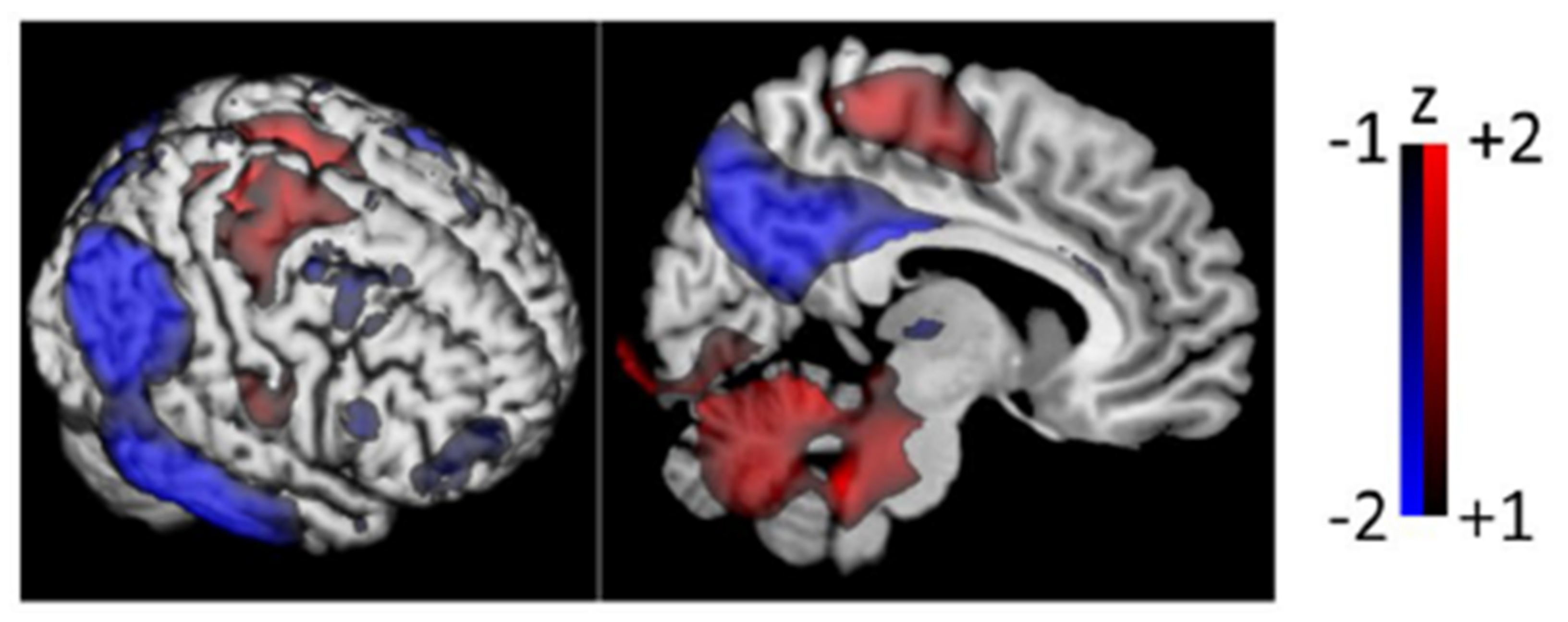
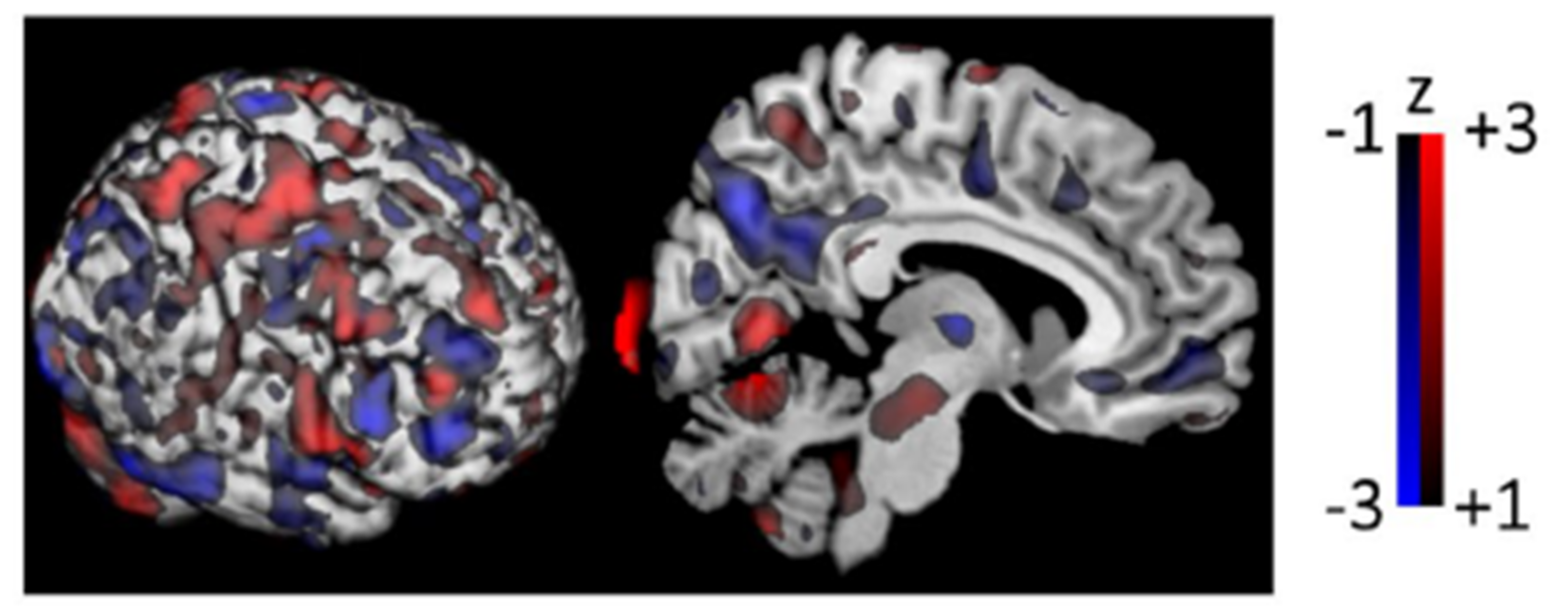
4.1. General Linear Models and Statistical Parametric Mapping

The general linear model (GLM) is a simple method for generating predictions from data. The GLM will model the response variable ( Y ) in terms of a weighted linear combination of the explanatory variables (X) and uniquely defined response parameters ( β ), plus a normally distributed error term ( ϵ ) in the form
Y M = β 1 X m 1 +     +   β X m   +     +   β L X M L + ϵ M
where there are M modeled responses and L total explanatory variables [64]. The explanatory variables may be continuous or discrete and may be any combination of features (e.g., FDG uptake in the precuneus) or covariates (e.g., age and sex). For the case of neuroimaging studies where each voxel is a feature, the number of observations is always less than the number of features/covariates, and so the GLM is an underdetermined system and cannot be explicitly solved. The model parameters are then estimated using the method of ordinary least squares,
ϵ = Y β X = Y Y ^ ,
where the hat notation refers to the estimated model values and the bold notation indicates row or column vectors of values.
Under the condition that X T X is invertible, we may uniquely solve for the least squares estimate of the parameters as
β ^ = X T X 1 X T Y .
If the parameter estimates are normally distributed, any arbitrary linear combination of these will also be normally distributed. Consider then that for some vector of weights c known as the contrast vector, a hypothesis based on Student’s t-distribution for ML degrees of freedom and using the model parameters may be written as:
T = c T β ^ c T β σ 2 ^ c T X T X 1 c ,
where σ 2 ^ is the estimated variance of the errors, defined as:
σ 2 ^ = ϵ T ϵ M L
and the null hypothesis requires that c T β = 0 . A similar expression may be obtained for generating F-statistics [64].
The extremely successful application of the GLM to the domain of neuroimaging has been enshrined in the method of statistical parametric mapping (SPM). Developed by Friston and colleagues, it is the most widely used neuroimaging analytic tool that has been used for research purposes since the 1990s [76,77]. It allows users to run voxel-wise GLM analyses and provides options for multiple comparison corrections that are tailored for neuroimaging data. The output of this mass univariate analysis is a statistical parametric map such as that seen in Figure 2—an image where voxel values are assumed to be distributed under a known probability density function (e.g., t-distribution). These maps are the primary output of SPM and are used as evidence for or against the null hypothesis at the level of the voxel [76,77]. This method of generating parametric maps has resulted in the eponymous software package known as “SPM”, of which the latest version as of publication is SPM12 (Wellcome Trust Centre for Neuroimaging, London, UK).
In SPM and many other neuroimaging analytic software programs, the images are rotated in a common direction and are spatially normalized with respect to a common stereotactic space (e.g., Montreal Neurological Institute stereotactic coordinates) to ensure spatial registration at the level of the voxel. These may also be co-registered in cases where more than one mode of neuroimaging data are available. Images are then usually smoothed with an isotropic Gaussian filter to ensure the robustness of the registration process and increase the signal-to-noise ratio of the data. Smoothing also ensures that the neighboring voxels are interdependent. Smoothing is also a necessary condition for the multiple comparison correction with Gaussian field randoms [78]. At this point, statistical inference may proceed as described above. The contrast vector may be used to generate SPMs of the hypo- or hypermetabolic regions in FDG-PET images at the level of the patient or the group. This can be used to detect AD in two primary ways. First, a visual inspection of the statistically significant regions can be performed. These statistically significant clusters may be displayed on a glass brain in the application viewer, but they may also be visualized over an anatomical template, or on subject-specific MR images. SPM will also generate tables of statistics for each significant cluster and any existing sub-clusters and allow for the modification of relevant thresholds. SPM has some notable and well-known disadvantages when compared to other methods. SPM-based analysis assumes sphericity between all possible pairs of groups under consideration. Being a mass univariate methodology, it also suffers from the multiple comparison problem, which must be adequately corrected to avoid dramatic type I errors. SPM also locates statistically significant clusters (see Equation (4)) based on a facsimile of the signal-to-noise ratio—a contrast of parameter values to their standard error—which may introduce artifactually large parameter values in regions of low noise, such as outside the brain, unless corrected with brain masking and/or intensity thresholding. SPM also assumes that the error variance-covariance is stationary under the null hypothesis. SPM and many other methodologies also require elaborate preprocessing procedures to ensure exact voxel-wise spatial correspondence between images/groups. SPM also presupposes the use of relatively arbitrary thresholds for statistical significance. Furthermore, SPM maps are best suited for subjective visual interpretation; however, masks of any statistically significant clusters may be used as a form of dimensional reduction on whole images.
It has been demonstrated that SPM-aided FDG-PET readings can improve the differentiation of AD patients from healthy controls (HC), sMCI, or pMCI patients [79,80,81,82,83,84]. SPM-aided readings may also improve the differentiation between different neurodegenerative disorders. Perani et al., found that when given SPM-generated maps, specialists performed significantly better in diagnosing dementia and were better able to differentiate between several forms of DSD, including MCI [81]. Katako et al., published a novel use of the GLM using the vector of response parameters (“beta map”) over each voxel in the image. The dot product of this with the voxel values of the proportionately scaled FDG-PET images was used to create subject-specific scores representing the similarity of the subject’s FDG-PET image to the group-derived beta map. Using this technique, they were able to reliably differentiate AD patients and HCs with sensitivity = 86.2%, specificity = 85.6%, and area-under-curve (AUC) = 0.922 [85]. Liu et al., discovered, by use of a GLM, that female subjects exhibited significantly greater accumulation of tau neurofibrillary tangles in the MCI stage compared to male subjects if they possessed the APOE-ε4 genetic mutation [86]. Ottoy et al., used a GLM to explore the effects of short-term (<1 year) conversion rates from MCI to AD states by combining FDG-PET, amyloid-PET, CSF markers, structural MRI, and neuropsychological testing information. They discovered that FDG-PET and hippocampal volume combined with neuropsychological testing best predicted short-term conversion from MCI to AD, and that neither amyloid-PET nor CSF markers were able to predict conversion [87]. Nordberg et al., performed a multi-center study of amyloid-PET imaging to investigate its value as an indicator of prodromal AD by use of a GLM using amyloid neuroimaging data and demographic and neuropsychological information [88]. The results show that MCI patients fall within a bimodal distribution of amyloid burden, as measured by [11C]PIB retention. A total of 64% of MCI patients were amyloid-positive, while the remainder were not. The data also showed that 67% of these amyloid-positive MCI patients eventually developed AD at follow-up; however, none of the amyloid-negative MCI patients were diagnosed with AD at follow-up, showing a 100% negative predictive value for amyloid-PET for AD [88]. Saint-Aubert et al., evaluated the relationship between the tau tracer [18F]THK5317, FDG uptake, and cognition using a GLM. They discovered significant negative correlations between episodic memory and overall cognition with [18F]THK5317 uptake, and that FDG uptake had a mediating effect between [18F]THK5317 uptake and overall cognition [89]. Jeon et al., used an unsupervised statistical technique known as hierarchical clustering to discover AD subtypes by integrating cortical structural MR, tau-PET, and amyloid-PET information in addition to demographic data from a population of AD patients and then comparing the results to HC patients by means of the GLM [90]. Halawa et al., discovered a significant cross-sectional correlation between functional activity questionnaires, cortical tau burden, cortical amyloid burden, and amyloid-tau interactions in MCI and AD patients through GLM modeling [91]. Ossenkoppele et al., discovered a novel spatial effect of the APOE-ε4 genetic mutation on amyloid accumulation and FDG uptake through the use of a univariate GLM. They discovered a less pronounced amyloid burden in the frontal cortices of noncarriers and a more pronounced decline in FDG uptake in the posterior portions of the brain in carriers [92]. Sörensen et al., used voxel-wise regression and determine patterns of cerebral glucose metabolism in FDG-PET images, which forecasted cognitive decline [84].

4.2. Stereotactic Surface Projection

Where SPM is a general tool for the quantitative analysis of neuroimaging studies primarily based on GLM approaches, which are agnostic to the data under investigation, three-dimensional stereotactic surface projection (3D-SSP) is a voxel-driven method that was purpose-built as a fully automated method of quantifying AD pathology from FDG-PET images [93]. Relevant to the detection and diagnosis of AD, 3D_SSP is an engineered method of extracting metabolic information from FDG-PET images that uses a priori knowledge of AD. Using data from known populations of AD and HC patients, 3D-SSP generates diagnostic indices based on Z-scores generated by voxel-wise comparisons. It has since been expanded to be applicable to DSDs in general, including mixed forms of dementia [34]; 3D-SSP is also incorporated as a primary component of the software package Neurostat® (Department of Internal Medicine, University of Michigan, Michigan, Ann Arbor, MI, USA), which is available for download online [94].
PET images will first undergo a c series of operations at the level of both the group and the subject prior to analysis. The images are rotated to ensure they are in the correct anatomical orientation and then undergo stereotactic anatomic standardization to a known template space. Regional anatomical differences are minimized by linear scaling and nonlinear warping, and the image is resampled [93]. Voxel values at predetermined locations on the outer and medial surfaces of the cerebral cortex are considered up to a depth of 6-voxels (13.5 mm) along a vector normal to the surface-most voxel. The maximal voxel value along this 6-voxel deep vector is returned as the value at the surface voxel. This set of maximum-valued voxels is then normalized to the thalamus because, it is a known region of relatively preserved metabolism in AD patients.
a c t i v i t y n o r m = a c t i v i t y m e a s u r e d / t h a l a m i c a c t i v i t y .
The mean and standard deviation of each surface voxel are then computed using a collection of FDG-PET images from HC patients. Using the same procedure, the surface voxels from the AD population are then compared to those of the HC database, and a Z-score is computed
Z A D x , y , z = H C m e a n x , y , z A D x , y , z H C s d x , y , z
on a voxel-by-voxel basis. e x , y , z are the stereotactic coordinates of a surface voxel, Z A D x , y , z is the Z-score of a surface voxel of the suspected AD patient, H C m e a n x , y , z and H C s d x , y , z are the mean and standard deviation of the surface voxel from the collection of HC controls, and A D x , y , z is the thalamic-normalized value of the surface voxel of the suspected AD patient.
An index of Z-scores is then computed for the primary cortical areas affected by AD—the frontal, parietal, and temporal cortices. The locations of these cortices are defined using predetermined stereotactic grid coordinates. Δ Z -scores are then computed by comparing Z-scores of the frontal + parietal + temporal cortices to those of the primary sensorimotor cortex,
Δ Z = Z F C / P C / T C Z S M C
such that a large difference in Z-score indicates more severe hypometabolism in the region relative to the primary sensorimotor cortex. This is performed bilaterally, where the values from each hemisphere are averaged together, and the subject may be classified as symmetric or asymmetric based on the degree of hypometabolic similarity between cortices [93].
Diagnostic indices are then determined with respect to the HC database by establishing cut-off values for metabolic abnormality based on the Δ Z -scores [93]. These may then be visualized on a subject’s MR image, an MR template, or a glass brain in a manner like SPM. After indices have been determined through the database, an individual’s neuroimaging data may be compared to that of the HC database, and a diagnostic label may be applied by a physician’s quantitatively informed impression of statistically significant differences in tracer uptake.
A distinct advantage of this method is its intrinsic motivation, based on well-known findings from FDG-PET studies on AD patients: hypometabolism in the parietotemporal cortex, bilateral symmetry of metabolic reduction, frequently reduced metabolic activity in the frontal cortex, and preservation of the primary sensorimotor cortex and thalamus [95,96,97,98]. A great advantage of this design choice is that it easily allows for the incorporation of new information on the nature or etiology of AD. Another is that the method automatically prepares and presents data-driven hypotheses in the form of a Δ Z -score in a visually interpretable manner (color-scale on a brain template), thus complementing the role of the specialist physician in the diagnosis of AD. This is, however, a potential disadvantage, as it is notably distinct from the proper diagnostic tools as the method only presents quantitative information instead of performing a classification alongside the presentation of the information. This is particularly notable when using the method for differential diagnosis of DSDs because the result remains entirely dependent on the specialist physician’s subjective impression of the spatial distribution of altered metabolism.
Most notably used as a portion of the Neurostat® (Department of Internal Medicine, University of Michigan, Michigan, Ann Arbor, MI, USA) software package, 3D-SSP has been demonstrated to increase clinician confidence and accuracy in the diagnosis of DSDs and also serve as the inspiration behind further methods of analysis on the cortical surface [99,100,101,102,103]. Most of the literature making use of 3D-SSP has been focused on the features derived from FDG-PET imaging; however, there is an increasing penetrance of amyloid and tau data into the domain of 3D-SSP. A novel use of 3D-SSP was reported by Iizuka et al., using rifampicin, a drug used to treat mycobacterium infection that has also been shown to prevent amyloid oligomerization and tau hyper-phosphorylation in mouse models [104]. Forty subjects with AD-like hypometabolism undergoing treatment for mycobacterium infection were given 12 months of treatment with 450 mg of rifampicin and showed increased or stabilized FDG uptake within the posterior cingulate cortex. Results were compared pre- and post-treatment using z-score maps derived from 3D-SSP, showing a milder decline or no further decline with follow-up FDG-PET imaging. Dual-biomarker imaging is an area of PET-based AD investigation that investigates the use of non-FDG tracers to obtain FDG-like diagnostic data. The rationale for using the first phase of the tracer update as a surrogate for FDG-PET is based on the neurovascular coupling hypothesis, which describes how glucose metabolism and oxygen demand are highly correlated in time. Daerr et al., compared the performance of FDG and the amyloid tracer florbetaben in gathering perfusion-metabolic information very early post-injection [105]. It was shown that very early florbetaben frames are very similar to data acquired in FDG-PET throughout a priori selected ROIs. Early perfusion amyloid frames (first 5 min post-injection) and FDG values were significantly corrected when normalized to the global metabolic mean in amyloid-positive (r = 0.90) and amyloid-negative (r = 0.79) patients. These data were later presented in the form of 3D-SSP z-score maps to multiple neuroradiological readers who showed high inter-reader agreement (kappa > 0.79) between AD, FTD, and HC patients. Brendel et al., published a similar report for the correspondence of FDG and the tau tracer THK5351. They discovered an extremely strong correlation between FDG and THK5351 uptake in the first minutes post-injection (dice similarity coefficient = 95%) up to 15 min post-injection (coefficient = 89%) [106]. These similarities were visually confirmed by a neuroradiological reader presented with z-score SSP maps generated from FDG and THK5351 data. Brendel et al.’s study was performed on a single patient as a pilot project. Beyer et al., performed a larger experiment with 26 subjects across a variety of DSDs on the second-generation tau tracer PI-2620 [107]. As in Daerr et al., Brendel’s study used multiple readers of different levels of experience to evaluate the subjective similarities of FDG-PET and early perfusion PI-2620 using Neurostat® (Department of Internal Medicine, University of Michigan, Ann Arbor, MI, USA). The greatest single frame correlation (r = 0.744) occurs between the tracers occurred in the 30 s following the first minute post-injection, and they report that combining frames reveals an optimal timing window from 0.5–2.5 min post-injection (r = 0.728) [107]. Thientunyakit et al., were the first, to the author’s knowledge, to apply 3D-SSP on florbetapir amyloid-PET images with a population of 31 AD, 27 MCI, and 20 HC patients [108].

4.3. Principal Component Analysis & Scaled Subprofile Modeling

GLMs are a data-agnostic tool, and 3D-SSP is a highly engineered method for AD detection and diagnosis, but they may both have difficulties when working with very intercorrelated and/or high-dimensional data sets. Principal component analysis (PCA) is a widely known technique of multivariate analysis and is commonly used as a means of dimensionality reduction [109]. PCA is used to reduce a large dataset to a small number of orthogonal variables that carry a majority of the variance within the data. This is accomplished by finding a new linear vector basis on which to re-express the data such that the data are decorrelated, the variance is maximized, and the reconstruction error is minimized. This is easily expressed in matrix notation as:
Y = P X
where Y is the decorrelated matrix, P is a transformation matrix, and X is the original dataset.
Consider a dataset in the form of a matrix X with I rows and J columns corresponding to the number of observations and the number of variables describing those observations, respectively. Let us now define the covariance as the degree of linear relationship between two variables (the columns of X ), written as:
C X = X X T
where we assume the dataset is standardized to the number of observations, zero-centered, and with unit variance. The covariance of the decorrelated matrix should have two relevant properties: (1) all off-diagonal terms should be zero, and (2) each diagonal term should be ranked in order of decreasing variance. Thus, the goal of PCA is to find an orthonormal matrix P , such that C Y is a diagonal matrix. The rows of P will then be the principal components (PCs) of X . See Figure 3 for a visualization of these principal components.
Consider the form of the covariance matrix C Y is written:
C Y = Y Y T = P X P X T = P X X T P T = P C X P T .
This symmetric matrix may be diagonalized by multiplication with an orthogonal matrix of its eigenvectors,
C X = E D E T
where D is a diagonal matrix and E is the matrix of eigenvectors. Thus, if we choose our transformation matrix P to have rows composed of the eigenvectors of C X we may write
C Y = P C X P T = P E T D E P T = P P T D P P T = P P 1 D P P 1 = D .
The construction of eigenbrains (aka eigenimages) have demonstrated their utility as a tool for reducing the dimensionality of the feature space to a simpler set of projection coefficients [110].
A further extension of PCA is scaled subprofile modeling (SSM). SSM generates a group-level score that represents disease-specific patterns. SSM has as an underlying assumption that neuroimaging data represent the brain as a set of spatially distributed but interconnected regions. This leads to the assumption that metabolic processes give rise to specific patterns of metabolic covariation across these regions that are characteristic of a group-level pattern in regional cerebral metabolic rates of glucose consumption [111].
We now assume that the data are organized in a dataset matrix P such that every row corresponds to a subject and every column refers to a unique voxel of that subject’s neuroimaging data, forming a matrix of dimension S × V . We also assume that the data have been spatially normalized to a common template place, smoothed, and that an intracranial mask has been applied. The subscripts s and v denote subject- and voxel-wise measurements.
The data are first log-transformed and then centered with respect to the log-mean value of glucose metabolic rate,
Q s v = log P s v L G M R s L G M R s = m e a n v log P s
resulting in “row-centered” (subject-wise) data. These data are then “column-centered” (voxel-wise) by subtracting the mean value of a voxel over the entire subject group,
S R P s v = Q s v G M P v
where G M P (group mean profile) and SRP (subject residual profile) are defined:
S R P s v = Q s v G M P v G M P v = m e a n s Q s v .
A subject centering scalar is defined as the difference between the subject-wise mean of the logarithmic group metabolic rate (LGMR) and the group-wise mean of LGMR,
c C s = L G M R s m e a n s L G M R s ,
where c C s is defined as the subject centering constant. (17) may now be explicitly rewritten,
S R P s v = log P s v m e a n s log P s v m e a n v ( log P s ) m e a n s ( log P s ) .
In this form, we note that the SRP at the level of the voxel is representation of the difference between the log values of the subject and the appropriate group mean.
At this point, a singular value decomposition (SVD) is performed on the voxel- and subject-wise covariations of the SRP. An SVD is a generalization of the diagonalization of a matrix by its eigenvectors. We first define the subject-wise covariance matrix,
S s = S R P S R P T ,
and then by multiplying the eigenvalue relation S s e k = λ k e k by S R P T from the left we may write:
S R P T S R P S R P T e k = λ k S R P T e k
where the subscript k refers to the size of the set of eigenvalues.
Note well here that the product of the matrix multiplication S R P T S R P is the voxel-wise covariance matrix S v . We note that in (20), this matrix has eigenvectors S R P T e k , which carries a special significance in SSM methodology and is known as the group invariant subprofile (GIS) vectors. As such, we may rewrite (20) as:
S v G I S k = λ k G I S k ,
where S v = S R P T S R P and G I S k = S R P T e k . From here we define and compute a subject score by multiplying each of the normalized eigenvalues by their associated and normalized eigenvector,
s c o r e k = λ k e k .
The SRP is then easily expressible as a linear combination of orthogonal GIS vectors weighted by their associated subject score,
S R P s = k s c o r e k s G I S k .
The metabolic profile at the level of a subject is therefore expressed in terms of group-level parameters.
The major strengths of both PCA and SSM are their abilities to expressly quantify the relative importance of each dimension of the decorrelated data with measures of their variance. It also provides a means for describing a complex and highly intercorrelated dataset with a much smaller number of decorrelated variables and is thus an important method of dimensionality reduction. The computation of the PCs is also quite straightforward since nearly all high-level programming languages have built-in functionality for computing eigenvectors of matrices or performing SVD [109]. SSM is notable for its use of log-transformation and double centering, which allow the method to explicitly separate subject-dependent and regional scaling effects. GIS patterns are thought to express “small signals” processes, and thus true descriptions of disease-specific abnormalities. GIS patterns are also constant throughout disease progression, whereas regional metabolic patterns (such as those revealed by mass univariate methods) change with disease progression. This shows that there exists a distinction to be made between SSM and regional metabolic pattern; however, it has been recently shown that SPM and SSM/PCA are, in fact, not independent of one another and have a well-defined analytical relationship when performed on FDG-PET of AD patients [111,112,113]. In either PCA or SSM, analysis at the level of the single subject is straightforward and involves taking the dot product of each FDG-PET image with the PCs, or else taking the dot product of the scaled subprofile of a patient’s FDG-PET image with the PCs—both of which will generate a quantitatively meaningful subject-specific score that may be used to differentiate patient groups. Furthermore, GIS vectors are determined to represent true disease-specific metabolic patterns, which may be visualized in the form of Z-scores, such as in 3D-SSP, and used to model group-specific abnormalities in brain glucose metabolism. This is especially useful because these are invariant group characteristics, whereas the subject score is indicative of disease expression [112]. PCA is also very amenable to unsupervised machine learning in cases where differences in class label are not considered; however, PCA is often ill-suited for non-linear data. The stepwise linear regression is also useful in contexts where single PCs are insufficient [85,114]. PCA is also a well-established means of reducing feature complexity during data preprocessing operations and can be used to eliminate unnecessary or redundant information.
By using two different SSM-based classifiers (first PC vs. multiple PCs), Katako et al., were able to differentiate AD and HC patients with sensitivities and specificities of 78.7%/81.9% and 80.2%/86.5%, respectively, and AUCs of 0.852 and 0.911 [85]. Teune et al., have also discovered distinct Alzheimer-related glucose metabolic patterns that had 93% sensitivity and 94% specificity for correctly classifying AD between probable AD patients and those with MCI [115]. Iizuka & Kameyama were able to use SSM-PCA to dis metabolic profiles, which differentiated dementia with Lewy bodies (DLB) and AD with AUC = 0.937 [116]. Meles et al., also used SSM to develop a discriminator for pMCI and HC groups with sensitivity = 82.4% and specificity = 85.7% [117]. Substantial work has been done in applying PCA/SSM models to amyloid- and tau-PET data. Blazhenets et al., reported a study on 319 MCI subjects that explored the use of imaging and non-imaging data to predict MCI to AD conversion [118]. By applying SSM-PCA to amyloid images of sMCI and pMCI subjects from the Alzheimer’s Disease Neuroimaging Initiative (ADNI), they used logistic regression to select PCs with the greatest explanatory power at follow-up. Results reported from an independent test set using combined FDG, amyloid, and non-imaging variables showed significant group separation between converters and non-converters using the PCs obtained through SSM-PCA and Cox voxel-wise regression. A further follow-up study in 2021 from the same group reports that their model has strong predictive power in estimating the risk time to conversion from MCI within the AT(N) framework [119]. Yokoi et al., used SSM-PCA on combined fMRI and tau-PET data on amyloid-positive patients and discovered a spatially dependent pattern of tau retention within patient group precunei, posterior cingulate cortices, and dorsolateral prefrontal cortices [120]. This pattern had 82.6% specificity and 79.1% sensitivity in differentiating AD HC patient groups. A positive correlation between tau retention and canonical resting-state functional networks was also discovered, but a negative correlation was reported between tau retention and seed-based analysis originating in both the precuneus/PCC and left dorsolateral prefrontal cortex. Perovnik et al., used SSM-PCA to identify an Alzheimer’s-related pattern from a combination of FDG-PET images, CSF protein markers, and neuropsychological information in a group of 20 AD and 20 HC subjects. The pattern was then validated on a group of 261 patients with AD, a behavioral variant of frontotemporal dementia (bvFTD), MCI, and HC subjects. They report differentiating AD HC groups with AUC = 0.95 and MCI vs. bvFTD from AD with AUC = 0.76 to 0.85 between internally and externally validated sample groups [120]. Perovnik et al., also used SSM-PCA to develop a disease-specific pattern to differentiate DLB from AD patients with an AUC = 0.87. This result is notable due to the significant clinical comorbidity of DLB and AD symptoms [121]. Peretti et al., used SSM-PCA to generate disease-specific patterns for AD from amyloid-PET images [122]. They reported that amyloid-PET images were sufficient to differentiate between healthy controls and AD patients, but that FDG-PET or regional cerebral perfusion-weighted images were necessary to distinguish between AD, pMCI, and sMCI groups with statistically significant accuracy, leading them to suggest that perfusion-weighted images can be used as a surrogate for FDG-PET when performing SSM-PCA analysis.

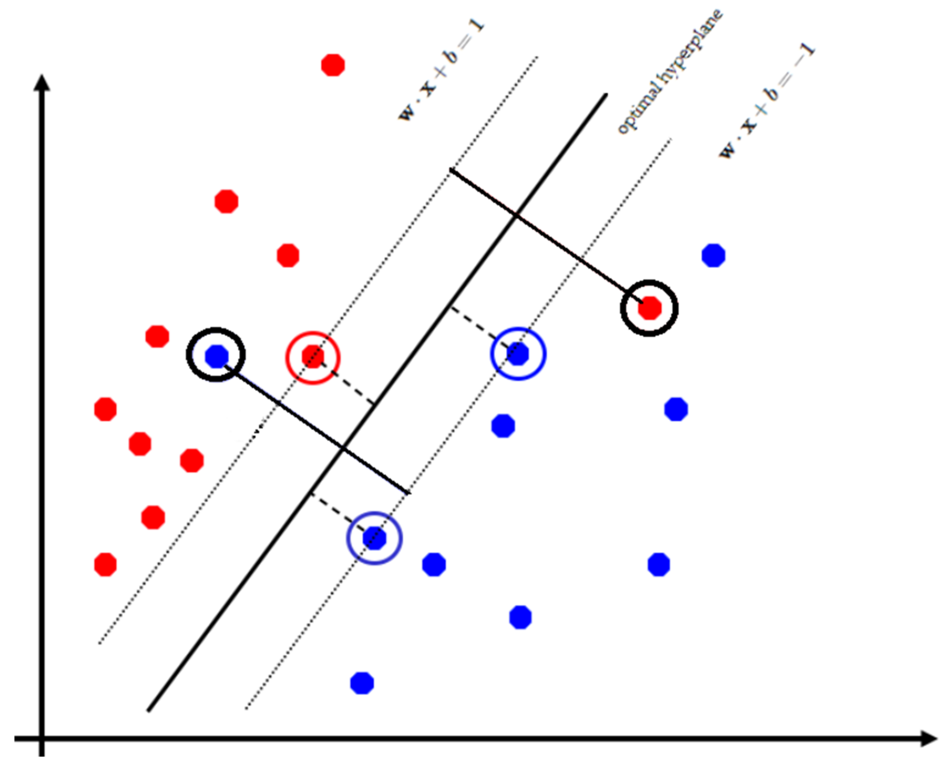
4.4. Support Vector Machines

We will now introduce the support vector machine (SVM). SVMs are exceptionally common in the neuroimaging literature. They differ significantly from GLMs or PCA/SSM in that no threshold score is used to determine group designation, but rather the sign of the score is used in determining the group label.
The theoretical foundation of the SVM can be simply explained by the statement “a 2D space is clearly separable by a 1D line”. This is also intuitively true for the separation of a 3D space by a 2D plane. This property holds for spaces of arbitrary dimension: a hyperspace of N-dimensions is separable by a linear hyperplane of N-1 dimensions [123].
Consider some arbitrary dataset,
x 1 , y 1 , x 2 , y 2 , , x n , y n
where x i is a p-dimensional feature-vector and y i is a binary label classifying the vector. An SVM will separate these feature vectors according to their class by attempting to find the geometric margin (a hyperplane) that maximizes the minimum distance between classes.
The optimal hyperplane is defined as the set of points that satisfy:
H = x | w T b + b = 0
where w is a vector normal to the hyperplane and b is a bias. All vectors having a magnitude H 1 or H 1 belong to the positive and negative classes, respectively, but those with the special property H = 1 are designated support vectors. The support vectors determine the placement of the hyperplane, and the SVM optimization algorithm will attempt to construct the hyperplane using the support vectors that are as far away from one another as possible, as seen in Figure 4 and visualized in Figure 5. This is a minimization problem that has the form:
min w ,   b   w T w   s . t .     i   y i w T x + b 1 .
Note that when support vectors are of unit length, the width of any hyperplane is determined by 2 w , therefore minimizing the magnitude of w maximizes the separation between classes.
Most data are not linearly separable or are sufficiently low in dimensionality that there is no optimal boundary that separates all vectors. For these cases, we may introduce a “soft-margin” optimization by allowing a slack variable ( ζ ) and a regularization constant (C) in (28), such that:
min w ,   b   w T w + C i = 1 n ζ i       s . t .     i   y i w T x + b 1 ζ i     s . t .     ζ i 0 .
In this form, the classifier will allow feature vectors to exist on the “wrong” side of the hyperplane without affecting the shape of the boundary. Larger values of C penalize the optimization and often make for a highly non-linear classification boundary, whereas smaller values of C allow for a simpler boundary less prone to overfitting the data.
Note that in (26), the optimization considers the inner product of the vector orthogonal to the hyperplane. Any other mathematical function expressible as an inner product may be chosen in its place; thus, another solution to the problem of the non-linear boundary is to artificially increase the dimensionality of the data by appropriate choice of kernel function. This is known as the “kernel trick”. The radial basis function (RBF)
R B F x , x = exp x x 2 2 σ 2 ,
is a very common choice for this purpose since it may express data over a continuous range and therefore as infinite effective dimensionality [123]. Choice of kernel for exploiting the “kernel trick” is sensitive to the nature of the data and results can vary.
SVMs are quite amenable to incorporating regularization methods into the optimization process. They may also undergo k-fold cross-validation. Both regularization and cross-validation can help prevent overfitting [85]. SVMs may, however, be easily confounded by overlapping or noisy datasets and may underperform when the number of features is larger than the number of training samples. Noisy datasets may, however, be more accurately differentiated through one-class SVMs. SVM hyperplanes may also be difficult to interpret since they may be very high-dimensional. SVMs also do not output any probabilistic information related to the classification label because they are intrinsically binary classifiers. Classification tasks with more than two labels necessitate training multiple binary classifiers for each pair of cases. SVMs are highly effective in high-dimensional spaces and perform optimally on linearly separable data. The optimization algorithms are also quite mature and highly efficient in their use of computational resources [124].
After determining the optimal hyperplane separating each group, an FDG-PET image may be vectorized (AKA flattened) and fed into an SVM for classification. This remains a very common way of using SVMs on image-based data because this method is extremely amenable to feature selection/engineering practices and to the concatenation of additional features along this voxel-vector (data fusion). Using two different forms of SVM-based classifiers (the iterative single-data algorithm and sequential minimal optimization), Katako et al., were able to test two forms of SVM for classifying different patient groups. In classifying AD vs. HC, they achieved the best performance with the iterative single-data algorithm SVM (AUC = 0.945, sensitivity = 0.840, specificity = 0.955), whereas for classifying sMCI vs. pMCI, they reported a combined performance (sensitivity × specificity) of 0.590 on a privately curated dataset [85]. Illan et al., were able to classify AD vs. HC patients using a SVM classifier and PCA-based data preprocessing that performed with sensitivity = 88.64%, sensitivity = 87.70%, and accuracy = 88.24% [125]. Ramirez et al., were able to achieve 90.38% accuracy on the same task using raw image data (voxels as features) [126]. Garali et al., were able to introduce a feature selection algorithm that used 21 regions from FDG-PET images to achieve 95.07% accuracy on AD vs. HC classification using SVM [127]. Hammes et al., developed an SVM-based classifier that used 18F-flortaucipir tau-PET data and SSM-PCA [128]. They showed that their classifier and tracer were able to differentiate between amyloid-positive and amyloid-negative, typical and atypical AD patients, and FTD. Their classifier was also able to predict amyloid positivity with an AUC = 0.952 [128]. Damasceno et al., used the colocalization of amyloid and tau burden in a cohort of amyloid-positive patients for an SVM classifier. They constructed a feature vector containing a mean standardized uptake ratio (SUVR: ratio of observed tracer uptake to that of a standardized reference region), cortical thickness from MR, and the product of amyloid and tau burden for each ROI. It was determined that this combination of features outperformed each individual feature set and was able to differentiate between patients with MCI, AD, and non-AD dementias (progressive cortical atrophy and lopogenic variant primary progression aphasia) with an AUC approaching 0.9 [129]. Syaifullah et al., published research on an SVM-based classifier that used amyloid PET and structural MR data to predict conversion from MCI to AD with 87.2% accuracy, 81.7% sensitivity, 90.1% specificity, and an AUC = 0.94 [130]. Ding et al., were able to use amyloid PET data in combination with CSF protein markers, neuropsychological scores, and an SVM classifier to achieve AD vs. HC classification with AUC = 0.93 and sMCI vs. pMCI with AUC = 0.83 [131]. Varatharajah et al., investigated a series of quantitative methods for predicting conversion from MCI to AD from FDG-PET, CSF amyloid and tau markers, structural MRI, mini-mental state examination (MMSE) scores, a measure of cognitive resilience, genetic data, and demographic data. It was determined that linear kernel SVM outperformed multi-kernel learning SVM and GLM with elastic regularization in this task with sensitivity = 0.93, specificity = 0.77, accuracy = 0.81, and AUC = 0.93 [132]. Zhao et al., used longitudinal FDG-PET images to predict MCI to AD conversion and achieved an accuracy of 89.9% with an AUC of 0.892 [133]. Their work made use of a novel brain atlas (Brainnetome Atlas), a novel normalization procedure, and an engineered distance metric for their network [134,135]. Furthermore, their work is unique for making use of ADNI subjects with four separate FDG-PET studies.

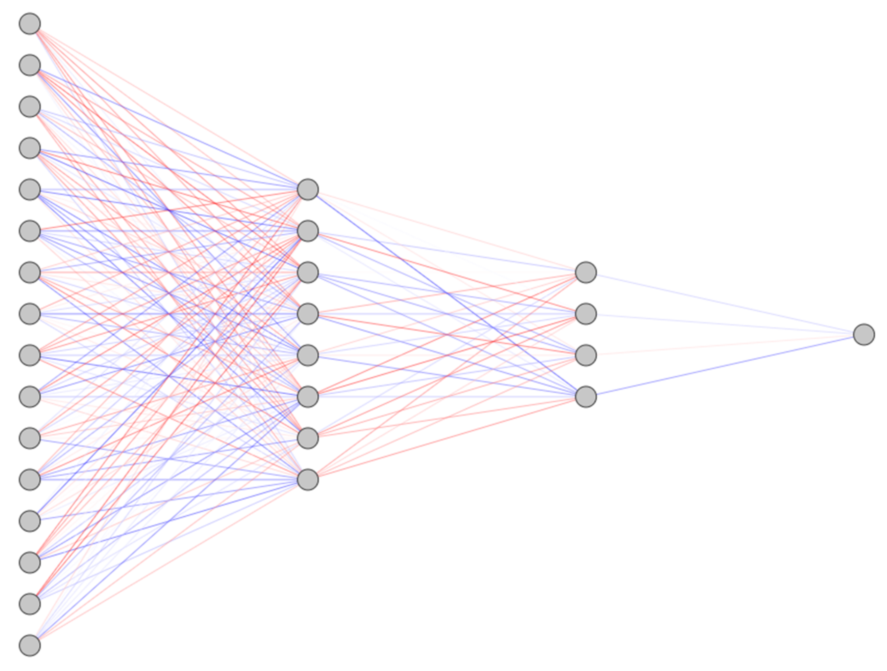
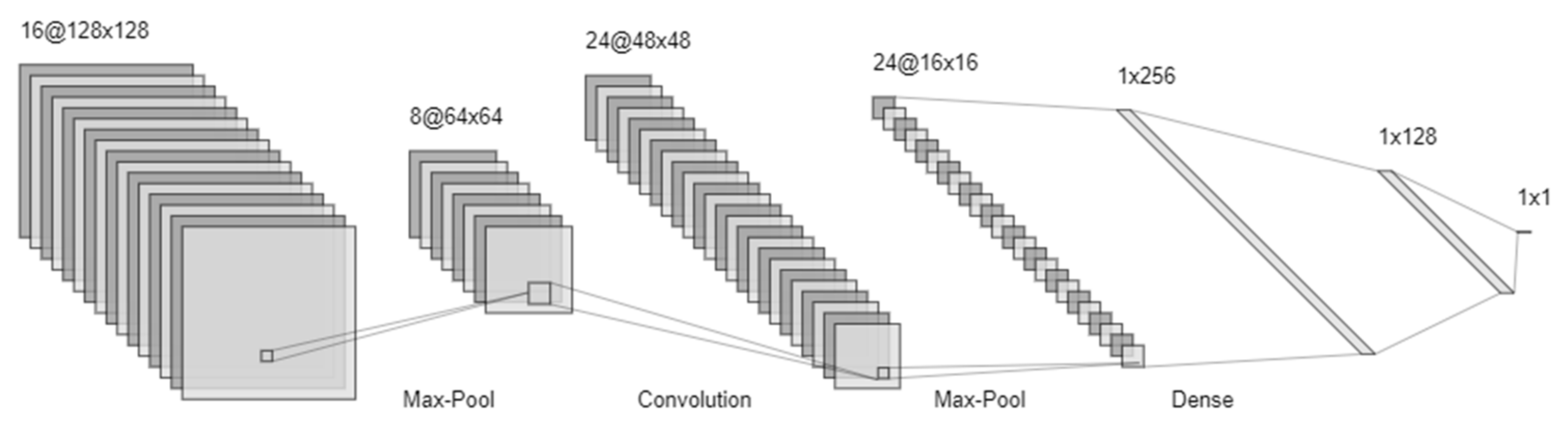
4.5. Neural Networks

SVMs are highly valued tools for data classification; however, they are impaired by difficulty in finding the optimal hyperplane when the number of observations is small compared to the number of features or when the data are highly non-linear. Neural networks (NNs) are the result of attempts to recreate the information processing structures found in real brains. Much like how brains may be naively viewed as combinations of neurons and axons, a NN is therefore easily conceptualized as a combination of nodes and connections that are organized into layers. These layers are broadly classified into input, hidden, and output layers. The input layer is where data may enter the network. The hidden layers form the bulk of the architecture and perform mathematical transformations on the input data as it passes through the network. The output layer is necessarily the final layer of the network and will output a label in the case of classification networks or a number in the case of regression networks [136,137]. NNs are very well-suited to modeling non-linear data, unlike the methods previously discussed.
Nodes are the sites of mathematical transformations in the network. At a node, we consider the values input from the previous layer, the weight of the connection along which this value has traveled, and the bias value for the layer (see Figure 6 for a visualization of a common NN architecture). Consider that the summation at some hidden layer in a NN may be written as:
a = ρ w T x + b
where a is the vector of activations (output values of the layer), w is the vector of connection weights, b is the scalar bias of the layer, x is the input data, and ρ denotes some non-linear function. The most common non-linearity (AKA activation function) is the rectified linear unit (ReLU); however, both the sigmoid and hyperbolic tangent functions are still widely in use [138]. At the time of feeding the final activation values forward into the output layer, the values will be passed through an output function. The softmax function,
σ z = exp z i a exp z a ,
is a common choice and generalizes both the binary and multi-class tasks. The softmax function also has a very evident probabilistic interpretation. Other functions are also widely used, such as the mean squared error or the Manhattan metric.
A convolutional neural network (CNN) is an extension of the fully connected network explained above that uses convolution operations throughout its hidden layers to transform image-based data [136,137].
A convolutional layer is an ensemble of filters that act upon the image and are defined by several quantities such as kernel size (AKA receptive field) and stride (number of voxels skipped between each convolution). The output of a convolutional layer is a series of feature maps, one for each of the filters used at the convolutional layer. Dimensional reduction of the data being passed through the network is often performed with pooling operations, such as average and maximum pooling, which may also be used to reduce the size of the image matrix between layers [136]. CNNs also use non-linearities between layers to model non-linear relations within the data. CNNs may also contain one or more fully connected layers that are usually found at the end of the network architecture. The input to these layers is the flattened feature maps computed from the final convolutional/pooling layer. A loss function is used in conjunction with these final layers to compute any errors that exist between the network’s prediction and the ground-truth label (in the case of supervised learning) [136]. These errors are interpretable as losses that are to be minimized in the network’s training (learning) phase. The softmax function is, again, a very popular choice of loss function. Figure 7 gives a representation of a simple CNN architecture containing convolutional, pooling, and fully connected layers.
In contrast to a network’s hyperparameters, which are set by the user, the learnable parameters are those that are modified in response to the error computed at the loss layer, often as the difference between the network prediction and a known label. The loss is minimized by use of gradient descent [136,137,139].
CNNs are, however, not the only type of deep neural network, but rather the most well-known, especially in the neuroimaging research community. The recurrent neural network (RNN) model inputs vary over time or even space and are rapidly becoming more common in neuroimaging literature [140]. Generative adversarial networks (GANs) are a type of generative model that learns the distribution of training images and has been utilized for PET-based AD image classification [141]. The common theme in GANs and RNNs is using convolutional operations upon an input image and backpropagation by gradient descent to learn filter weights, reduce the dimensionality of an image, often with the point of producing a classification label [139,140].
CNNs have been widely applied for the detection and diagnosis of AD from neuroimaging studies. Liu et al., used an ensemble of RNNs to classify AD vs. HC subjects with 91.2% accuracy, 91.4% sensitivity, 91% specificity, and AUC = 0.953 using FDG-PET images. The same were also able to differentiate MCI from HC patients with an accuracy of 78.9%, a sensitivity of 78.1%, a specificity of 80%, and an AUC of 0.839 [142]. Ruwanpathirana et al., compared the performance of voxel-wise linear regression (GLM) and a CNN in modeling spatial dependencies between tau-PET and amyloid burden throughout the brain. They discovered that the CNN outperformed the GLM in predicting amyloid centiloid values and found previously unknown associations between tau topography and overall amyloid burden [143]. Ding et al., created a network based on the Inception v3 architecture, which differentiated between AD, MCI, and non-AD/non-MCI FDG-PET images with AUCs of 0.92, 0.63, and 0.73, respectively [144]. Most importantly, this network significantly outperformed radiology readers in identifying AD and MCI subjects from FDG-PET images. Guo et al., were able to develop a graph convolutional network that differentiated between AD and HC subjects with 93% accuracy and between AD, MCI, and HC groups with 77% accuracy [145]. Choi and Jin reported 96% in AD vs. HC classification and 84.2% in differentiating pMCI vs. sMCI by using vanilla 3D CNN architecture [146]. Yee et al., used a residual neural network on FDG-PET data to differentiate between AD and HC with an accuracy of 93.5% and an AUC of 0.976. They were also able to differentiate between pMCI vs. sMCI patients with 74.7% accuracy and AUC = 0.811 [147]. Pan et al., developed a multi-scale pyramidal network that prognosticated cognitive decline (MCI to AD) with 83.05% accuracy [148]. Etminani et al., developed a 3D CNN that differentiated DLB, AD, and MCI groups with AUC = 0.962, 0.964, and 0.714, respectively [149]. Hojjjati et al., constructed an artificial NN from FDG-PET and MRI features to model neuropsychological test scores for the HC, sMCI, pMCI, and AD groups. They were able to show significant differences between test scores dependent on group label and discovered that average FDG-PET values per ROI outperformed AV-45 in classification accuracy when combined with resting-state functional magnetic resonance imaging (rs-fMRI) [150]. Choi et al., were able to predict MCI to AD conversion with an AUC of 0.89 by using a deep convolutional network combining both amyloid-PET (tracer AV-45) and FDG-PET imaging data [151]. The outputs of their network were also significantly correlated with longitudinal changes in clinical dementia rating at 1 and 3 years, functional activity questionnaires, and MMSE scores. Ryoo et al., used a network based on the conditional variational autoencoder architecture and discovered four distinct subtypes of AD from FDG-PET, amyloid PET, tau PET, CSF protein biomarkers, clinical, demographic, and genetic information [151]. They also discovered differences in disease progression, clinical outcome, and demographic associations specific to each subtype. The most notable being that each subtype had a statistically significant difference in their rate of conversion from MCI to AD. Jo et al., developed a 3D CNN trained on tau PET images to distinguish between the AD HC group with sensitivity = 95.4%, specificity = 96.9%, and accuracy = 96.2%, and also between the MCI and HC groups with sensitivity = 48.6%, specificity = 82.4%, and accuracy = 64.2% [152]. They used layer-wise relevance propagation (LRP) to generate “heat maps” of the diagnostically relevant features that drive network classification [153]. These LRP maps were reported to be similar to the group-based differences shown with conventional SPM analysis. Lu et al., used dual-task learning to increase the ability of their multi-scale deep learning network to predict conversion from MCI to AD [154]. Their model performed sMCI vs. pMCI classification with an accuracy of 82.51% from FDG-PET images. Shen et al., used an unsupervised network to pretrain their NN architecture as a feature extractor and then fed the resulting feature vector into an SVM for classification in a hybrid CNN-SVM architecture [155]. Using a radial-basis function kernel in the final classifier, they achieved an accuracy of 86.6% in predicting conversion from MCI to AD.

5. Discussion

We have discussed the biological spectrum of AD pathogenesis under the ATN model and surveyed the brain structures affected by AD. We have also reviewed PET tracers sensitive to AD-specific proteinopathies (amyloid and tau proteins) and neuronal injury (FDG), considered the basic principles of tracer design, and provided references to the literature on next-generation PET tracer design. We have also presented a comprehensive examination of the most common and important data-driven methods for detecting AD neuropathology from PET imaging data and a broad survey of the uses for these methods in allied research investigating AD with neuroimaging data. A summary of the applications of these to AD identification and prognostication studies has been compiled in Table 1, where all studies reporting sensitivity, specificity, accuracy, AUC, or some combination thereof, are considered.
NNs have been criticized for their lack of transparency [156]. This is a legitimate concern considering that the result of a NN forward run is the accumulation of very elaborate mathematical transformations from the beginning to the end of a network that are neither readily interpretable by the user nor explained by the network. To this end, many visualization methods have been developed to aid in interpreting NN outputs, such as layer-wise relevance propagation or class activation mapping [153,157]. Another valid criticism of NN is their extremely data-hungry nature. These networks require enough representative examples to learn the underlying structure of the task for which it is being trained. Such data may be extremely difficult to acquire or very rare, or simply too costly to acquire. Even when sufficient data is available, the architecture under consideration may require very large computing times and computing power in order to train. Training a large-scale neural network requires several days or even weeks of training time on multiple GPUs in parallel; however, many small-scale networks can be trained in a matter of hours with appropriate hardware (e.g., a consumer-grade GPU). Transfer learning is a popular solution to this issue and applies a pre-trained network to a new training sample as a fine-tuning operation (e.g., a network trained to differentiate between cats and dogs will likely have image recognition capabilities that could be used to say distinguish between ships and trucks) [158,159,160,161]. The variety of available network architectures is a great strength of the NN as a quantitative tool. The most important classes of architecture include fully connected multilayer perceptrons, deep convolutional networks with many convolution filters, recurrent networks that examine patterns in data over space or time, long short-term memory networks that take advantage of “training example experience”, autoencoders that can reconstruct data to an accuracy that varies based on the quality of their training data, and adversarial networks that attempt to fool one another in discriminating between real and synthetic data [135,136,138,139,140,162,163,164,165]. Like other forms of machine learning, deep learning methods such as NN are also prone to the problem of overfitting; however, many strategies exist to counteract this, such as batch normalization, regularization, dropout, drop-connect, and early stopping methods [166,167,168]. Perhaps the most significant advantage of NN as a method is the lack of feature engineering. Whereas traditional machine learning methods were forced to handcraft features for consideration by a computationally intelligent algorithm (e.g., SVM), an NN with sufficient capacity is capable of extracting features without any special consideration and even of performing complicated tasks such as image segmentation or preprocessing operations [169,170,171,172,173,174,175]. NNs may also serve as feature extractors, with the output being fed into another classifier like an SVM [155].
One caveat is the lack of neural network studies that validate themselves against multiple forms of neurodegenerative dementia disorders, which are now commonly performed in models based on PCA or SSM methods [116,121,122]. This is important considering post-mortem studies which show AD diagnosis to be quite nonspecific and increase the cost of care [2,3,4,176]. Another is the demographic homogeneity of the subject population of the routinely used ADNI dataset [177]. This is being addressed through the increasing availability of online neuroimaging datasets, such as the creation of the Japanese Alzheimer’s Disease Neuroimaging Initiative (JADNI) and the Worldwide Alzheimer’s Disease Neuroimaging Initiative (WADNI), and several European neuroimaging initiatives [178,179,180,181]. A further issue with current research is the lack of explicitly stated collaboration between scientific/engineering and clinical faculty, possibly owing to difficulties of data sharing and privacy, and the lack of integration engineering and computer science specialists within clinical departments.

6. Conclusions

Neural networks continue to earn their place as the most sophisticated and accurate quantitative tool for the data-driven detection of AD neuropathology. Most interestingly, they function very well in conjunction with other classifiers and are readily amenable to single-session, longitudinal, and multimodal information. Next-generation PET tracers with increased specificity for amyloid or tau and their associated isoforms should also contribute significantly to research in this field. The present trend in the field of AD detection using neuroimaging appears to be the increasing use of neural networks, alone or in combination with other classifiers, and the fusion of multiple modalities of diagnostic data for classification, which include functional neuroimaging, structural neuroimaging, demographic data, clinical data, and even genetic data. Longitudinal data appears to be the most effective for predicting the progression of dementia due to AD in MCI patients, and single-session datasets appear sufficient for differentiating AD patients from healthy controls or even MCI patients.

Author Contributions

Conceptualization, J.P. and J.H.K.; methodology, J.P.; investigation, J.P.; resources, J.P.; data curation, J.P. and J.H.K.; writing—original draft preparation, J.P.; writing—review and editing, J.P. and J.H.K.; visualization, J.P.; supervision, J.H.K.; funding acquisition, J.P. and J.H.K. All authors have read and agreed to the published version of the manuscript.

Funding

This research was funded by Natural Sciences and Engineering Research Council of Canada (RGPIN-2016-05964), the University of Manitoba Research Program (#55127), University of Manitoba Tri-Agency Bridge Funding (#57289), the Alzheimer Society of Manitoba, the McCrorie-West Family Fellowship (#44172), and the Baxter Foundation.

Institutional Review Board Statement

Ethics approval for this study was granted by the Human Research Ethics Board at the University of Manitoba.

Informed Consent Statement

Not Applicable.

Data Availability Statement

Not Applicable.

Conflicts of Interest

The authors declare no conflict of interest.

References

  1. Arvanitakis, Z.; Shah, R.C.; Bennett, D.A. Diagnosis and management of dementia. JAMA 2019, 322, 1589–1599. [Google Scholar] [CrossRef] [PubMed]
  2. Beach, T.G.; Monsell, S.E.; Phillips, L.E.; Kukull, W. Accuracy of the clinical diagnosis of Alzheimer disease at National Institute on Aging Alzheimer Disease Centers, 2005–2010. J. Neuropathol. Exp. Neurol. 2012, 71, 266–273. [Google Scholar] [CrossRef] [PubMed] [Green Version]
  3. Brunnström, H.; Englund, E. Clinicopathological concordance in dementia diagnostics. Am. J. Geriatr. Psychiatry 2009, 17, 664–670. [Google Scholar] [CrossRef] [PubMed]
  4. Scheltens, P.; Rockwood, K. How golden is the gold standard of neuropathology in dementia. Alzheimer’s Dement. 2011, 7, 486–489. [Google Scholar] [CrossRef] [PubMed]
  5. Ward, A.; Tardiff, S.; Dye, C.; Arrighi, H.M. Rate of conversion from prodromal Alzheimer’s disease to Alzheimer’s dementia: A systematic review of the literature. Dement. Geriatr. Cogn. Disord. Extra 2013, 3, 320–332. [Google Scholar] [CrossRef] [PubMed]
  6. Petersen, R.C. Mild cognitive impairment. CONTINUUM Lifelong Learn. Neurol. 2016, 22, 404. [Google Scholar] [CrossRef] [Green Version]
  7. Sperling, R.A.; Aisen, P.S.; Beckett, L.A.; Bennett, D.A.; Craft, S.; Fagan, A.M.; Itwatsubo, T.; Jack, C.R.; Kaye, J.; Montine, T.J.; et al. Toward defining the preclinical stages of Alzheimer’s disease: Recommendations from the National Institute on Aging-Alzheimer’s Association workgroups on diagnostic guidelines for Alzheimer’s disease. Alzheimer’s Dement. 2011, 7, 280–292. [Google Scholar] [CrossRef] [Green Version]
  8. Eschweiler, G.W.; Leyhe, T.; Klöppel, S.; Hüll, M. New developments in the diagnosis of dementia. Dtsch. Ärzteblatt Int. 2010, 107, 677. [Google Scholar] [CrossRef]
  9. Van Maurik, I.S.; Zwan, M.D.; Tijms, B.M.; Bouwman, F.H.; Teunissen, C.E.; Scheltens, P.; Wattjes, M.P.; Barkhof, F.; Berkhof, J.; van der Flier, W.M. Alzheimer’s Disease Neuroimaging Initiative. Interpreting biomarker results in individual patients with mild cognitive impairment in the Alzheimer’s biomarkers in daily practice (ABIDE) project. JAMA Neurol. 2017, 74, 1481–1491. [Google Scholar] [CrossRef]
  10. De Wilde, A.; Maurik, I.S.; Kunneman, M.; Bouwman, F.; Zwan, M.; Willemse, E.A.; Biessels, G.J.; Minkman, M.; Pel, R.; Schoonenboom, N.S.; et al. Alzheimer’s biomarkers in daily practice (ABIDE) project: Rationale and design. Alzheimer’s Dementia Diagn. Assess. Dis. Monit. 2017, 6, 143–151. [Google Scholar] [CrossRef]
  11. McKhann, G.M.; Knopman, D.S.; Chertkow, H.; Hyman, B.T.; Jack, C.R., Jr.; Kawas, C.H.; Klunk, W.E.; Koroshetz, W.J.; Manly, J.J.; Mayeux, R.; et al. The diagnosis of dementia due to Alzheimer’s disease: Recommendations from the National Institute on Aging-Alzheimer’s association workgroups on diagnostic guidelines for Alzheimer’s disease. Alzheimers Dement. J. Alzheimers Assoc. 2011, 7, 263–269. [Google Scholar] [CrossRef] [Green Version]
  12. Brookmeyer, R.; Johnson, E.; Ziegler-Graham, K.; Arrighi, H.M. Forecasting the global burden of Alzheimer’s disease. Alzheimer’s Dement. 2007, 3, 186–191. [Google Scholar] [CrossRef] [Green Version]
  13. Cao, Q.; Tan, C.-C.; Xu, W.; Hu, H.; Cao, X.-P.; Dong, Q.; Tan, L.; Yu, J.-T. The Prevalence of Dementia: A Systematic Review and Meta-Analysis. J. Alzheimer’s Dis. 2020, 73, 1157–1166. [Google Scholar] [CrossRef]
  14. Livingston, G.; Huntley, J.; Sommerlad, A.; Ames, D.; Ballard, C.; Banerjee, S.; Brayne, C.; Burns, A.; Cohen-Mansfield, J.; Cooper, C.; et al. Dementia prevention, intervention, and care: 2020 report of the Lancet Commission. Lancet 2020, 396, 413–446. [Google Scholar] [CrossRef]
  15. Knight, R.; Khondoker, M.; Magill, N.; Stewart, R.; Landau, S. A systematic review and meta-analysis of the effectiveness of acetylcholinesterase inhibitors and memantine in treating the cognitive symptoms of dementia. Dement. Geriatr. Cogn. Disord. 2018, 45, 131–151. [Google Scholar] [CrossRef] [Green Version]
  16. Tolar, M.; Abushakra, S.; Hey, J.A.; Porsteinsson, A.; Sabbagh, M. Aducanumab, gantenerumab, BAN2401, and ALZ-801—The first wave of amyloid-targeting drugs for Alzheimer’s disease with potential for near term approval. Alzheimer’s Res. Ther. 2020, 12, 95. [Google Scholar] [CrossRef]
  17. Gandy, S.; Knopman, D.S.; Sano, M. Talking points for physicians, patients and caregivers considering Aduhelm® infusion and the accelerated pathway for its approval by the FDA. Mol. Neurodegener. 2021, 16, 74. [Google Scholar] [CrossRef]
  18. Jack, C.R.; Bennett, D.A.; Blennow, K.; Carrillo, M.C.; Feldman, H.H.; Frisoni, G.B.; Hampel, H.; Jagust, W.J.; Johnson, K.A.; Knopman, D.S.; et al. A/T/N: An unbiased descriptive classification scheme for Alzheimer disease biomarkers. Neurology 2016, 87, 539–547. [Google Scholar] [CrossRef]
  19. Acosta, C.; Anderson, H.D.; Anderson, C.M. Astrocyte dysfunction in Alzheimer disease. J. Neurosci. Res. 2017, 95, 2430–2447. [Google Scholar] [CrossRef]
  20. Pimlott, S.L.; Sutherland, A. Molecular tracers for the PET and SPECT imaging of disease. Chem. Soc. Rev. 2011, 40, 149–162. [Google Scholar] [CrossRef]
  21. Bao, W.; Xie, F.; Zuo, C.; Guan, Y.; Huang, Y.H. PET neuroimaging of Alzheimer’s disease: Radiotracers and their utility in clinical research. Front. Aging Neurosci. 2021, 13, 624330. [Google Scholar] [CrossRef] [PubMed]
  22. Higashi, T.; Nishii, R.; Kagawa, S.; Kishibe, Y.; Takahashi, M.; Okina, T.; Suzuki, N.; Hasegawa, H.; Nagahama, Y.; Ishizu, K.; et al. 18F-FPYBF-2, a new F-18-labelled amyloid imaging PET tracer: First experience in 61 volunteers and 55 patients with dementia. Ann. Nucl. Med. 2018, 32, 206–216. [Google Scholar] [CrossRef] [PubMed] [Green Version]
  23. Minoshima, S.; Frey, K.A.; Cross, D.J.; Kuhl, D.E. Neurochemical imaging of dementias. Semin. Nucl. Med. 2004, 34, 70–82. [Google Scholar] [CrossRef] [PubMed] [Green Version]
  24. Villa, A.; Klein, B.; Janssen, B.; Pedragosa, J.; Pepe, G.; Zinnhardt, B.; Vugts, D.J.; Gelosa, P.; Sironi, L.; Beaino, W.; et al. Identification of new molecular targets for PET imaging of the microglial anti-inflammatory activation state. Theranostics 2018, 8, 5400. [Google Scholar] [CrossRef] [PubMed]
  25. Kimura, Y.; Ichise, M.; Ito, H.; Shimada, H.; Ikoma, Y.; Seki, C.; Takano, H.; Kitamura, S.; Shinotoh, H.; Kawamura, K.; et al. PET Quantification of Tau Pathology in Human Brain with 11C-PBB3. J. Nucl. Med. 2015, 56, 1359–1365. [Google Scholar] [CrossRef] [Green Version]
  26. Schmidt, M.E.; Janssens, L.; Moechars, D.; Rombouts, F.J.; Timmers, M.; Barret, O.; Constantinescu, C.C.; Madonia, J.; Russell, D.S.; Sandiego, C.M.; et al. Clinical evaluation of [18F] JNJ-64326067, a novel candidate PET tracer for the detection of tau pathology in Alzheimer’s disease. Eur. J. Nucl. Med. Mol. Imaging 2020, 47, 3176–3185. [Google Scholar] [CrossRef]
  27. Fan, A.P.; An, H.; Moradi, F.; Rosenberg, J.; Ishii, Y.; Nariai, T.; Okazawa, H.; Zaharchuk, G. Quantification of brain oxygen extraction and metabolism with [15O]-gas PET: A technical review in the era of PET/MRI. NeuroImage 2020, 220, 117136. [Google Scholar] [CrossRef]
  28. Chételat, G.; Arbizu, J.; Barthel, H.; Garibotto, V.; Law, I.; Morbelli, S.; van de Giessen, E.; Agosta, F.; Barkhof, F.; Brooks, D.J.; et al. Amyloid-PET and 18F-FDG-PET in the diagnostic investigation of Alzheimer’s disease and other dementias. Lancet Neurol. 2020, 19, 951–962. [Google Scholar] [CrossRef]
  29. Herscovitch, P. Regulatory approval and insurance reimbursement: The final steps in clinical translation of amyloid brain imaging. Clin. Transl. Imaging 2015, 3, 75–77. [Google Scholar] [CrossRef]
  30. Portnow, L.H.; Vaillancourt, D.E.; Okun, M.S. The history of cerebral PET scanning: From physiology to cutting-edge technology. Neurology 2013, 80, 952–956. [Google Scholar] [CrossRef]
  31. Alavi, A.; Dann, R.; Chawluk, J.; Alavi, J.; Kushner, M.; Reivich, M. Positron emission tomography imaging of regional cerebral glucose metabolism. Semin. Nucl. Med. 1986, 16, 2–34. [Google Scholar] [CrossRef]
  32. Marcus, C.; Mena, E.; Subramaniam, R.M. Brain PET in the diagnosis of Alzheimer’s disease. Clin. Nucl. Med. 2014, 39, e413. [Google Scholar] [CrossRef] [Green Version]
  33. Nordberg, A.; Rinne, J.O.; Kadir, A.; Långström, B. The use of PET in Alzheimer disease. Nat. Rev. Neurol. 2010, 6, 78–87. [Google Scholar] [CrossRef]
  34. Minoshima, S.; Mosci, K.; Cross, D.; Thientunyakit, T. Brain [F-18] FDG PET for clinical dementia workup: Differential diagnosis of Alzheimer’s disease and other types of dementing disorders. Semin. Nucl. Med. 2021, 51, 230–240. [Google Scholar] [CrossRef]
  35. Craft, S.; Baker, L.D.; Montine, T.J.; Minoshima, S.; Watson, G.S.; Claxton, A.; Arbuckle, M.; Callaghan, M.; Tsai, E.; Plymate, S.R.; et al. Intranasal insulin therapy for Alzheimer disease and amnestic mild cognitive impairment: A pilot clinical trial. Arch. Neurol. 2012, 69, 29–38. [Google Scholar] [CrossRef] [Green Version]
  36. Schmidt, R.; Ropele, S.; Pendl, B.; Ofner, P.; Enzinger, C.; Schmidt, H.; Berghold, A.; Windisch, M.; Kolassa, H.; Fazekas, F. Longitudinal multimodal imaging in mild to moderate Alzheimer disease: A pilot study with memantine. J. Neurol. Neurosurg. Psychiatry 2008, 79, 1312–1317. [Google Scholar] [CrossRef]
  37. Smith, G.S.; Laxton, A.W.; Tang-Wai, D.F.; McAndrews, M.P.; Diaconescu, A.O.; Workman, C.I.; Lozano, A.M. Increased cerebral metabolism after 1 year of deep brain stimulation in Alzheimer disease. Arch. Neurol. 2012, 69, 1141–1148. [Google Scholar] [CrossRef]
  38. Tzimopoulou, S.; Cunningham, V.J.; Nichols, T.E.; Searle, G.; Bird, N.P.; Mistry, P.; Ian, D.; William, H.; Brandon, W.; Andrew, B.; et al. A multi-center randomized proof-of-concept clinical trial applying [18F] FDG-PET for evaluation of metabolic therapy with rosiglitazone XR in mild to moderate Alzheimer’s disease. J. Alzheimer’s Dis. 2010, 22, 1241–1256. [Google Scholar] [CrossRef]
  39. Xia, M.; Wang, J.; He, Y. BrainNet Viewer: A Network Visualization Tool for Human Brain Connectomics. PLoS ONE 2013, 8, e68910. [Google Scholar] [CrossRef] [Green Version]
  40. Sengupta, U.; Kayed, R. Amyloid β, Tau, and α-Synuclein aggregates in the pathogenesis, prognosis, and therapeutics for neurodegenerative diseases. Prog. Neurobiol. 2022, 23, 102270. [Google Scholar] [CrossRef]
  41. Grochowska, K.M.; Yuanxiang, P.; Bär, J.; Raman, R.; Brugal, G.; Sahu, G.; Schweizer, M.; Bikbaev, A.; Schilling, S.; Demuth, H.; et al. Posttranslational modification impact on the mechanism by which amyloid-β induces synaptic dysfunction. EMBO Rep. 2017, 18, 962–981. [Google Scholar] [CrossRef] [PubMed]
  42. Penke, B.; Szűcs, M.; Bogár, F. Oligomerization and conformational change turn monomeric β-amyloid and tau proteins toxic: Their role in Alzheimer’s pathogenesis. Molecules 2020, 25, 1659. [Google Scholar] [CrossRef] [PubMed] [Green Version]
  43. Jack, R., Jr.; Knopman, D.S.; Jagust, W.J.; Shaw, L.M.; Aisen, P.S.; Weiner, M.W.; Petersen, R.C.; Trojanowski, J.Q. Hypothetical model of dynamic biomarkers of the Alzheimer’s pathological cascade. Lancet Neurol. 2010, 9, 119–128. [Google Scholar] [CrossRef] [Green Version]
  44. Villemagne, V.L.; Ong, K.; Mulligan, R.S.; Holl, G.; Pejoska, S.; Jones, G.; O’Keefe, G.; Ackerman, U.; Tochon-Danguy, H.; Chan, J.G.; et al. Amyloid Imaging with 18F-Florbetaben in Alzheimer Disease and Other Dementias. J. Nucl. Med. 2011, 52, 1210–1217. [Google Scholar] [CrossRef] [PubMed] [Green Version]
  45. Engler, H.; Forsberg, A.; Almkvist, O.; Blomquist, G.; Larsson, E.; Savitcheva, I.; Wall, A.; Ringheim, A.; Långström, B.; Nordberg, A. Two-year follow-up of amyloid deposition in patients with Alzheimer’s disease. Brain 2006, 129, 2856–2866. [Google Scholar] [CrossRef] [Green Version]
  46. Klunk, W.E. Amyloid imaging as a biomarker for cerebral β-amyloidosis and risk prediction for Alzheimer dementia. Neurobiol. Aging 2011, 32, S20–S36. [Google Scholar] [CrossRef] [Green Version]
  47. Hong, Y.T.; Veenith, T.; Dewar, D.; Outtrim, J.G.; Mani, V.; Williams, C.; Pimlott, S.; Hutchinson, P.; Tavares, A.; Canales, R.; et al. Amyloid imaging with carbon 11–labeled Pittsburgh compound B for traumatic brain injury. JAMA Neurol. 2014, 71, 23–31. [Google Scholar] [CrossRef]
  48. Svedberg, M.M.; Hall, H.; Hellström-Lindahl, E.; Estrada, S.; Guan, Z.; Nordberg, A.; Långström, B. [11C] PIB-amyloid binding and levels of Aβ40 and Aβ42 in postmortem brain tissue from Alzheimer patients. Neurochem. Int. 2009, 54, 347–357. [Google Scholar] [CrossRef]
  49. Kemppainen, N.M.; Aalto, S.; Wilson, I.A.; Någren, K.; Helin, S.; Brück, A.; Oikonen, V.; Kailajärvi, M.; Scheinin, M.; Viitanen, M.; et al. PET amyloid ligand [11C] PIB uptake is increased in mild cognitive impairment. Neurology 2007, 68, 1603–1606. [Google Scholar] [CrossRef]
  50. Chamberlain, R.; Reyes, D.; Curran, G.L.; Marjanska, M.; Wengenack, T.M.; Poduslo, J.F.; Jack, C.R., Jr. Comparison of amyloid plaque contrast generated by T2-weighted, T-weighted, and susceptibility-weighted imaging methods in transgenic mouse models of Alzheimer’s disease. Magn. Reson. Med. 2009, 61, 1158–1164. [Google Scholar] [CrossRef]
  51. Okello, A.; Koivunen, J.; Edison, P.; Archer, H.A.; Turkheimer, F.E.; Någren, K.U.; Bullock, R.; Walker, Z.; Kennedy, A.; Fox, N.C. Conversion of amyloid positive and negative MCI to AD over 3 years: An 11C-PIB PET study. Neurology 2009, 73, 754–760. [Google Scholar] [CrossRef] [Green Version]
  52. Drzezga, A.; Grimmer, T.; Henriksen, G.; Mühlau, M.; Perneczky, R.; Miederer, I.; Praus, C.; Sorg, C.; Wohlschläger, A.; Riemenschneider, M.; et al. Effect of APOE genotype on amyloid plaque load and gray matter volume in Alzheimer disease. Neurology 2009, 72, 1487–1494. [Google Scholar] [CrossRef]
  53. Clark, C.M.; Schneider, J.A.; Bedell, B.J.; Beach, T.G.; Bilker, W.B.; Mintun, M.A.; Pontecorvo, M.; Hefti, F.; Carpenter, A.; Flitter, M.; et al. AV45-A07 Study Group. Use of florbetapir-PET for imaging β-amyloid pathology. JAMA 2011, 305, 275–283. [Google Scholar] [CrossRef] [Green Version]
  54. Klunk, W.E.; Koeppe, R.A.; Price, J.C.; Benzinger, T.L.; Devous Sr, M.D.; Jagust, W.J.; Johnson, K.A.; Mathis, C.A.; Minhas, D.; Pontecorvo, M.J.; et al. The Centiloid Project: Standardizing quantitative amyloid plaque estimation by PET. Alzheimer’s Dement. 2015, 11, 1–15.e4. [Google Scholar] [CrossRef] [Green Version]
  55. Ossenkoppele, R.; van Berckel, B.N.; Prins, N.D. Amyloid imaging in prodromal Alzheimer’s disease. Alzheimer’s Res. Ther. 2011, 3, 26. [Google Scholar] [CrossRef] [Green Version]
  56. Jack, C.R., Jr.; Knopman, D.S.; Chételat, G.; Dickson, D.; Fagan, A.M.; Frisoni, G.B.; Jagust, W.; Mormino, E.C.; Petersen, R.C.; Sperling, R.A.; et al. Suspected non-Alzheimer disease pathophysiology—Concept and controversy. Nat. Rev. Neurol. 2016, 12, 117–124. [Google Scholar] [CrossRef] [Green Version]
  57. Braak, H.; Braak, E. Frequency of stages of Alzheimer-related lesions in different age categories. Neurobiol. Aging 1997, 18, 351–357. [Google Scholar] [CrossRef]
  58. Jack, C.R., Jr.; Knopman, D.S.; Jagust, W.J.; Petersen, R.C.; Weiner, M.W.; Aisen, P.S.; Shaw, L.M.; Vemuri, P.; Wiste, H.J.; Weigand, S.D.; et al. Tracking pathophysiological processes in Alzheimer’s disease: An updated hypothetical model of dynamic biomarkers. Lancet Neurol. 2013, 12, 207–216. [Google Scholar] [CrossRef] [Green Version]
  59. Ricci, M.; Cimini, A.; Camedda, R.; Chiaravalloti, A.; Schillaci, O. Tau Biomarkers in Dementia: Positron Emission Tomography Radiopharmaceuticals in Tauopathy Assessment and Future Perspective. Int. J. Mol. Sci. 2021, 22, 13002. [Google Scholar] [CrossRef]
  60. Whitwell, J.L.; Graff-Radford, J.; Tosakulwong, N.; Weigand, S.D.; Machulda, M.M.; Senjem, M.L.; Spychalla, A.J.; Vemuri, P.; Jones, D.T.; Drubach, D.A.; et al. Imaging correlations of tau, amyloid, metabolism, and atrophy in typical and atypical Alzheimer’s disease. Alzheimer’s Dement. 2018, 14, 1005–1014. [Google Scholar] [CrossRef]
  61. Ishiki, A.; Okamura, N.; Furukawa, K.; Furumoto, S.; Harada, R.; Tomita, N.; Hiraoka, K.; Watanuki, S.; Ishikawa, Y.; Tago, T.; et al. Longitudinal assessment of tau pathology in patients with Alzheimer’s disease using [18F] THK-5117 positron emission tomography. PLoS ONE 2015, 10, e0140311. [Google Scholar] [CrossRef] [PubMed] [Green Version]
  62. Schöll, M.; Ossenkoppele, R.; Strandberg, O.; Palmqvist, S.; Jögi, J.; Ohlsson, T.; Smith, R.; Hansson, O.; The Swedish BioFINDER study. Distinct 18F-AV-1451 tau PET retention patterns in early- and late-onset Alzheimer’s disease. Brain 2017, 140, 2286–2294. [Google Scholar] [CrossRef] [PubMed] [Green Version]
  63. Ossenkoppele, R.; Schonhaut, D.R.; Schöll, M.; Lockhart, S.N.; Ayakta, N.; Baker, S.L.; O’Neil, J.P.; Janabi, M.; Lazaris, A.; Cantwell, A.; et al. Tau PET patterns mirror clinical and neuroanatomical variability in Alzheimer’s disease. Brain 2016, 139, 1551–1567. [Google Scholar] [CrossRef] [PubMed] [Green Version]
  64. Schöll, M.; Lockhart, S.N.; Schonhaut, D.R.; O’Neil, J.P.; Janabi, M.; Ossenkoppele, R.; Baker, S.L.; Vogel, J.W.; Faria, J.; Schwimmer, H.D.; et al. PET Imaging of Tau Deposition in the Aging Human Brain. Neuron 2016, 89, 971–982. [Google Scholar] [CrossRef] [PubMed] [Green Version]
  65. Agdeppa, E.D.; Kepe, V.; Liu, J.; Flores-Torres, S.; Satyamurthy, N.; Petric, A.; Cole, G.M.; Small, G.W.; Huang, S.C.; Barrio, J.R. Binding characteristics of radiofluorinated 6-dialkylamino-2-naphthylethylidene derivatives as positron emission tomography imaging probes for β-amyloid plaques in Alzheimer’s disease. J. Neurosci. 2001, 21, RC189. [Google Scholar] [CrossRef] [Green Version]
  66. Spillantini, M.G.; Goedert, M. Tau pathology and neurodegeneration. Lancet Neurol. 2013, 12, 609–622. [Google Scholar] [CrossRef]
  67. Ushizima, D.; Chen, Y.; Alegro, M.; Ovando, D.; Eser, R.; Lee, W.; Poon, K.; Shankar, A.; Kantamneni, N.; Satrawada, S.; et al. Deep learning for Alzheimer’s disease: Mapping large-scale histological tau protein for neuroimaging biomarker validation. NeuroImage 2021, 248, 118790. [Google Scholar] [CrossRef]
  68. Declercq, L.; Rombouts, F.; Koole, M.; Fierens, K.; Mariën, J.; Langlois, X.; Andrés, J.I.; Schmidt, M.; Macdonald, G.; Moechars, D.; et al. Preclinical evaluation of 18F-JNJ64349311, a novel PET tracer for tau imaging. J. Nucl. Med. 2017, 58, 975–981. [Google Scholar] [CrossRef] [Green Version]
  69. Rombouts, F.J.; Declercq, L.; Andrés, J.I.; Bottelbergs, A.; Chen, L.; Iturrino, L.; Leenaerts, J.E.; Marien, J.; Song, F.; Wintmolders, C.; et al. Discovery of N-(4-[18F] fluoro-5-methylpyridin-2-yl) isoquinolin-6-amine (JNJ-64326067), a new promising tau positron emission tomography imaging tracer. J. Med. Chem. 2019, 62, 2974–2987. [Google Scholar] [CrossRef]
  70. Teng, E.; Ward, M.; Manser, P.T.; Sanabria-Bohorquez, S.; Ray, R.D.; Wildsmith, K.R.; Baker, S.; Kerchner, G.A.; Weimer, R.M. Cross-sectional associations between [18F] GTP1 tau PET and cognition in Alzheimer’s disease. Neurobiol. Aging 2019, 81, 138–145. [Google Scholar] [CrossRef]
  71. Ossenkoppele, R.; Smith, R.; Mattsson-Carlgren, N.; Groot, C.; Leuzy, A.; Strandberg, O.; Palmqvist, S.; Olsson, T.; Jögi, J.; Stormrud, E.; et al. Accuracy of tau positron emission tomography as a prognostic marker in preclinical and prodromal Alzheimer disease: A head-to-head comparison against amyloid positron emission tomography and magnetic resonance imaging. JAMA Neurol. 2021, 78, 961–971. [Google Scholar] [CrossRef]
  72. Harrison, T.M.; La Joie, R.; Maass, A.; Baker, S.L.; Bs, K.S.; Fenton, L.; Bs, T.J.M.; Edwards, L.; Pham, J.; Miller, B.L.; et al. Longitudinal tau accumulation and atrophy in aging and alzheimer disease. Ann. Neurol. 2018, 85, 229–240. [Google Scholar] [CrossRef]
  73. Kuntner, C.; Stout, D. Quantitative preclinical PET imaging: Opportunities and challenges. Front. Phys. 2014, 2, 12. [Google Scholar] [CrossRef] [Green Version]
  74. Gunn, R.N.; Slifstein, M.; Searle, G.E.; Price, J.C. Quantitative imaging of protein targets in the human brain with PET. Phys. Med. Biol. 2015, 60, R363. [Google Scholar] [CrossRef] [Green Version]
  75. Heurling, K.; Leuzy, A.; Jonasson, M.; Frick, A.; Zimmer, E.R.; Nordberg, A.; Lubberink, M. Quantitative positron emission tomography in brain research. Brain Res. 2017, 1670, 220–234. [Google Scholar] [CrossRef]
  76. Friston, K.J.; Holmes, A.P.; Worsley, K.J.; Poline, J.P.; Frith, C.D.; Frackowiak, R.S. Statistical parametric maps in functional imaging: A general linear approach. Hum. Brain Mapp. 1994, 2, 189–210. [Google Scholar] [CrossRef]
  77. Friston, K.J.; Frith, C.D.; Liddle, P.F.; Dolan, R.J.; Lammertsma, A.A.; Frackowiak, R.S.J. The relationship between global and local changes in PET scans. J. Cereb. Blood Flow Metab. 1990, 10, 458–466. [Google Scholar] [CrossRef] [Green Version]
  78. Worsley, K.J.; Evans, A.C.; Marrett, S.; Neelin, P. A three-dimensional statistical analysis for CBF activation studies in human brain. J. Cereb. Blood Flow Metab. 1992, 12, 900–918. [Google Scholar] [CrossRef] [Green Version]
  79. Pagani, M.; Nobili, F.; Morbelli, S.; Arnaldi, D.; Giuliani, A.; Öberg, J.; Girtler, N.; Brugnolo, A.; Picco, A.; Bauckneht, M.; et al. Early identification of MCI converting to AD: A FDG PET study. Eur. J. Pediatr. 2017, 44, 2042–2052. [Google Scholar] [CrossRef]
  80. Della Rosa, P.A.; The EADC-PET Consortium; Cerami, C.; Gallivanone, F.; Prestia, A.; Caroli, A.; Castiglioni, I.; Gilardi, M.C.; Frisoni, G.; Friston, K.; et al. A Standardized [18F]-FDG-PET Template for Spatial Normalization in Statistical Parametric Mapping of Dementia. Neuroinformatics 2014, 12, 575–593. [Google Scholar] [CrossRef]
  81. Perani, D.; Della Rosa, P.A.; Cerami, C.; Gallivanone, F.; Fallanca, F.; Vanoli, E.G.; Panzacchi, A.; Nobili, F.; Pappatà, S.; Marcone, A.; et al. Validation of an optimized SPM procedure for FDG-PET in dementia diagnosis in a clinical setting. NeuroImage Clin. 2014, 6, 445–454. [Google Scholar] [CrossRef] [PubMed] [Green Version]
  82. Lange, C.; Suppa, P.; Frings, L.; Brenner, W.; Spies, L.; Buchert, R.; Alzheimer’s Disease Neuroimaging Initiative. Optimization of statistical single subject analysis of brain FDG PET for the prognosis of mild cognitive impairment-to-Alzheimer’s disease conversion. J. Alzheimer’s Dis. 2016, 49, 945–959. [Google Scholar] [CrossRef] [PubMed] [Green Version]
  83. Presotto, L.; Ballarini, T.; Caminiti, S.P.; Bettinardi, V.; Gianolli, L.; Perani, D. Validation of 18F–FDG-PET Single-subject optimized SPM procedure with different PET scanners. Neuroinformatics 2017, 15, 151–163. [Google Scholar] [CrossRef] [PubMed] [Green Version]
  84. Sörensen, A.; Blazhenets, G.; Rücker, G.; Schiller, F.; Meyer, P.T.; Frings, L.; Alzheimer’s Disease Neuroimaging Initiative. Prognosis of conversion of mild cognitive impairment to Alzheimer’s dementia by voxel-wise Cox regression based on FDG PET data. NeuroImage Clin. 2019, 21, 101637. [Google Scholar] [CrossRef] [PubMed]
  85. Katako, A.; Shelton, P.; Goertzen, A.L.; Levin, D.; Bybel, B.; Aljuaid, M.; Yoon, H.J.; Kang, D.Y.; Kim, S.M.; Lee, C.S.; et al. Machine learning identified an Alzheimer’s disease-related FDG-PET pattern which is also expressed in Lewy body dementia and Parkinson’s disease dementia. Sci. Rep. 2018, 8, 13236. [Google Scholar] [CrossRef] [Green Version]
  86. Liu, M.; Paranjpe, M.D.; Zhou, X.; Duy, P.Q.; Goyal, M.S.; Benzinger, T.L.; Lu, J.; Wang, R.; Zhou, Y. Sex modulates the ApoE ε4 effect on brain tau deposition measured by 18F-AV-1451 PET in individuals with mild cognitive impairment. Theranostics 2019, 9, 4959–4970. [Google Scholar] [CrossRef]
  87. Ottoy, J.; Niemantsverdriet, E.; Verhaeghe, J.; De Roeck, E.; Struyfs, H.; Somers, C.; Wyffels, L.; Ceyssens, S.; Van Mossevelde, S.; Van den Bossche, T.; et al. Association of short-term cognitive decline and MCI-to-AD dementia conversion with CSF, MRI, amyloid- and 18F-FDG-PET imaging. NeuroImage Clin. 2019, 22, 101771. [Google Scholar] [CrossRef]
  88. Nordberg, A.; Carter, S.F.; Rinne, J.; Drzezga, A.; Brooks, D.J.; Vandenberghe, R.; Perani, D.; Forsberg, A.; Långström, B.; Scheinin, N.; et al. A European multicentre PET study of fibrillar amyloid in Alzheimer’s disease. Eur. J. Pediatr. 2012, 40, 104–114. [Google Scholar] [CrossRef] [Green Version]
  89. Saint-Aubert, L.; Almkvist, O.; Chiotis, K.; Almeida, R.; Wall, A.; Nordberg, A. Regional tau deposition measured by [18F] THK5317 positron emission tomography is associated to cognition via glucose metabolism in Alzheimer’s disease. Alzheimer’s Res. Ther. 2016, 8, 38. [Google Scholar] [CrossRef] [Green Version]
  90. Jeon, S.; Kang, J.M.; Seo, S.; Jeong, H.J.; Funck, T.; Lee, S.Y.; Yeon, B.K.; Ido, T.; Okamura, N. Topographical heterogeneity of Alzheimer’s disease based on MR imaging, tau PET, and amyloid PET. Front. Aging Neurosci. 2019, 11, 211. [Google Scholar] [CrossRef]
  91. Halawa, O.A.; Gatchel, J.R.; Amariglio, R.E.; Rentz, D.M.; Sperling, R.A.; Johnson, K.A.; Marshall, G.A. Inferior and medial temporal tau and cortical amyloid are associated with daily functional impairment in Alzheimer’s disease. Alzheimer’s Res. Ther. 2019, 11, 14. [Google Scholar] [CrossRef]
  92. Ossenkoppele, R.; Tolboom, N.; Foster-Dingley, J.C.; Adriaanse, S.F.; Boellaard, R.; Yaqub, M.; Windhorst, A.D.; Barkhof, F.; Lammertsma, A.A.; Scheltens, P.; et al. Longitudinal imaging of Alzheimer pathology using [11C] PIB, [18F] FDDNP and [18F] FDG PET. Eur. J. Nucl. Med. Mol. Imaging 2012, 39, 990–1000. [Google Scholar] [CrossRef]
  93. Minoshima, S.; Frey, K.A.; Koeppe, R.A.; Foster, N.L.; Kuhl, D.E. A diagnostic approach in Alzheimer’s disease using three-dimensional stereotactic surface projections of fluorine-18-FDG PET. J. Nucl. Med. 1995, 36, 1238–1248. [Google Scholar]
  94. Ishii, K.; Willoch, F.; Minoshima, S.; Drzezga, A.; Ficaro, E.P.; Cross, D.J.; E Kuhl, D.; Schwaiger, M. Statistical brain mapping of 18F-FDG PET in Alzheimer’s disease: Validation of anatomic standardization for atrophied brains. J. Nucl. Med. 2001, 42, 548–557. [Google Scholar]
  95. Friedland, R.P.; Budinger, T.F.; Ganz, E.; Yano, Y.; Mathis, C.A.; Koss, B.; Ober, B.A.; Huesman, R.H.; Derenzo, S.E. Regional cerebral metabolic alterations in dementia of the Alzheimer type: Positron emission tomography with [18F] fluorodeoxyglucose. J. Comput. Assist. Tomogr. 1983, 7, 590–598. [Google Scholar] [CrossRef]
  96. McGeer, P.L.; Kamo, H.; Harrop, R.; Li, D.K.; Tuokko, H.; McGeer, E.G.; Adam, M.J.; Ammann, W.; Beattie, B.L.; Calne, D.B. Positron emission tomography in patients with clinically diagnosed Alzheimer’s disease. CMAJ Can. Med. Assoc. J. 1986, 134, 597. [Google Scholar]
  97. Heiss, W.D.; Szelies, B.; Kessler, J.; Herholz, K. Abnormalities of energy metabolism in Alzheimer’s disease studied with PET. Ann. N. Y. Acad. Sci. 1991, 640, 65–71. [Google Scholar] [CrossRef]
  98. Herholz, K.; Adams, R.; Kessler, J.; Szelies, B.; Grand, M.; Heiss, W.D. Critieria for the diagnosis of Alzheimer’s disease with PET. Dementia 1990, 1, 156–164. [Google Scholar]
  99. Prestia, A.; Muscio, C.; Caroli, A.; Frisoni, G.B. Computer-aided diagnostic reporting of FDG PET for the diagnosis of Alzheimer’s disease. Clin. Transl. Imaging 2013, 1, 279–288. [Google Scholar] [CrossRef] [Green Version]
  100. Kajimura, N.; Nishikawa, M.; Uchiyama, M.; Kato, M.; Watanabe, T.; Nakajima, T.; Hori, T.; Nakabayashi, T.; Sekimoto, M.; Ogawa, K.; et al. Deactivation by benzodiazepine of the basal forebrain and amygdala in normal humans during sleep: A placebo-controlled [15O] H2O PET study. Am. J. Psychiatry 2004, 161, 748–751. [Google Scholar] [CrossRef] [Green Version]
  101. Nayate, A.P.; Dubroff, J.G.; Schmitt, J.E.; Nasrallah, I.; Kishore, R.; Mankoff, D.; Pryma, D.A. Use of standardized uptake value ratios decreases interreader variability of [18F] florbetapir PET brain scan interpretation. Am. J. Neuroradiol. 2015, 36, 1237–1244. [Google Scholar] [CrossRef] [PubMed] [Green Version]
  102. Burdette, J.H.; Minoshima, S.; Vander Borght, T.; Tran, D.D.; Kuhl, D.E. Alzheimer disease: Improved visual interpretation of PET images by using three-dimensional stereotaxic surface projections. Radiology 1996, 198, 837–843. [Google Scholar] [CrossRef] [PubMed]
  103. Marcoux, A.A.; Burgos, N.; Bertrand, A.; Teichmann, M.; Routier, A.; Wen, J.; Samper-González, J.; Bottani, S.; Durrleman, S.; Habert, M.-O.; et al. An Automated Pipeline for the Analysis of PET Data on the Cortical Surface. Front. Neuroinform. 2018, 12, 94. [Google Scholar] [CrossRef] [Green Version]
  104. Iizuka, T.; Morimoto, K.; Sasaki, Y.; Kameyama, M.; Kurashima, A.; Hayasaka, K.; Ogata, H.; Goto, H. Preventive Effect of Rifampicin on Alzheimer Disease Needs at Least 450 mg Daily for 1 Year: An FDG-PET Follow-Up Study. Dement. Geriatr. Cogn. Disord. Extra 2017, 7, 204–214. [Google Scholar] [CrossRef] [PubMed]
  105. Daerr, S.; Brendel, M.; Zach, C.; Mille, E.; Schilling, D.; Zacherl, M.J.; Bürger, K.; Danek, A.; Pogarell, O.; Schildan, A.; et al. Evaluation of early-phase [18F]-florbetaben PET acquisition in clinical routine cases. NeuroImage Clin. 2016, 14, 77–86. [Google Scholar] [CrossRef]
  106. Brendel, M.; Wagner, L.; Levin, J.; Zach, C.; Lindner, S.; Bartenstein, P.; Okamura, N.; Rominger, A. Perfusion-Phase [18F]THK5351 Tau-PET Imaging as a Surrogate Marker for Neurodegeneration. J. Alzheimer’s Dis. Rep. 2017, 1, 109–113. [Google Scholar] [CrossRef] [Green Version]
  107. Beyer, L.; Nitschmann, A.; Barthel, H.; Van Eimeren, T.; Unterrainer, M.; Sauerbeck, J.; Marek, K.; Song, M.; Palleis, C.; Respondek, G.; et al. Early-phase [18F]PI-2620 tau-PET imaging as a surrogate marker of neuronal injury. Eur. J. Pediatr. 2020, 47, 2911–2922. [Google Scholar] [CrossRef]
  108. Thientunyakit, T.; Sethanandha, C.; Muangpaisan, W.; Minoshima, S. 3D-SSP analysis for amyloid brain PET imaging using 18F-florbetapir in patients with Alzheimer’s dementia and mild cognitive impairment. Med. J. Malays. 2021, 76, 493–501. [Google Scholar]
  109. Shlens, J. A tutorial on principal component analysis. arXiv 2014, arXiv:1404.1100. [Google Scholar]
  110. Illán, I.A.; Górriz, J.M.; Ramírez, J.; Salas-Gonzalez, D.; López, M.M.; Segovia, F.; Chaves, R.; Gómez-Rio, M.; Puntonet, C.G.; The Alzheimer’s Disease Neuroimaging Initiative. 18F-FDG PET imaging analysis for computer aided Alzheimer’s diagnosis. Inf. Sci. 2011, 181, 903–916. [Google Scholar] [CrossRef]
  111. Moeller, J.R.; Strother, S.C.; Sidtis, J.J.; Rottenberg, D.A. Scaled subprofile model: A statistical approach to the analysis of functional patterns in positron emission tomographic data. J. Cereb. Blood Flow Metab. 1987, 7, 649–658. [Google Scholar] [CrossRef] [Green Version]
  112. Spetsieris, P.G.; Eidelberg, D. Scaled subprofile modeling of resting state imaging data in Parkinson’s disease: Methodological issues. Neuroimage 2011, 54, 2899–2914. [Google Scholar] [CrossRef] [Green Version]
  113. Hocurscak, L.; Tomanic, T.; Trost, M.; Simoncic, U. Comparison of statistical parametric mapping method and scaled subprofile model for functional neuroimage analysis. Bull. Am. Phys. Soc. 2021, 66, F15-002. [Google Scholar]
  114. Spetsieris, P.; Ma, Y.; Peng, S.; Ko, J.H.; Dhawan, V.; Tang, C.C.; Eidelberg, D. Identification of disease-related spatial covariance patterns using neuroimaging data. JoVE 2013, 76, e50319. [Google Scholar] [CrossRef] [Green Version]
  115. Teune, K.L.; Strijkert, F.; Renken, J.R.; Izaks, J.G.; de Vries, J.J.; Segbers, M.; Roerdink, J.; Dierckx, R.; Leenders, L.K. The Alzheimer’s disease-related glucose metabolic brain pattern. Curr. Alzheimer Res. 2014, 11, 725–732. [Google Scholar] [CrossRef]
  116. Iizuka, T.; Kameyama, M. Spatial metabolic profiles to discriminate dementia with Lewy bodies from Alzheimer disease. J. Neurol. 2020, 267, 1960–1969. [Google Scholar] [CrossRef]
  117. Meles, S.K.; Pagani, M.; Arnaldi, D.; De Carli, F.; Dessi, B.; Morbelli, S.; Sambuceti, G.; Jonsson, C.; Leenders, K.L.; Nobili, F. Alzheimer’s disease metabolic brain pattern in mild cognitive impairment. J. Cereb. Blood Flow Metab. 2017, 37, 3643–3648. [Google Scholar] [CrossRef]
  118. Blazhenets, G.G.; Ma, Y.; Sörensen, A.; Schiller, F.; Rücker, G.; Eidelberg, D.; Frings, L.; Meyer, P.T. Predictive Value of 18F-Florbetapir and 18F-FDG PET for Conversion from Mild Cognitive Impairment to Alzheimer Dementia. J. Nucl. Med. 2019, 61, 597–603. [Google Scholar] [CrossRef]
  119. Blazhenets, G. Clinical Utility of Principal Components Analysis on PET Data in the Prediction of Alzheimer’s Disease Dementia. Ph.D. Thesis, University of Freiburg, Freiburg, Germany, 2021. [Google Scholar]
  120. Yokoi, T.; Watanabe, H.; Yamaguchi, H.; Bagarinao, E.; Masuda, M.; Imai, K.; Ogura, A.; Ohdake, R.; Kawabata, K.; Hara, K.; et al. Involvement of the precuneus/posterior cingulate cortex is significant for the development of Alzheimer’s disease: A PET (THK5351, PiB) and resting fMRI study. Front. Aging Neurosci. 2018, 10, 304. [Google Scholar] [CrossRef] [Green Version]
  121. Perovnik, M.; Tomše, P.; Jamšek, J.; Emeršič, A.; Tang, C.; Eidelberg, D.; Trošt, M. Identification and validation of Alzheimer’s disease-related metabolic brain pattern in biomarker confirmed Alzheimer’s dementia patients. Sci. Rep. 2022, 12, 11752. [Google Scholar] [CrossRef]
  122. Peretti, D.E.; García, D.V.; Renken, R.J.; Reesink, F.E.; Doorduin, J.; de Jong, B.M.; De Deyn, P.P.; Dierckx, R.A.J.O.; Boellaard, R. Alzheimer’s disease pattern derived from relative cerebral flow as an alternative for the metabolic pattern using SSM/PCA. EJNMMI Res. 2022, 12, 37. [Google Scholar] [CrossRef] [PubMed]
  123. Boyd, S.; Boyd, S.P.; Vandenberghe, L. Convex Optimization; Cambridge University Press, Cambridge, UK, 2004.
  124. Pisner, D.A.; Schnyer, D.M. Support vector machine. In Machine Learning; Academic Press: Cambridge, MA, USA, 2020; pp. 101–121. [Google Scholar]
  125. Illán, I.A.; Górriz, J.M.; López, M.M.; Ramírez, J.; Salas-Gonzalez, D.; Segovia, F.; Chaves, R.; Puntonet, C.G. Computer aided diagnosis of Alzheimer’s disease using component based SVM. Appl. Soft Comput. 2011, 11, 2376–2382. [Google Scholar] [CrossRef]
  126. Ramírez, J.; Górriz, J.M.; Salas-Gonzalez, D.; Romero, A.; López, M.; Álvarez, I.; Gómez-Río, M. Computer-aided diagnosis of Alzheimer’s type dementia combining support vector machines and discriminant set of features. Inf. Sci. 2013, 237, 59–72. [Google Scholar] [CrossRef]
  127. Garali, I.; Adel, M.; Bourennane, S.; Guedj, E. Brain region ranking for 18FDG-PET computer-aided diagnosis of Alzheimer’s disease. Biomed. Signal Process. Control 2016, 27, 15–23. [Google Scholar] [CrossRef]
  128. Hammes, J.; Bischof, G.N.; Bohn, K.P.; Onur, O.; Schneider, A.; Fliessbach, K.; Hoenig, M.C.; Jessen, F.; Neumaier, B.; Drzezga, A.E.; et al. One-Stop Shop: 18F-Flortaucipir PET Differentiates Amyloid-Positive and -Negative Forms of Neurodegenerative Diseases. J. Nucl. Med. 2020, 62, 240–246. [Google Scholar] [CrossRef]
  129. Damasceno, P.F.; La Joie, R.; Maia, P.D.; Visani, A.; Iaccarino, L.; Strom, A.; Edwards, L.; Tempini, M.L.; Jagust, W.J.; Miller, B.L.; et al. Colocalization of atrophy and tau improves AI classification of Alzheimer phenotypical variants: Tau imaging. Alzheimer’s Dement. 2020, 16, e046258. [Google Scholar] [CrossRef]
  130. Syaifullah, A.H.; Shiino, A.; Kitahara, H.; Ito, R.; Ishida, M.; Tanigaki, K. Machine learning for diagnosis of AD and prediction of MCI progression from brain MRI using brain anatomical analysis using diffeomorphic deformation. Front. Neurol. 2021, 11, 576029. [Google Scholar] [CrossRef]
  131. Ding, Y.; Zhao, K.; Che, T.; Du, K.; Sun, H.; Liu, S.; Zheng, Y.; Li, S.; Liu, B.; Liu, Y.; et al. Quantitative Radiomic Features as New Biomarkers for Alzheimer’s Disease: An Amyloid PET Study. Cereb. Cortex 2021, 31, 3950–3961. [Google Scholar] [CrossRef]
  132. Varatharajah, Y.; Ramanan, V.K.; Iyer, R.; Vemuri, P. Predicting short-term MCI-to-AD progression using imaging, CSF, genetic factors, cognitive resilience, and demographics. Sci. Rep. 2019, 9, 2235. [Google Scholar] [CrossRef] [Green Version]
  133. Zhao, Y.; Yao, Z.; Zheng, W.; Yang, J.; Ding, Z.; Li, M.; Lu, S. Predicting MCI progression with individual metabolic network based on longitudinal FDG-PET. In Proceedings of the 2017 IEEE International Conference on Bioinformatics and Biomedicine (BIBM), Kansas City, MO, USA, 13–16 November 2017; pp. 1894–1899. [Google Scholar]
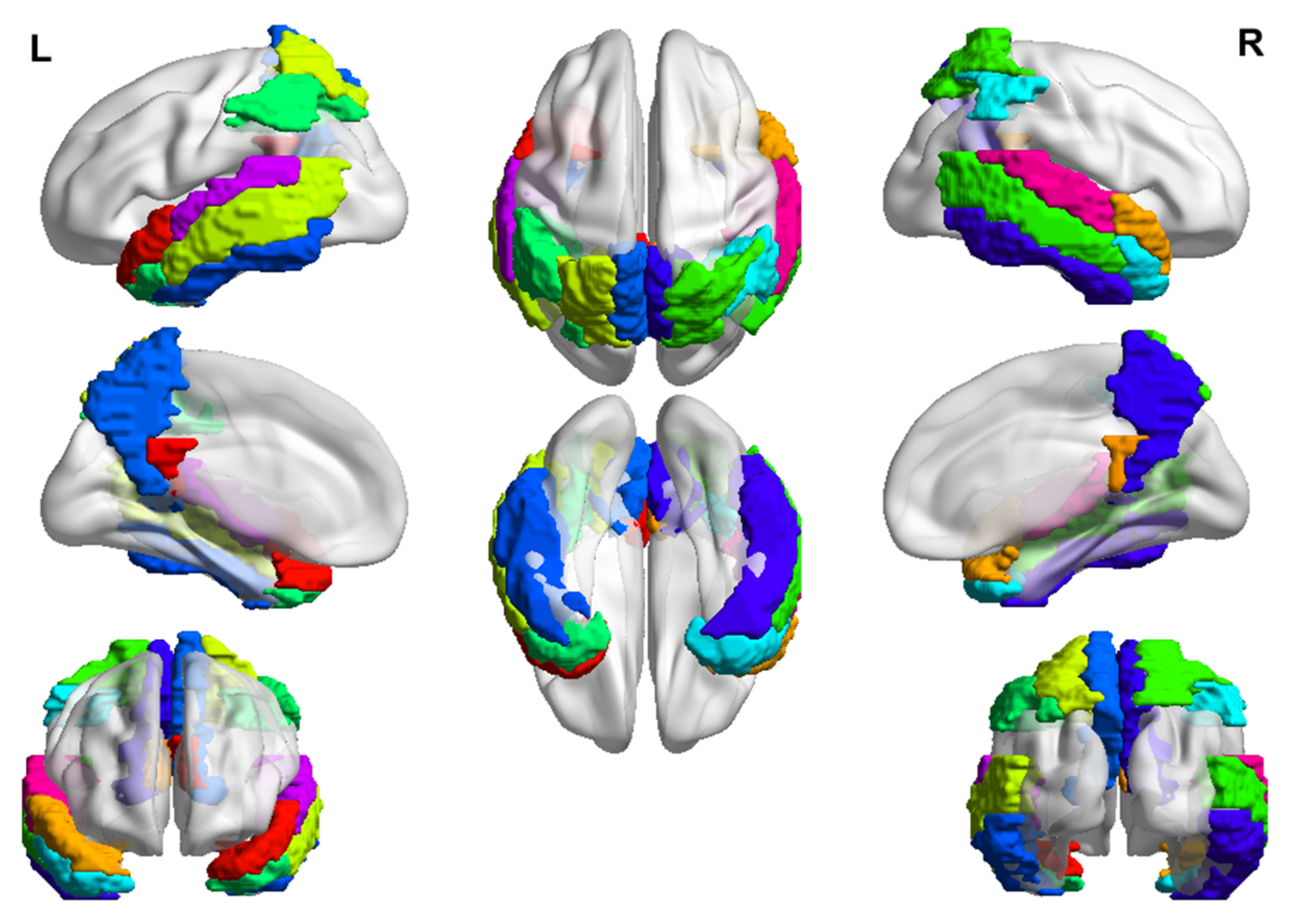
  134. Fan, L.; Li, H.; Zhuo, J.; Zhang, Y.; Wang, J.; Chen, L.; Yang, Z.; Chu, C.; Xie, S.; Laird, A.R.; et al. The Human Brainnetome Atlas: A New Brain Atlas Based on Connectional Architecture. Cereb. Cortex 2016, 26, 3508–3526. [Google Scholar] [CrossRef] [Green Version]
  135. Yakushev, I.; Hammers, A.; Fellgiebel, A.; Schmidtmann, I.; Scheurich, A.; Buchholz, H.-G.; Peters, J.; Bartenstein, P.; Lieb, K.; Schreckenberger, M. SPM-based count normalization provides excellent discrimination of mild Alzheimer’s disease and amnestic mild cognitive impairment from healthy aging. NeuroImage 2009, 44, 43–50. [Google Scholar] [CrossRef]
  136. LeCun, Y.; Bengio, Y.; Hinton, G. Deep learning. Nature 2015, 521, 436–444. [Google Scholar] [CrossRef]
  137. Goodfellow, I.; Bengio, Y.; Courville, A. Deep Learning; MIT Press: Cambridge, MA, USA, 2016. [Google Scholar]
  138. Sharma, S.; Sharma, S.; Athaiya, A. Activation functions in neural networks. Towards Data Sci. 2017, 6, 310–316. [Google Scholar] [CrossRef]
  139. Ruder, S. An overview of gradient descent optimization algorithms. arXiv 2016, arXiv:1609.04747. [Google Scholar]
  140. Medsker, L.R.; Jain, L.C. Recurrent neural networks. Des. Appl. 2001, 5, 64–67. [Google Scholar]
  141. Goodfellow, I.; Pouget-Abadie, J.; Mirza, M.; Xu, B.; Warde-Farley, D.; Ozair, S.; Courville, A.; Bengio, Y. Generative adversarial networks. Commun. ACM 2020, 63, 139–144. [Google Scholar] [CrossRef]
  142. Liu, M.; Cheng, D.; Yan, W.; Alzheimer’s Disease Neuroimaging Initiative. Classification of Alzheimer’s disease by combination of convolutional and recurrent neural networks using FDG-PET images. Front. Neuroinform. 2018, 12, 35. [Google Scholar] [CrossRef] [Green Version]
  143. Ruwanpathirana, G.P.; Williams, R.C.; Masters, C.L.; Rowe, C.C.; Johnston, L.A.; Davey, C.E. Mapping the association between tau-PET and Aβ-amyloid-PET using deep learning. Sci. Rep. 2022, 12, 14797. [Google Scholar] [CrossRef]
  144. Ding, Y.; Sohn, J.H.; Kawczynski, M.G.; Trivedi, H.; Harnish, R.; Jenkins, N.W.; Lituiev, D.; Copeland, T.P.; Aboian, M.S.; Mari Aparici, C.; et al. A deep learning model to predict a diagnosis of Alzheimer disease by using 18F-FDG PET of the brain. Radiology 2019, 290, 456–464. [Google Scholar] [CrossRef]
  145. Guo, J.; Qiu, W.; Li, X.; Zhao, X.; Guo, N.; Li, Q. Predicting Alzheimer’s disease by hierarchical graph convolution from positron emission tomography imaging. In Proceedings of the 2019 IEEE International Conference on Big Data (Big Data), Los Angeles, CA, USA, 9–12 December 2019; pp. 5359–5363. [Google Scholar]
  146. Choi, H.; Jin, K.H.; Alzheimer’s Disease Neuroimaging Initiative. Predicting cognitive decline with deep learning of brain metabolism and amyloid imaging. Behav. Brain Res. 2018, 344, 103–109. [Google Scholar] [CrossRef] [Green Version]
  147. Yee, E.; Popuri, K.; Beg, M.F.; Alzheimer’s Disease Neuroimaging Initiative. Quantifying brain metabolism from FDG-PET images into a probability of Alzheimer’s dementia score. Hum. Brain Mapp. 2020, 41, 5–16. [Google Scholar] [CrossRef] [PubMed]
  148. Pan, X.; Phan, T.L.; Adel, M.; Fossati, C.; Gaidon, T.; Wojak, J.; Guedj, E. Multi-view separable pyramid network for AD prediction at MCI stage by 18 F-FDG brain PET imaging. IEEE Trans. Med. Imaging 2020, 40, 81–92. [Google Scholar] [CrossRef] [PubMed]
  149. Etminani, K.; Soliman, A.; Davidsson, A.; Chang, J.R.; Martínez-Sanchis, B.; Byttner, S.; Camacho, V.; Bauckneht, M.; Stegeran, R.; Ressner, M.; et al. A 3D deep learning model to predict the diagnosis of dementia with Lewy bodies, Alzheimer’s disease, and mild cognitive impairment using brain 18F-FDG PET. Eur. J. Pediatr. 2021, 49, 563–584. [Google Scholar] [CrossRef] [PubMed]
  150. Hojjati, S.H.; Babajani-Feremi, A.; Alzheimer’s Disease Neuroimaging Initiative. Prediction and Modeling of Neuropsychological Scores in Alzheimer’s Disease Using Multimodal Neuroimaging Data and Artificial Neural Networks. Front. Comput. Neurosci. 2021, 15, 769982. [Google Scholar] [CrossRef] [PubMed]
  151. Ryoo, H.G.; Choi, H.; Lee, D.S. Distinct subtypes of spatial brain metabolism patterns in Alzheimer’s disease identified by deep learning based FDG PET clusters. Alzheimer’s Res. Ther. 2021, 13, 49. [Google Scholar] [CrossRef]
  152. Jo, T.; Nho, K.; Risacher, S.L.; Saykin, A.J. Deep learning detection of informative features in tau PET for Alzheimer’s disease classification. BMC Bioinform. 2020, 21, 496. [Google Scholar] [CrossRef]
  153. Bach, S.; Binder, A.; Montavon, G.; Klauschen, F.; Müller, K.R.; Samek, W. On pixel-wise explanations for non-linear classifier decisions by layer-wise relevance propagation. PLoS ONE 2015, 10, e0130140. [Google Scholar] [CrossRef] [Green Version]
  154. Lu, D.; Popuri, K.; Ding, G.W.; Balachandar, R.; Beg, M.F.; Alzheimer’s Disease Neuroimaging Initiative. Multiscale deep neural network-based analysis of FDG-PET images for the early diagnosis of Alzheimer’s disease. Med. Image Anal. 2018, 46, 26–34. [Google Scholar] [CrossRef]
  155. Shen, T.; Jiang, J.; Lu, J.; Wang, M.; Zuo, C.; Yu, Z.; Yan, Z. Predicting Alzheimer disease from mild cognitive impairment with a deep belief network based on 18F-FDG-PET images. Mol. Imaging 2019, 18, 1536012119877285. [Google Scholar] [CrossRef]
  156. Zhang, Z.; Beck, M.W.; Winkler, D.A.; Huang, B.; Sibanda, W.; Goyal, H. Opening the black box of neural networks: Methods for interpreting neural network models in clinical applications. Ann. Transl. Med. 2018, 6, 216. [Google Scholar] [CrossRef]
  157. Selvaraju, R.R.; Cogswell, M.; Das, A.; Vedantam, R.; Parikh, D.; Batra, D. Grad-cam: Visual explanations from deep networks via gradient-based localization. In Proceedings of the IEEE International Conference on Computer Vision, Venice, Italy, 22–29 October 2017; pp. 618–626. [Google Scholar]
  158. Ghazal, T.M.; Issa, G. Alzheimer disease detection empowered with transfer learning. Comput. Mater. Contin. 2022, 70, 5005–5019. [Google Scholar] [CrossRef]
  159. Ashraf, A.; Naz, S.; Shirazi, S.H.; Razzak, I.; Parsad, M. Deep transfer learning for Alzheimer neurological disorder detection. Multimed. Tools Appl. 2021, 80, 30117–30142. [Google Scholar] [CrossRef]
  160. Aderghal, K.; Khvostikov, A.; Krylov, A.; Benois-Pineau, J.; Afdel, K.; Catheline, G. Classification of Alzheimer disease on imaging modalities with deep CNNs using cross-modal transfer learning. In Proceedings of the 2018 IEEE 31st International Symposium on Computer-Based Medical Systems (CBMS), Karlstad, Sweden, 18–21 June 2018; pp. 345–350. [Google Scholar]
  161. Aderghal, K.; Afdel, K.; Benois-Pineau, J.; Catheline, G.; Alzheimer’s Disease Neuroimaging Initiative. Improving Alzheimer’s stage categorization with Convolutional Neural Network using transfer learning and different magnetic resonance imaging modalities. Heliyon 2020, 6, e05652. [Google Scholar] [CrossRef]
  162. Doersch, C. Tutorial on variational autoencoders. arXiv 2016, arXiv:1606.05908. [Google Scholar]
  163. Penning, J.; John, R.; Chandler, H.; Fielding, P.; Marshall, C.; Smith, R. Generative Adversarial Network” Steerability” for Brain PET Image Generation. In Proceedings of the 2021 IEEE Nuclear Science Symposium and Medical Imaging Conference (NSS/MIC), Piscataway, NJ, USA, 16–23 October 2021; pp. 1–4. [Google Scholar]
  164. John, R.; Penning, J.; Chandler, H.; Fielding, P.; Marshall, C.; Smith, R. Quantitative Evaluation of Synthesized Brain PET Using a Variational Autoencoder. In Proceedings of the 2021 IEEE Nuclear Science Symposium and Medical Imaging Conference (NSS/MIC), Piscataway, NJ, USA, 16–23 October 2021; pp. 1–4. [Google Scholar]
  165. Hochreiter, S.; Schmidhuber, J. Long short-term memory. Neural Comput. 1997, 9, 1735–1780. [Google Scholar] [CrossRef]
  166. Srivastava, N.; Hinton, G.; Krizhevsky, A.; Sutskever, I.; Salakhutdinov, R. Dropout: A simple way to prevent neural networks from overfitting. J. Mach. Learn. Res. 2014, 15, 1929–1958. [Google Scholar]
  167. Ioffe, S.; Szegedy, C. Batch normalization: Accelerating deep network training by reducing internal covariate shift. In Proceedings of the International Conference on Machine Learning (PMLR), Lille, France, 6–11 July 2015; pp. 448–456. [Google Scholar]
  168. Wan, L.; Zeiler, M.; Zhang, S.; Le Cun, Y.; Fergus, R. Regularization of neural networks using dropconnect. In Proceedings of the International Conference on Machine Learning (PMLR), Atlanta, GA, USA, 16–21 June 2013; pp. 1058–1066. [Google Scholar]
  169. Lee, C.; Landgrebe, D.A. Decision boundary feature extraction for neural networks. IEEE Trans. Neural Netw. 1997, 8, 75–83. [Google Scholar]
  170. Mao, J.; Jain, A.K. Artificial neural networks for feature extraction and multivariate data projection. IEEE Trans. Neural Netw. 1995, 6, 296–317. [Google Scholar]
  171. Chen, Y.; Jiang, H.; Li, C.; Jia, X.; Ghamisi, P. Deep feature extraction and classification of hyperspectral images based on convolutional neural networks. IEEE Trans. Geosci. Remote Sens. 2016, 54, 6232–6251. [Google Scholar] [CrossRef] [Green Version]
  172. Nixon, M.; Aguado, A. Feature Extraction and Image Processing for Computer Vision; Academic Press: Cambridge, MA, USA, 2019. [Google Scholar]
  173. Egmont-Petersen, M.; de Ridder, D.; Handels, H. Image processing with neural networks—A review. Pattern Recognit. 2002, 35, 2279–2301. [Google Scholar] [CrossRef]
  174. Wachinger, C.; Reuter, M.; Klein, T. DeepNAT: Deep convolutional neural network for segmenting neuroanatomy. NeuroImage 2018, 170, 434–445. [Google Scholar] [CrossRef] [PubMed]
  175. De Brebisson, A.; Montana, G. Deep neural networks for anatomical brain segmentation. In Proceedings of the IEEE Conference on Computer Vision and Pattern Recognition (CVPR) Workshops, Boston, MA, USA, 7–12 June 2015; pp. 20–28. [Google Scholar]
  176. Hunter, C.A.; Kirson, N.Y.; Desai, U.; Cummings, A.K.G.; Faries, D.E.; Birnbaum, H.G. Medical costs of Alzheimer’s disease misdiagnosis among US Medicare beneficiaries. Alzheimer’s Dement. 2015, 11, 887–895. [Google Scholar] [CrossRef] [PubMed] [Green Version]
  177. Petersen, R.C.; Aisen, P.S.; Beckett, L.A.; Donohue, M.C.; Gamst, A.C.; Harvey, D.J.; Jack, C.R., Jr.; Jagust, W.J.; Shaw, L.M.; Toga, A.W.; et al. Alzheimer’s disease neuroimaging initiative (ADNI): Clinical characterization. Neurology 2010, 74, 201–209. [Google Scholar] [CrossRef] [PubMed]
  178. Iwatsubo, T. Japanese Alzheimer’s Disease Neuroimaging Initiative: Present status and future. Alzheimer’s Dement. 2010, 6, 297–299. [Google Scholar] [CrossRef]
  179. Carrillo, M.C.; Bain, L.J.; Frisoni, G.B.; Weiner, M.W. Worldwide Alzheimer’s disease neuroimaging initiative. Alzheimer’s Dement. 2012, 8, 337–342. [Google Scholar] [CrossRef]
  180. Frisoni, G.B. Alzheimer’s disease neuroimaging initiative in Europe. Alzheimer’s Dement. 2010, 6, 280–285. [Google Scholar] [CrossRef]
  181. Cavedo, E.; Redolfi, A.; Angeloni, F.; Babiloni, C.; Lizio, R.; Chiapparini, L.; Bruzzone, M.G.; Aquino, D.; Sabatini, U.; Alesiani, M.; et al. The Italian Alzheimer’s Disease Neuroimaging Initiative (I-ADNI): Validation of Structural MR Imaging. J. Alzheimer’s Dis. 2014, 40, 941–952. [Google Scholar] [CrossRef]
Figure 1. Brain regions that typically show hypometabolism from FDG-PET imaging. Images visualized with BrainNet Viewer [39]. In the top row, we see these areas on the left, top, and right of the outer surface of the brain. In the middle row, we see the left and right medial brain surfaces and the underside of the brain in the center. In the bottom row, we see the anterior and posterior views of the brain. Each color represents a distinct anatomical region of interest.
Applsci 12 11463 g001
Figure 2. Sample output of SPM12. A group-wise comparison was performed on FDG-PET scans of AD patients and healthy controls, and the results were compared by t-testing. Regions of statistically significant differences between the groups ( p = 0.05 with family-wise error adjustment) are shown as dark clusters on the white glass brain. Red arrow points to the global maximum.
Applsci 12 11463 g002
Figure 3. Performing PCA on FDG-PET images reveals disease-specific patterns in AD compared to healthy controls. PCs were obtained and eight of the first 10 were combined via stepwise linear regression to obtain the visualization seen above. Figure shows outer exterior (left) and medial exterior (right) surfaces. Images scaled according to mean z-score and standard deviation of whole images for the purposes of visualization. Reprinted/adapted with permission from Ref. [85]. Copyrights under Creative Commons Attribution 4.0 International License (http://creativecommons.org/licenses/by/4.0/, accessed on 1 October 2022).
Applsci 12 11463 g003
Figure 4. The SVM functions here as a linear binary classifier. The data belonging to either the positive or negative class are plotted, and the optimal boundary between them clearly separates each class. The support vectors used to draw this boundary are centered in a circle of their relevant class color, while examples that violate the slack constraint are circled in black.
Applsci 12 11463 g004
Figure 5. Visualization of the decision boundary for sequential minimal SVM on FDG-PET images of AD patients and healthy controls. Images scaled according to mean z-score and standard deviation of whole images for the purposes of visualization. Reprinted/adapted with permission from Ref. [85]. Copyrights under Creative Commons Attribution 4.0 International License (http://creativecommons.org/licenses/by/4.0/, accessed on 1 October 2022).
Applsci 12 11463 g005
Figure 6. Visualization of feedforward artificial neural network architecture. We have a 16-node input layer followed by two hidden layers of 8 and 4 nodes, respectively. The final layer contains a single output node. At each node, there may be a nonlinear activation function, such as the sigmoid, but each node’s input is the linear combination of connections from the nodes in the preceding layer. Connections between each individual node are visualized: blue edges are negatively weighted, red edges are positively weighted, and edge opacity represents relative magnitude. Weights were initiated randomly for the purpose of visualization. Networks of this type may be used for classification but also for the modeling of highly nonlinear operations.
Applsci 12 11463 g006
Figure 7. Visualization of convolutional neural network architecture specifically designed for classification based on image data. A series of 16@128 × 128 images are input to the network. These frames are passed through a max pooling layer and a convolutional layer before being flattened into a 1D vector. Two fully connected layers of size 256 and 128 connect to a final node containing the network output.
Applsci 12 11463 g007
Table 1. Summary of literature for the identification/classification/prognostication of AD. All studies reporting some combination of sensitivity (SENS), specificity (SPEC), area-under-curve (AUC), or accuracy (ACC) have been considered for inclusion. The use of GLMs is widespread throughout statistical analysis software and programming languages and provides a reliable tool for accounting for the effects of covariates, such as age and sex, with some use as a stand-alone classifier for AD detection. More specialized methods based on the ideas of the GLM, such as 3D-SSP, are engineered for the detection of AD pathology, and progress in research into applying this technique to amyloid and tau imaging is underway. PCA and SSM are both extremely valuable tools for dimensionality reduction (the elimination of unnecessary or redundant data) and the discovery of disease-specific patterns. They are also quite effective prior to classification with an SVM and increase classification accuracy. From the literature surveyed in this review, deep learning-based tools provide the greatest accuracy for differentiating AD patients from healthy controls, differentiating AD from MCI patients, and the clinically relevant task of differentiating pMCI and sMCI patients.
Author/ReferenceMethodologyTaskPerformance
Katako et al. [85]GLMAD vs. HCSENS = 85.6%
SPEC = 86.2%
AUC = 0.922
Ottoy et al. [87]GLMMCI to AD conversionSENS = 92%
SPEC = 96%
Katako et al. [85]PCA/SSM—single PC
PCA/SSM—many PCs
AD vs. HC
AD vs. HC
SENS = 80.2%
SPEC = 78.7%
SENS = 86.5%
SPEC = 81.9%
Teune et al. [114]PCA/SSMAD vs. HCSENS = 93%
SPEC = 94%
Meles et al. [116]PCA/SSMpMCI vs. HCSENS = 82.4%
SPEC = 85.7%
Yokoi et al. [119]PCA/SSMAD vs. HCSENS = 79.1%
SPEC = 82.6%
Perovnik et al. [120]PCA/SSMAD vs. HC
AD vs. MCI & bvFTD
AD vs. DLB
AUC = 0.95
AUC = 0.76–0.85
AUC = 0.87
Katako et al. [85]SVM—ISDAAD vs. HCSENS = 0.84
SPEC = 0.955
AUC = 0.945
Ilan et al. [124]PCA-SVMAD vs. HCSENS = 88.64%
SPEC = 87.70%
ACC = 88.24%
Ramirez et al. [125]SVMAD vs. HCACC = 90.38%
Garali et al. [126]SVMAD vs. HCACC = 95.07%
Damasceno et al. [128]SVMAD vs. MCI vs. non-ADAUC = 0.9
Svaifullah et al. [129]SVMMCI to AD conversionSENS = 81.7%
SPEC = 90.1%
ACC = 87.2%
AUC = 0.94
Ding et al. [130]SVMAD vs. HC
pMCI vs. sMCI
AUC = 0.93
AUC = 0.83
Varatharajah et al. [131]SVM—linear kernelMCI to AD conversionSENS = 93%
SPEC = 77%
ACC = 81%
AUC = 0.93
Zhao et al. [132]SVMsMCI vs. pMCIACC = 89.9%
AUC = 0.892
Liu et al. [141]NN—RNNAD vs. HC
MCI vs. HC
SENS = 91.4%
SPEC = 91%
ACC = 91.2%
AUC = 0.953
SENS = 78.1%
SPEC = 80%
ACC = 78.9%
AUC = 0.839
Ding et al. [143]NN—CNNAD identification
MCI identification
non-AD/non-MCI identification
AUC = 0.93
AUC = 0.63
AUC = 0.73
Guo et al. [144]NN—Graph CNNAD vs. HC
AD vs. MCI vs. HC
ACC = 93%
ACC = 77%
Choi & Jin [145]NN—3D CNNAD vs. HC
pMCI vs. sMCI
ACC = 93%
ACC = 84.2%
Yee et al. [146]NN—Residual CNNAD vs. HC
pMCI vs. sMCI
ACC = 93.5%
AUC = 0.976
ACC = 74.7%
AUC = 0.811
Pan et al. [147]NN—Pyramidal CNNMCI to AD conversionACC = 83.05%
Etmani et al. [148]NN—3D CNNDLB identification
AD identification
MCI identification
AUC = 0.962
AUC = 0.964
AUC = 0.714
Choi et al. [150]NN—3D CNNMCI to AD conversionAUC = 0.89
Jo et al. [152]NN—3D CNNAD vs. HC
MCI vs. HC
SENS = 95.4%
SPEC = 96.9%
ACC = 96.2%
SENS = 48.2%
SPEC = 82.4%
ACC = 64.2%
Lu et al. [154]NN—Multi-scale CNNpMCI vs. sMCIACC = 82.51%
Shen et al. [155]NN—SVM-CNNMCI to AD conversionACC = 86.6%
Publisher’s Note: MDPI stays neutral with regard to jurisdictional claims in published maps and institutional affiliations.

