Updating the FMEA Approach with Mitigation Assessment Capabilities—A Case Study of Aircraft Maintenance Repairs

Abstract

This paper proposes a qualitative model to overcome the limitations of conventional failure mode and effects analysis (FMEA), which does not consider risk mitigation capabilities when prioritizing risks. Failure to consider these capabilities can lead to unrealistic risk estimates, especially when the level of uncertainty is high. In the proposed model, the original applicability of conventional FMEA was retained along with the three conventional risk variables, namely, severity, occurrence, and detectability. In addition, a fourth variable was added to account for risk mitigation capabilities. A case study in the project selection of aircraft repairs was used to demonstrate the implementation of the model and its applicability. The results show that the inclusion of mitigation options leads to more realistic risk scenarios, suggesting that the original FMEA approach may lead to non-conservative risk estimates.

1. Introduction

In a global economy, the competitiveness of companies is a key factor for their sustainable growth. In many cases, competitiveness is based on the anticipation of new businesses, products, and services with a strong innovation component, which is a crucial point for a promising market position [1].

With the goal of quickly bringing competitive offerings to market to gain market positions, many companies struggle to conduct adequate risk analyses, which in many cases has a negative impact, both financially and on brand image. There are numerous examples of this, from the recurring recalls in the automotive industry to the dangers associated with the use of cell phones, where the explosion of the corresponding batteries endangered human lives [2,3,4].

The risk associated with innovation has somewhat slowed down the industry’s in-novation initiatives. This is mainly because risk assessment and management models lack important features needed in practice, such as ease of use, completeness, a low level of theoretical knowledge, and applicability to cases with limited information [5]. The existing models in the literature are either very simple and provide few practical results, or they are very complex and usually developed for specific cases. Therefore, it is necessary to develop risk management tools that correspond to the reality of the company [6].

In fact, innovation is a key factor for the economic growth of companies and organizations and promotes the creation of wealth and social balance. However, a product, an idea, a method, or a service is only innovative if it is proven in practice. In this sense, a high degree of uncertainty is associated with innovation projects and their corresponding products [7].

To circumvent this uncertainty, risk assessment and risk management tools are used to support decision making under uncertainty. These tools can be divided into three categories, namely, quantitative, qualitative, and mixed risk models, which include quantitative and qualitative approaches [8].

The risk method most commonly used in practice in connection with innovations is Failure Modes and Effects Analysis. It is a qualitative method that can be easily adapted to quantitative data as needed. It is easy to learn and apply in practice. Because of these characteristics, it is very popular in a wide range of industries.

It is a method with some limitations, due to the properties of its failure mode prioritization function, called the risk priority number (RPN). There are a number of works in the literature that aim to circumvent these limitations, especially for non-injective and non-surjective problems [9,10,11]. However, at a conceptual level, there is another limitation of FMEA related to the detectability variable used in the RPN function. In its original design, the detectability variable is evaluated qualitatively, while taking into account the existing control methods in the risk scenario. It aims to assess the probability of detecting a particular failure mode before it occurs. However, this approach ignores an important aspect, namely, the ability to mitigate or even eliminate a particular failure mode once it has been detected. To the best of the authors’ knowledge, this issue has never been addressed, although it clearly has implications for failure mode prioritization.

The assessment of risk mitigation capability is not found in the original version of the FMEA model nor in its more recent variants. However, there is a need to develop a methodology that allows FMEA to incorporate the ability to mitigate or eliminate failure modes when they are discovered before they occur. With this in mind, this paper addresses this research question in depth and proposes a new FMEA-based risk model that incorporates the ability to mitigate a particular failure mode into the prioritization of failure modes. In this way, failure modes are ranked not only by their impact, probability of occurrence, and likelihood of detection, but also by the ability of those involved in the risk scenario to mitigate them. Considering this capability when prioritizing failure modes is extremely important, because failure modes with a low RPN resulting from a high detection capacity can become critical failure modes if there is not enough capacity to mitigate or even eliminate them.

Paper Structure

The article consists of seven sections. The introduction provides a comprehensive overview of the research and points out the gaps that led to this research article. Section 2 points out related work in the literature. Section 3 then describes the research methods and introduces the concepts of effective risk and performance variables; Section 4 explains the application of the developed model to a case study. Section 5 describes the results of the case study; Section 6 analyzes the results; and finally, Section 7 draws conclusions from the work conducted.

2. State of the Art

A large number of quantitative risk models can be found in the literature. These models use probabilistic functions and require a considerable amount of data, which makes them unsuitable for the analysis of innovation risks, as little or no data is available in this context [12]. Indeed, the most commonly used risk assessment and management tools rely heavily on quantitative data. This characteristic makes them useless in cases where little or no in-formation is available, as they require access to event logs to obtain stochastic information, which are difficult to obtain in innovation projects. The alternative to overcome this problem is the use of qualitative risk assessment tools that take advantage of the experience of experts to evaluate risk scenarios and corresponding failure modes [13].

However, there are a number of criticisms against these models in the literature. One example is the criticism of models based on FMEA (Failure Modes and Effects Analysis). FMEA is a qualitative risk assessment tool developed by the U.S. Army in the middle of the last century that aims to minimize potential failures in systems, processes, projects, or services [14]. It has been used in a variety of industries and research centers, e.g., NASA [15]. The FMEA approach is suitable for use in design and product development and can be divided into 3 types, namely, functional, design, and process. This framework is simple and easy to implement, which are characteristics that have encouraged its use in recent decades [16].

Despite its popularity, FMEA has some weaknesses that have led to disagreements about its applicability. Most of these disagreements have been caused by the limitations of the risk priority number function (RPN), whose shortcomings in prioritizing failure modes and its dependence on expert experience for its estimates are most often cited in the literature [10,17,18].

Notwithstanding these criticisms, FMEA-based models continue to be widely used in industries because of their applicability and ease of use [19]. However, the results are sometimes ambiguous and require alternative measures to reconcile the results with the logical interpretation of the risk scenario.

Other criticisms of FMEA-based models include the inability to account for relative importance among risk variables; obtaining the same risk index for scenarios with different risks; difficulty in expert evaluation of risk variables; non-injective and non-surjective risk prioritization functions with duplicate values; values that never appear in the risk assessment; scales for assessing risk variables with different paradigms that make it difficult to standardize the contribution of different risk variables; the inability to effectively measure risk reduction after corrective actions; the inability to consider the interdependence of failure modes; and the inability to model the risk of complex scenarios be-cause only three risk variables are considered in these modes, which are not sufficient in certain cases [10].

The models proposed in the literature to overcome these limitations are mostly based on models of multicriteria analysis (AHP, ANP, Fuzzy TOPSIS, DEMATEL, Gray theory) and artificial intelligence (rule-based systems, DEA, Fuzzy DEA). These models are very complex and require prior knowledge of their structures and the underlying theories in each case before they can be used in practice for risk assessment [11,20,21,22,23,24,25].

There are also criticisms of these new models, especially those based on fuzzy theory. The large number of membership functions required by these models calls into question their applicability to real industry cases. In practice, fuzzy theory is often used to over-come consensus and ambiguity problems in the interpretation of expert opinions, but in terms of risk assessment, the level of complexity is high. The maximum number of risk variables considered in these models is still three, although in practice it is necessary to include additional variables, such as cost and impact sub-variables.

Liu et al. [10,26] conducted a remarkable literature review on multicriteria decision making (MCDM) methods that evaluate risks using FMEA. They selected 169 papers from 16 international journals and concluded that many researchers have improved the FMEA approach to overcome the limitations of FMEA by using FMEA together with other MCDM approaches.

The literature review divides the 169 papers into 10 research branches and concludes that it continues to point to the need to include additional risk variables in the traditional FMEA approach. In the original FMEA, only three risk variables are used in the RPN function, namely, severity (S), occurrence (O), and detectability (D). Severity aims to assess the impact of a particular failure mode, occurrence aims to quantify its probability, and detectability aims to quantify the ability to detect a failure mode before it occurs.

However, in many practical cases, additional risk variables are needed to fully characterize risk scenarios. In practice, these additional variables have been conceptually included along with the traditional FMEA risk variables.

For example, assessing the severity of a particular failure mode may involve the impact of several sub-variables, such as: Cost, Profitability, Human, Social, Environmental, etc. If all these sub-variables have the same weight in the risk assessment, their breakdown is not necessary. However, if they contribute with different weight to the risk, which is usually the case, then their breakdown becomes important. In this sense, the original RPN function cannot be used because it considers only three risk variables. This has led to alternative approaches to create new disaggregated severity variables, which in some cases are assessed separately along with their respective occurrence and detectability scores. In this approach, the disaggregated severity variables are scored independently and do not take into account the aggregate interdependence of these variables, which may be a shortcoming in some situations.

Recent studies suggest that the performance of risk assessment and management teams, as well as the resources available for risk management, have a particular influence on the degree of impact of the risk assessment scenario. Despite these findings, there is no systematic methodology in FMEA that takes this aspect into account. This fact mainly results from the limitation to the three variables found in the traditional FMEA. In many cases, a fourth variable, such as risk mitigation performance, is needed.

For example, Alsaidalani et al. [27] developed a risk mitigation model based on FMEA with the aim of improving risk metrics in a hospital’s quality management system. The authors used the traditional RPN together with a detailed description of hospital processes and concluded that it was necessary to integrate risk management programs into quality management programs. In addition to this aspect, the authors also concluded that the performance of process owners had a strong influence on the assessment and management of risks. Despite these conclusions, the proposed risk model did not consider the performance level of process owners to implement mitigation strategies, which was a limitation of the proposed model.

Arrantes et al. [28] proposed a new group decision model based on the FMEA concept combined with ELECTRE TRI and Double Hierarchy Hesitant Fuzzy Linguistic Term Sets (DHHFLTS). The main objective was to evaluate the overall risk of important risk factors that are usually evaluated independently. The authors concluded, among other things, that the complexity of risk mitigation had a strong influence on the classification of failure modes. This conclusion underscores the need for a simple and structured approach to assessing risk mitigation capabilities, which in turn is closely related to the risk owner’s performance in mitigating risk.

Hartanti et al. [29] proposed a framework for identifying waste in higher education institutions that used FMEA, among other tools, to prioritize different categories of waste in scientific research activities. The authors successfully identified the types of waste and prioritized them using the traditional RPN function. The authors pointed out a number of factors that influenced the evaluation and management of waste. Many of these factors were related to the performance of the researcher, so the impact of the identified waste depended on the ability of the individual researcher to address the causes of the waste. In this sense, incorporating each researcher’s performance in reducing or eliminating waste would lead to a more realistic assessment of the impact of waste.

Shafiee et al. [30] proposed a framework that combined FMEA with a hybrid AHP-PROMETHEE approach to prioritize risk mitigation strategies that extend the life of offshore assets. The framework focused on three fronts, namely, the identification, analysis, and assessment of risks associated with oil and gas facilities; the selection of mitigation strategies; and the strategic risk of implementation. The authors concluded that the FMEA model in its traditional form had limitations that prevented its use in prioritizing mitigation strategies, and therefore proposed the AHP-PROMETHEE model as an alternative. While the authors focused on mitigation strategies as a way to mitigate potential impacts, they did not mention anything about the performance of risk managers in terms of their ability to implement these mitigation strategies, which is an important consideration when prioritizing mitigation strategies.

The objective of this work is to develop an FMEA-based model that considers risk mitigation performance in addition to the traditional FMEA variables, i.e., severity, frequency, and detectability, to overcome the limitations identified in practice.

The Problem Tackled

In the original conceptual idea, detectability aimed to quantify the ability to detect a particular failure mode and did not explicitly measure the ability to mitigate that failure mode once it was detected. Therefore, it was traditionally assumed that existing mitigation capabilities were sufficient to minimize or eliminate a failure mode. However, in a given risk scenario, mitigation capabilities may be insufficient or may change due to unexpected events.

Intuitively, these two concepts have been combined in the traditional variable Detectability, which can lead to ambiguous results, i.e., overly conservative or non-conservative risk assessment estimates. As with Severity, which includes multiple sub-variables, Detectability ratings in traditional FMEA are also ambiguous because detection and mitigation are considered together without explicitly assessing mitigation capabilities for a given failure mode and respective risk scenario.

This paper aims to improve the FMEA approach by splitting the traditional risk variable of Detectability in FMEA analysis into Detectability and Mitigation variables. The Mitigation variable aims to remove the ambiguity of traditional Detectability assessments by including mitigation capabilities in the risk assessment. In this way, it becomes possible to improve the effectiveness of the FMEA approach and ultimately improve risk analysis in innovation.

In addition to this goal, a model should be developed that not only improves the prioritization of failure modes, but that also retains the simplicity and ease of use of the traditional FMEA approach to meet the risk assessment and risk management needs that arise in practice.

3. Materials and Methods

This section presents a new qualitative risk assessment model based on the expert evaluation approach to estimate the risk of a given scenario using more than three qualitative risk variables, which is a new contribution to the field of qualitative risk assessment. This model is strongly based on the Failure Mode and Effects Analysis (FMEA) concept, but with some nuances and improvements that allow the extension of the FMEA concept to risk assessment activities with more than three risk variables.

In its original framework, FMEA uses only three risk variables to prioritize failure modes according to their risk. Due to drawbacks, such as the non-injectivity and non-surjectivity of the conventional risk prioritization function (called risk prioritization number—RPN), no risk assessment of failure modes can be performed in the conventional FMEA framework, only their prioritization. To overcome this drawback, the RPI model was developed, which is an injective and surjective qualitative risk model that allows both risk assessment of failure modes and their risk prioritization [9].

In this paper, the RPI model is extended to cover risk scenarios with more than three variables. This feature extends the applicability of the RPI model beyond conventional FMEA risk scenarios and enables risk assessment of failure modes, not just their prioritization. In addition, a performance model, the qualitative performance index (QPI), is proposed along with the RPI extension to set the risk score according to the risk taker’s capabilities to mitigate or avoid failure modes. This proposal allows extrapolation of the concept of failure modes and their risk characterization to non-conventional application scenarios where failure modes may represent undesirable events and their risk characterization allows for risk assessment of such events.

Figure 1 shows the sequence of work developed and presented in this section. First, the RPI model previously developed to overcome the limitations associated with the RPN is described. Then, the proposal to extend the RPI model to include more than three variables (the original RPI model included only three variables) is described and analyzed. Then, the qualitative index to evaluate the mitigation capacity is proposed. Finally, the effective risk model (Erisk) obtained by the extended RPI model is proposed along with the qualitative mitigation index.

3.1. The RPI Model

The risk priority index model [9] was proposed to overcome the problems related to non-injectivity, non-subjectivity, and the lack of weighting in the risk priority function of FMEA. Although the model overcomes the aforementioned problems, it remains with only three risk variables, which limits its applicability. As it stands, it does not allow for the inclusion of a fourth risk variable, i.e., it does not allow for the inclusion of a risk mitigation variable. The RPI model is described by Equation (1):

$$RPI=\left(\frac{w_A{\epsilon }^3+1}{{\epsilon }^3}\right){\delta }_A+\left(\frac{w_B{\epsilon }^2+1}{{\epsilon }^2}\right){\delta }_B+w_C{\delta }_C$$

(1)

where ${\delta }_A,{\delta }_B,{\delta }_C$ are the scale variables of the RPI model, $w_A,w_B,w_C$ are their respective weights depending on the risk scenario, and $\epsilon$ is an injectivity factor, usually equal to 10. The scale variables are calculated using Equation (2) and using the RI function described in Equation (3).

$$\begin{array}{l}{\delta }_A=\frac{RI{\left(A,B,C\right)}_{A>B>C\_rating}+RI{\left(A,B,C\right)}_{A>C>B\_rating}}{2}\\ {\delta }_B=\frac{RI{\left(A,B,C\right)}_{B>A>C\_rating}+RI{\left(A,B,C\right)}_{B>C>A\_rating}}{2}\\ {\delta }_C=\frac{RI{\left(A,B,C\right)}_{C>B>A\_rating}+RI{\left(A,B,C\right)}_{C>B>A\_rating}}{2}\end{array}$$

(2)

Equation (3) shows the general form of the RI function. This function must be set up according to the order of importance of the given risk variables A, B, and C described in Equation (2). In the FMEA analysis, these variables are replaced by S (severity), O (occurrence), and D (detectability).

$$RI{\left(A,B,C\right)}_{A>B>C}=\left(A-1\right)\cdot {\alpha }^2+B\cdot \alpha +C-\alpha$$

(3)

These three variables (A, B and C) can be qualitatively scored on a scale of 1 to 10 for a given failure mode. The typical value of $\alpha$ is 5 or 10, depending on the type of industry. The order of importance of the risk variables is indicated by the subscript in Equation (3), i.e., $A>B>C$; it is a relative and qualitative order of importance of the risk variables. Therefore, the RI function can be set to a different relative importance by changing the position of the risk variables, as shown in Equation (4) for $C>B>A$:

$$RI{\left(A,B,C\right)}_{C>B>A}=\left(C-1\right)\cdot {\alpha }^2+B\cdot \alpha +A-\alpha$$

(4)

3.2. Proposal of a Extended RPI Model

The extension of the RPI model to the risk space with nth variables was done in two steps. First, the RI function was extended to include more than three variables, and then the equations of the scale variables (Equation (2)) were also extended. The RI extension is described in Equation (5), which is an extrapolation of Equation (3) to nth risk variables. Equation (5) retains injectivity and surjectivity and has an output range between 1 and 10. For n = 3, Equation (5) is equivalent to Equation (3).

$$RI{\left(x_1,x_2,\mathrm{\dots },x_n\right)}_{x_1>x_2>\mathrm{\dots }>x_n}={\displaystyle \sum _{i=1}^n\left(x_i-1\right)}\cdot {\alpha }^{n-i}+1$$

(5)

The order of importance of the risk variables is determined by $x_1>x_2>x_3\mathrm{\dots }>x_n$, while $\alpha$ is the scale used to evaluate the risk variables, and $n$ is the dimension of the risk space. For example, in a four-dimensional risk space, Equation (5) is set as follows:

$$RI{(x_1,x_2,x_3,x_4)}_{x_1>x_2>x_3>x_4}=\left(x_1-1\right)\cdot {\alpha }^3+\left(x_2-1\right)\cdot {\alpha }^2+\left(x_3-1\right)\cdot \alpha +\left(x_4-1\right)+1$$

(6)

For a five-dimensional risk space, it is determined as shown in Equation (7):

$$RI{(x_1,x_2,x_3,x_4,x_5)}_{x_1>x_2>x_3>x_4>x_5}=\left(x_1-1\right)\cdot {\alpha }^4+\left(x_2-1\right)\cdot {\alpha }^3+\left(x_3-1\right)\cdot {\alpha }^2+\left(x_4-1\right)\cdot \alpha +\left(x_5-1\right)+1$$

(7)

and so on. The next step is to extend the formulation of the scale variables (Equation (2)) and reduce the scenario risk variables to the same risk scale to account for their combined effect in an nth risk space. They must be determined by considering the permutations of the risk variables, as shown in Equation (2). Thus, for a space with 4 dimensions, there are 4! Permutations (24 permutations), and for a space with 5 dimensions, there are 5! Permutations (120 permutations) and so on. Equation (8) represents 5! possible permutations for a five-dimensional risk space, which corresponds to 120 possible importance orders with five risk variables.

$$\begin{array}{l}a,P(b,c,d,e)\\ b,P(a,c,d,e)\\ c,P(a,b,d,e)\\ d,P(a,b,c,e)\\ e,P(a,b,c,d)\end{array}$$

(8)

Here the function P() stands for permutations without repetition of the risk variables a, b, c, d, and e. Equation (9) represents the extension of Equation (8) to any length of the risk space:

$$\begin{array}{l}{x}_1,P(x_2,x_3,\mathrm{\dots },x_n)\\ x_2,P(x_1,x_3,\mathrm{\dots },x_n)\\ \mathrm{\dots }\\ x_n,P(x_1,x_2,\mathrm{\dots },x_{n-1})\end{array}$$

(9)

where $n$ is the number of risk variables (of the dimension of the risk space).

For simplicity, the first risk variable in each permutation set is called the master risk variable, since its position is maintained for its permutation set. For example, in the set $x_1,P(x_2,x_3\mathrm{\dots }{x}_n)$ of permutations, there are $(n-1)!$ permutations where the first variable is always $x_1$, so $x_1$ is a master risk variable in this set of permutations. So, for each master risk variable there are $(n-1)!$ orders of importance, and for each of these orders of importance, the RI function is evaluated in each failure mode, as shown in Equation (10):

$$R_{ijk}=RI(x_j,P_k(x_1,x_2,\mathrm{\dots },x_n))$$

(10)

where $i$ is the failure mode number, $k$ is the permutation number from 1 to $(n-1)!$, and $j$ is the master risk variable number from 1 to $n$.

Therefore, $R_{ijk}$ is the output value of the extended RI function for failure mode $i$ with respect to master risk variable $j$ and order of importance $k$. For each master risk variable $j$ and order of importance $k$, the failure modes are prioritized according to their respective $R_{ijk}$ values. After these prioritizations, the $R_{ijk}$ values are replaced by their respective rank orders, which are represented as ${\delta }_{ijk}$ from now on. Therefore, the RPI scale variables are calculated as follows:

$${\delta }_{ij}=\frac{{\displaystyle \sum _{k=1}^{(n-1)!}{\delta }_{ijk}}}{n}$$

(11)

The extended risk priority index is given by:

$$RP{I}_i={\displaystyle \sum _{j=1}^{n-1}\left(\frac{w_j\cdot {\epsilon }^{n-j+1}+1}{{\epsilon }^{n-j+1}}\right)\cdot {\delta }_{ij}}+w_n\cdot {\delta }_{in}$$

(12)

where $n$ is the dimension of the risk space. The risk weights $w_j$ determine the order of importance of each risk variable in the risk scenario, and $\epsilon$ is a constant that makes Equation (12) an injective function; in this case $\epsilon =10$.

3.3. Using the Extended RPI to Propose a Qualitative Mitigation Index (QMI)

The risk assessment of a particular failure mode must be performed while considering the possibilities to avoid or mitigate the same failure mode depending on the particular risk scenario and the available resources. In the traditional FMEA, the detectability risk variable aims to correct the critical value resulting from the multiplication of severity and occurrence. However, detectability depends on several factors, such as available resources and knowledge, which may vary depending on the capabilities of the risk owners. Therefore, detectability can be considered as a mitigation-based risk variable that updates the risk level according to the available capabilities to detect failure modes. To illustrate the impact of mitigation performance on risk impact, please consider the following example:

In the last century, the risk of hospital-acquired infections was dramatically reduced when it was discovered that handwashing prevents the spread of disease. So, in this risk scenario, the risk of spreading a particular disease depended heavily on the knowledge that handwashing prevents spread and the ability to put that knowledge into practice. These two cornerstones, knowledge and the ability to put knowledge into practice, can be considered as mitigation variables in this risk scenario that can be used to assess performance in preventing the spread of disease, and thus update the risk level of a given risk scenario.

To extend the concept of risk mitigation variables to generic risk scenarios, reliability, availability, resilience, and robustness are proposed as generic risk mitigation variables to evaluate the performance level of risk mitigation in a given risk scenario. These four risk mitigation variables are generic enough to be applied to any risk scenario, as is the case with the severity, occurrence, and detectability risk variables. Despite their broad scope, they can be easily evaluated in the context of risk scenarios.

There are many definitions of reliability, usually varying by discipline, but all are synonymous with the following: “Reliability is the ability to perform consistently well over an expected period of time”. Thus, to evaluate this risk mitigation variable within a risk scenario with a qualitative approach and using a rating scale of, say, 1 to 10, one can answer the following question based on the resources available and the scope of the risk scenario:

• Do I have the required knowledge, information and experience to perform consistently well and maintain the required level of quality to avoid/mitigate the analyzed failure mode?

This question can be used to assess the ability to do a good job, but not the availability of that ability. In this sense, availability is defined here as a mitigation variable and can be evaluated as an answer to the following question:

• Given the available resources, do I have the necessary human and technical resources to avoid the analyzed failure mode?

In many cases, unexpected events occur that lower the overall level of risk mitigation capability, especially for the reliability and availability mitigation variables. One way to minimize or eliminate their impact is to detect or predict these events before they actually occur. This gives the time needed to make the necessary changes. It is also necessary to consider the time it takes to respond to an identified mitigation performance issue. So, resilience is a variable of mitigation performance that can be used here to measure these concepts, and its rating can be determined by answering the following question:

• Am I able to recover the level of reliability and available performance when adverse events occur and make the necessary changes within an acceptable period of time?

One would think that these three mitigation variables (reliability, availability, and resilience) can be evaluated based on ideal assumptions that are usually taken for granted in the traditional FMEA approach, but this is not true. For example, these performance variables may be negatively impacted by other factors, such as heavy reliance on a particular individual for reliability, or the allocation of human and technical resources to other projects or activities. Therefore, it is important to measure the volatility of the reliability, availability, and resilience scores. For this purpose, a fourth performance variable, robustness, is introduced to correct the performance level according to the expected volatility. To evaluate this variable, the following question must be answered:

• Am I able to maintain the values for reliability, availability, and resilience with the available resources?

Table 1. Questions to rate mitigation variables.

Mitigation Variables	Questions that Support the Ratings Given to Mitigation Variables
Reliability	Do I have the required knowledge, information, and experience to perform consistently well and maintain the required level of quality to avoid/mitigate the analyzed failure mode?
Availability	Given the available resources, do I have the necessary human and technical resources to avoid the analyzed failure mode?
Resilience	Am I able to recover the level of reliability and available performance when adverse events occur and make the necessary changes within an acceptable period of time?
Robustness	Am I able to maintain the values for reliability, availability, and resilience with the available resources?

summarizes the four questions defined for each of the four performance variables. The answers to these questions help to evaluate the performance variables, which can be done using the rating scales shown in Table 1.

These four variables have an orthogonal relationship, i.e., their scope does not overlap, so their classification is mutually exclusive.

Table 2. Mitigation performance ratings, 10-point rating scale.

Reliability	Availability	Resilience	Robustness	Ranking
Absolute Uncertainty	Absolute Uncertainty	Absolute Uncertainty	Absolute Uncertainty	1
Very Remote	Very Remote	Very Remote	Very Remote	2
Remote	Remote	Remote	Remote	3
Very low	Very low	Very low	Very low	4
Low	Low	Low	Low	5
Moderate	Moderate	Moderate	Moderate	6
Moderately High	Moderately High	Moderately High	Moderately High	7
High	High	High	High	8
Very high	Very high	Very high	Very high	9
Almost certain	Almost certain	Almost certain	Almost certain	10

shows a 10-point rating scale for evaluating the performance variables described above on the basis of expert judgments (qualitative evaluation).

In this way, the mitigation performance variables for a given failure mode of a given risk scenario are evaluated according to the experts’ judgments using Table 2.

Then, the qualitative mitigation index (QMI) for a given failure mode is calculated using Equation (13) (extended RPI) by replacing the risk variables with mitigation variables and keeping the calculation process presented in Section 3.2. Equation (13) shows the expression for the QMI.

$$QM{I}_i={\displaystyle \sum _{j=1}^{n-1}\left(\frac{w_j^M\cdot {\epsilon }^{n-j+1}+1}{{\epsilon }^{n-j+1}}\cdot {\delta }_{ij}^M\right)+}{w}_n^M\cdot {\delta }_{in}^M$$

(13)

Here, the index $M$ represents the mitigation variables and their respective weights. Using Equation (13) and considering the four mitigation variables—Reliability, Availability, Resilience, and Robustness, in that order—yields Equation (14), which estimates the degree of mitigation for each failure mode $i$.

$$QM{I}_i=\frac{w_R^M\cdot {\epsilon }^4+1}{{\epsilon }^4}\cdot {\delta }_{iR}^M+\frac{w_A^M\cdot {\epsilon }^3+1}{{\epsilon }^3}\cdot {\delta }_{iA}^M+\frac{w_{\mathrm{Re}}^M\cdot {\epsilon }^2+1}{{\epsilon }^2}\cdot {\delta }_{i\mathrm{Re}}^M+w_{\mathrm{R}o}^M\cdot {\delta }_{i\mathrm{R}o}^M$$

(14)

Here, the weight $w_R>w_A>w_{\mathrm{Re}}>w_{\mathrm{R}o}$ represents the order of importance considered for the mitigation variables in the description of the QMI. However, this order of importance can be changed depending on how the user perceives the mitigation value. Variables ${\delta }_{iR}^M$, ${\delta }_{iA}^M$, ${\delta }_{i\mathrm{Re}}^M$, and ${\delta }_{i\mathrm{R}o}^M$ are the scale variables for mitigation performance calculated using the same procedures described in Section 3.2 for the risk scale variables.

3.4. Updating FMEA Using QMI

In FMEA frameworks, only risk variables are considered to rank failure modes by their RPN number to prioritize failure modes. The focus is only on the failure mode itself. However, the ability to mitigate or eliminate such failure modes is not considered, even though it has a strong influence on the impact of the failure mode. In fact, the RPN number feeds into the detectability risk variable, which measures the probability of detection. This assumes that the available mitigation capabilities are sufficient to reduce or eliminate the effects of the failure mode. However, in some cases, this capability is insufficient, which affects the accuracy of the detectability ratings. Thus, if a failure mode is detected but nothing is done to correct it, it can be concluded that the detectability rating of the RPN number is inadequate. If the RPN number does not account for this problem in the FMEA risk assessment, there may be cases where the RPN underestimates the risk of failure modes.

To overcome this problem, it is proposed to include QMI in the risk assessment procedures to update the impact of the failure mode according to the available mitigation options. In this context, a qualitative risk assessment model (effective risk model) is proposed that balances risk and performance variables to assess the effective risk of a given failure mode within a given scenario. Figure 2 shows the conceptual framework of the proposed qualitative risk model. On the left are the risk variables used in the RPI model and on the right are the four performance variables used in the QMI model described in the previous section.

The effective risk for each failure mode is calculated using Equation (15), where the RPI model expanded to four variables includes three risk variables and mitigation performance:

$$Eris{k}_i=RP{I}_{A>B>C>D}\left(A,B,C,D\right)$$

(15)

where subscript $i$ indicates the failure mode number, and $A,B,C,D$ represent the risk variables S, O, D, and QMI. The order of their importance, $A>B>C>D$, is determined according to the risk scenario paradigm.

QMI is determined using Equation (16) and must be set according to the rating scale defined by range $\left[1:\alpha \right]$, which is also used to evaluate severity, occurrence, and detectability.

Since the mitigation performance has a complementary meaning to the risk, it is necessary to determine the complementary values of the QMI, which are defined by ${\alpha }^4-QP{I}_{\mathrm{mod}el}$. Then, the reduction to scale $\left[1:\alpha \right]$ is done with Equation (16).

$$QM{I}_i=\frac{{\alpha }^4-QM{I}_{i-\mathrm{mod}el}}{{\alpha }^3}$$

(16)

In this way, the effective risk for a given failure mode is calculated by Equation (17).

$$Eris{k}_i=RP{I}_{S>O>QMI>D}\left(S,O,QMI,D\right)$$

(17)

Typically, risk scenarios have more than one failure mode. Therefore, it is useful to evaluate the risk associated with a particular risk scenario, which can be calculated using Equation (18).

$$Eris{k}_{scenario}=\frac{{\displaystyle \sum _{i=1}^{n}Eris{k}_i}}{{\alpha }^4}$$

(18)

In the numerator is the sum of the failure mode risks, where $n$ denotes the number of failure modes. In the denominator is the upper limit of the rating scale used to evaluate the risk variables.

4. Case Study

4.1. Industrial Problem Description

The primary concern of maintenance, repair, and overhaul (MRO) companies is the prevention of Aircraft on the Ground (AOG) events, which negatively impact airlines and MROs, especially in terms of their economic relationships.

AOG events always involve a degree of risk. When they are related to repairs that are not included in the aircraft maintenance manual, the risk of an AOG event increases exponentially because non-standard methods are used to ensure airworthiness, which typically increase repair time.

The need for these repairs began with lifecycle extension programs motivated by developments in the crude oil market, where lower crude oil prices encouraged the return of parked aircraft to airline fleets. These aircraft were fully restored with maintenance programs ranging from structural maintenance to cabin overhauls.

One way to mitigate AOG risk in the case of aircraft repairs not included in maintenance manuals is to design and develop these aircraft repairs. MRO companies can be certified to develop these types of repairs, but several issues have been raised, primarily because these types of activities are not part of the MROs’ core business.

One of these issues is the long time required to develop repairs, which in some cases can take up to 2 years. This delay is usually due to the fact that there are not enough staff for development, and technical resources are limited.

In order to perform development activities in repairs design, MRO companies need what is known as a Design Organization Approval Certificate (DOA), which is issued by regulatory agencies such as the FAA or EASA. This certificate allows not only the development of new repairs, but also the development of Supplemental Type Certificate (STC) projects, i.e., major changes to an existing type-certificated aircraft, i.e., major changes to the original design. In many cases, these changes bring enormous economic benefits.

Therefore, it is useful to evaluate the ability of a particular MRO to perform the mechanical design activities of aircraft repairs. The evaluation of MRO performance in mechanical design can be quantified by assessing the risk that the design activities will not be performed well on a particular project. This assessment brings several benefits, such as the ability to create project portfolios and optimize resource allocation (technical and human).

To develop new repairs or changes to the original design of an aircraft, MROs must overcome a number of mechanical design challenges. The first and biggest challenge is the lack of information about the original design. The original design is proprietary and not available outside of OEMs. Typically, MROs start from scratch on this type of project without OEM support. As a result, MROs know nothing about the materials, surface treatments, bonding technology and its curing parameters, and other design variables used in the OEM’s original design.

Another limitation is the human resources available for design. Typically, the skills required for maintenance are quite different than those required for design. As a result, maintenance personnel tend to be more technically oriented than scientifically oriented, which can lead to a lack of design knowledge and experience.

In addition, the lack of scientifically oriented personnel can lead to a heavy reliance on a small number of experts, which can lead to a number of management limitations. In addition, maintenance and design activities are typically performed by the same staff, so design activities tend to take second place, which negatively impacts productivity and encourages project delays.

Another limitation is the lack of required technologies in MRO hangars. In many cases, different kinds of technologies are needed for repairs than for building a component from scratch. MRO companies are struggling to survive economically, due to airline requirements and demands, so they rarely invest in technologies that are not used in their core business. This fact severely limits design activities.

In this context, this case study focuses on the case of a Portuguese commercial aircraft that was faced with the need to perform repairs that were not described in the aircraft’s maintenance manual. These repairs have been systematically identified for the Airbus A320 family, especially for aircraft older than 20 years. Currently, the repairs are being carried out by a third-party company to restore the airworthiness of the damaged components, which has a huge economic and logistical impact on this company.

This company has the DOA certificate to perform design activities, but does not have a structured approach to evaluate its ability to perform these activities. Therefore, the extended RPI model proposed in this paper is used to access this capability so that the company can make informed decisions about its project portfolio and its investment in human and technical resources.

4.2. Aircraft Failures Requiring Repair Development

This section describes three repairs that the company had to send to a third-party company because the aircraft maintenance manual did not provide instructions on how to perform the repairs. This had a negative impact on the company. If the company had developed repair instructions for these defects, it would have achieved significant benefits for the company.

4.2.1. Corrosion in Aircraft Turbofan Intakes

A corrosion defect that frequently occurs on the turbine intakes of the A320 is not mentioned in the original equipment manufacturer’s (OEM) maintenance manual. This defect occurs in the contact area between the intake acoustic panels and the titanium mounting ring. Figure 3 shows the geometry of the Airbus A320 inlet and the corrosion defect.

The inner inlet of the intake consists of three acoustic panels made of aluminum sandwich structures attached to a titanium ring with retaining ring screws (see Figure 3b).

Figure 4 shows a typical corrosion pattern found in A320 inlets. This corrosion results from a galvanic corrosion process between a titanium ring and an aluminum doubler (aluminum sheet). The formation of the galvanic dielectric is caused by the formation of microcracks in the adhesive, due to aging of the adhesive and high stresses in the adhesive layer. These stresses are favored by thermal loads and by different coefficients of thermal expansion of the different materials in the adhesive joint, which can increase local stresses to values close to the shear strength of the adhesive joint.

Titanium and aluminum have different coefficients of thermal expansion, so they are subjected to different contraction stresses at low temperatures. For this reason, relative contraction occurs at the interface between the different materials, resulting in different strain levels and creating interface stresses. These stresses are the same as those experienced by the adhesive, since its job is to bond the two surfaces without slippage.

4.2.2. Failure of Bonding in Fan Cowl Doors

Another maintenance event without maintenance procedures involves the fan cowl doors in the nacelle of the A320 aircraft. The fan cowl doors are frequently opened during turbofan engine maintenance to access the hydraulic systems and to check fluid levels (see Figure 5). During this maintenance work, the fan cowl doors remain open with the aid of two struts. However, it is common for the fan cowl doors to fall down due to incorrect locking at the end of the struts.

The fan cowl doors are made of composite materials held together with adhesives. The impact caused by the fan cowl doors falling down and/or denting often causes the composite materials to peel off. The aircraft maintenance manual provides instructions for repairing delamination at specific locations on the fan cowl doors, but there are no repair instructions for other locations. Figure 6 shows a picture of a fan cowl door that was found to be delaminated and for which there were no instructions from the original manufacturer for this damage.

4.2.3. Corrosion Failure of a Thrust Reverser Pivoting Door Actuator Fitting

Figure 7a shows the pivoting door operation in the deployed state. These doors are open during the aircraft landing to assist the braking system. During braking, they are exposed to aggressive gasses, rain, and ice, which promote corrosion, especially in some aluminum alloys. Figure 7b shows a detail of a swing door, with an aluminum fitting indicated by a white arrow.

In the original aircraft design, the fitting material is made of Duralumin 2024-T4, which has excellent fatigue properties, but very poor resistance to corrosion. As a result, there have been several reports of these fittings being replaced due to corrosion problems.

The fittings replacements have been regularly undertaken with negative economic impact to airliners, with huge benefits expected from replacing the old 2024 aluminum alloy with a newer 6000 or 7000 series aluminum alloy that has better mechanical properties.

4.3. Risk Scenario Definition

Usually, design activities follow a framework to define the main tasks in design, production, and quality control. The goal is to address the main challenges of the project during design and production in an efficient way. The waterfall model or the V-model are two well-known models that are widely used in the development of new products and services. In these models, the very first phase is user requirements elicitation, an important task that involves evaluating sensitive information to understand customer wants and needs. An incorrect assessment of user requirements in a given project will lead to additional resource consumption and consequently to unexpected costs.

In the context of aircraft repair design and production, it is important to understand and evaluate the ability to perform a particular project, especially the ability to correctly identify requirements. This approach helps to understand MRO performance in design, development, and production for the project in question, and provides insights that can support management decisions.

The topic of requirements elicitation is the subject of research in a variety of academic fields, from management to product design and development [31,32,33].

Because of the greater importance of user requirements elicitation, and because of its impact on project delays or abandonment, this research focuses on this topic in the context of developing the repairs already described in Section 4.2. In this context, the extended RPI model is used to assess the risk of failure modes in user requirements elicitation in each of the three repair projects.

To understand the causes that lead to problems in eliciting user requirements, Donald Firesmith [34,35,36] conducted a study that identified and described the main problems in eliciting user requirements. The results of this study are summarized in

Table 3. Most common failure modes found in requirements identification process [34,35,36].

FM	Failure Mode	Failure Causes	Failure Effects
1	Poor requirements quality	Inadequate access to stakeholders and other sources of requirements.	Increased development and sustainment costs; major schedule overruns.
2	Use of inappropriate constraints	Specification of unnecessary requirements	Prevents a better solution to the problem from being selected.
3	Requirements not traced	Requirements are not documented, difficulty in tracing large numbers of requirements	The impact of proposed and actual changes in requirements is not known
4	Missing requirements	Significant requirements are accidentally overlooked	Difficult and expensive to include the missing requirements.
5	Uncontrolled requirements change	Excessive requirements volatility and unmanaged scope creep	Havoc with existing architectures, designs, implementations, and testing.
6	Inadequate verification of requirements quality	Failure to verify sufficiently early in the development process whether the requirements have sufficient quality or not	Requirements defects that are not identified during the requirements engineering process negatively impact all subsequent activities.
7	Inadequate requirements management	Requirements stored in different media and by different teams without interconnection and feedback	Scattered requirements are hard to find, sort, query, and maintain.
8	Inadequate requirements process	Requirements method used is largely undocumented. It is often incomplete in terms of either missing or inadequately documented important tasks, techniques, roles, and work products.	Inconsistently specified requirements, which are difficult for architects, designers, implementers, and testers to use.
9	Inadequate tool support	Lack of support tools, no use or inadequate use of support tools.	Increase in inconsistencies; documented requirements easily get out-of-date.
10	Unprepared requirements engineers	Lack of specific technical experience and training	Inability to understand and follow good requirements methods; production of poor requirements.

from a FMEA perspective, where each problem is considered as a failure mode (column 1) with a description of its causes and effects (columns 2 and 3, respectively).

From now on, the ten failure modes described in Table 3 will be considered here as the main causes of failure in user requirements elicitation and management, and are used in this case study to assess the risk of inadequate user identification in aircraft repair projects.

This type of information is particularly important in portfolio selection, where evaluating business performance against a particular project is an important process in the go-no-go decision process for project selection.

Qualitative Evaluation of the Failure Modes in the Elicitation of User Requirements

In this section, the failure modes described in Table 3 are qualitatively assessed for each of the three repairs described in Section 4.2. The qualitative variables of severity, occurrence, detectability, reliability, availability, resilience, and robustness are used and rated using the 10-point scale described in Table 2. These ratings were obtained through interviews with MRO experts and entered in

Table 4. Inlet corrosion repair project—risk and performance ratings using a 10-point scale.

FM	Severity	Occurrence	Detectability	Reliability	Availability	Resilience	Robustness
1	8	6	6	6	4	4	2
2	5	4	6	5	4	4	3
3	6	6	5	7	4	4	3
4	7	3	1	4	4	3	5
5	3	3	1	5	4	4	5
6	9	5	5	6	4	4	5
7	8	3	6	7	4	3	5
8	7	3	2	5	4	5	5
9	8	6	2	2	2	5	8
10	9	5	2	2	2	5	8

,

Table 5. Fan cowl doors repair project—risk and performance ratings using a 10-point scale.

FM	Severity	Occurrence	Detectability	Reliability	Availability	Resilience	Robustness
1	7	3	1	3	5	4	3
2	5	3	4	7	5	4	4
3	6	5	4	7	6	4	4
4	5	3	1	3	5	4	4
5	7	6	1	5	6	4	4
6	8	4	4	5	4	4	3
7	7	4	6	7	6	4	4
8	7	5	1	7	6	4	4
9	8	4	1	2	3	2	5
10	9	4	1	2	3	2	5

and

Table 6. Fitting corrosion repair project—risk and performance ratings using a 10-point scale.

FM	Severity	Occurrence	Detectability	Reliability	Availability	Resilience	Robustness
1	8	4	1	8	4	4	5
2	5	3	2	7	4	5	5
3	6	3	3	6	4	4	5
4	7	3	3	5	4	4	5
5	6	4	3	5	4	4	5
6	6	4	2	8	4	4	5
7	5	2	2	8	4	4	5
8	8	2	2	7	4	4	5
9	8	2	2	8	4	2	8
10	8	2	2	6	4	2	8

. The experts selected for this type of interviews needed to have extensive experience in the field and a thorough knowledge (technical and human) of the capabilities and limitations of the company that would carry out the project. In situations where it was not possible to obtain statistical information about each risk variable, as in the case study presented, these experts used a scale from 1 to 10 to assign the value of each variable based on their experience and knowledge, as is the case with the traditional FMEA method.

At this point, it was assumed that the values reported in Table 4, Table 5 and Table 6 actually reflected the actual state of the MRO for each of the seven variables in each of the three design projects. The authors were aware of the possible subjectivity of qualitative assessments and that there are tools and methods to overcome this subjectivity, but this issue is beyond the scope of this study. However, if qualitative data are available for each of the seven variables, the correlation between the quantitative data and the 10-point scale described in Table 4, Table 5 and Table 6 can be easily established.

5. Results

For simplicity, the projects to repair corrosion in the turbofan engine intakes, delamination in the fan cowl doors, and corrosion in the thrust reverser actuator fitting were henceforth referred to as Project 1, Project 2, and Project 3, respectively. The following results were obtained considering the following approach:

• Evaluate the original RPI model for each project with weights 0.4, 0.3, and 0.3 for Severity, Occurrence, and Detectability, respectively.
• Evaluate the proposed QMI with weights 0.4, 0.3, 0.2, and 0.1 for Reliability, Availability, Robustness, and Resilience, respectively.
• Evaluate the extended RPI model with the QMI (Effective risk—Erisk), considering three cases with the different weights of each risk variable.
• Consider a lower and upper bound for the risk in each project.

5.1. Evaluation the Original RPI Model for Each Project

Table 7. RPI results for the three design projects considered in this study and weights S 0.4, O 0.3 and D 0.3.

FM	Project 1 RPI	Project 2 RPI	Project 3 RPI
1	655	334	413
2	452	349	281
3	534	464	358
4	334	247	402
5	160	441	394
6	628	515	360
7	547	539	245
8	368	406	375
9	519	413	375
10	526	457	375

shows the RPI values for each failure mode described in Table 3 for each project. The results were obtained using Equation (12) and considering the following weights: 40% for severity, 30% for occurrence, and 30% for detectability. The maximum value in the risk scale is 1000, which results from the number of risk variables considered in the risk scenario, which in this case is three.

From Table 7, it can be concluded that Project 1 had the highest risk of not performing well in user requirements elicitation, followed by Project 2, and ranked last was Project 3. These results do not account for the ability to avoid or overcome failure modes after detection. To capture this capability, the QMI model described in Section 3 was used.

5.2. QMI Evaluation for Each Project

The qualitative scores for the QMI variables are described in Table 4, Table 5 and Table 6, in columns 4 through 7. The weights for each risk mitigation performance variable were 40% for reliability, 30% for availability, 20% for robustness, and 10% for resilience.

Table 8. QMI results for the three design projects considered in this study.

FM	Project 1 QMI	Project 2 QMI	Project 3 QMI
1	6.38	7.22	5.20
2	6.67	5.45	5.41
3	5.85	5.18	6.03
4	7.06	7.10	6.44
5	6.44	6.00	6.44
6	6.03	6.67	5.20
7	5.82	5.18	5.20
8	6.23	5.18	5.61
9	7.68	8.36	5.26
10	7.68	8.36	6.09

shows the QMI results for each failure mode and project. First, the QMI for each failure mode was scored on a scale of 1 to ${\alpha }^4$, where $\alpha =10$. The results were scaled down to a 10-point scale by dividing the QMI results by ${\alpha }^2$. The QMI results for each failure mode were then scaled down to a 10-point scale. This downscaling allows the performance score to be placed on the scale used to evaluate the risk variables in the risk scenarios considered in this study.

The performance ratings obtained for each project were considered along with the severity, occurrence, and detectability risk variables. Therefore, columns 4 through 7 of Table 4, Table 5 and Table 6 were replaced with the corresponding values in Table 8.

The effective risk of each failure mode was evaluated using Equation (17), and the weights are described in

Table 9. Effective risk evaluation—weights given to the risk variables, Cases 1 to 3.

Risk Variables	Project 1	Project 2	Project 3
QMI	0.3	0.3	0.2
Severity	0.3	0.4	0.1
Occurrence	0.2	0.2	0.4
Detectability	0.2	0.1	0.3

.

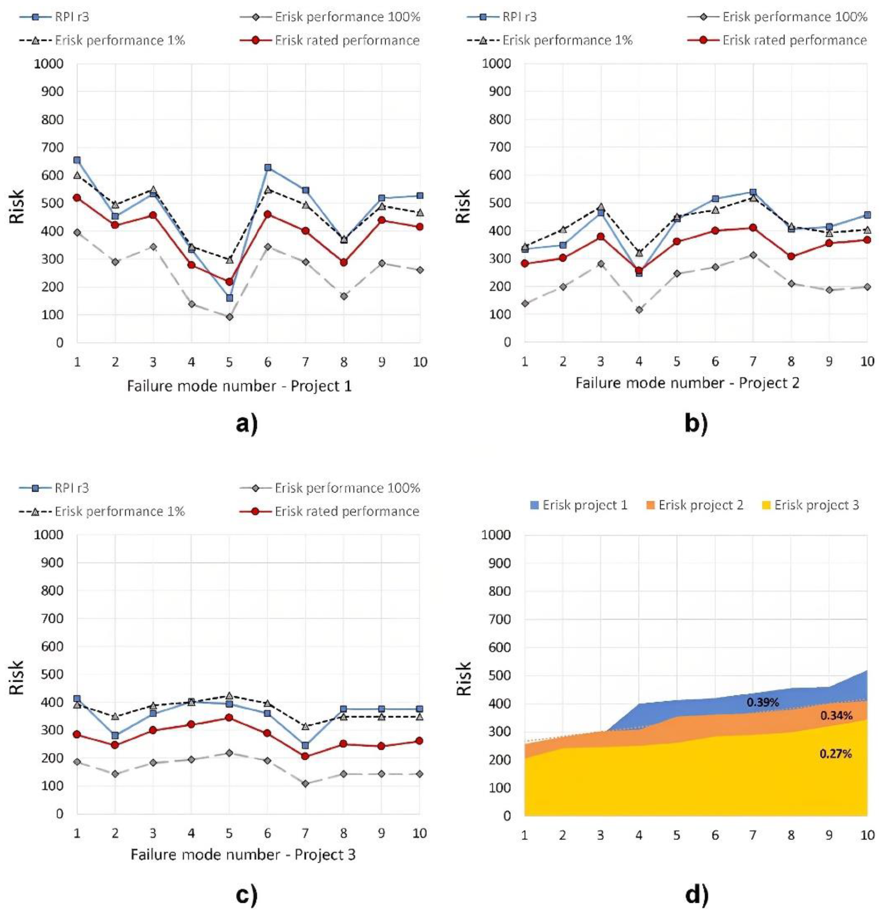
5.3. Extended RPI Assessment (Erisk) for Each Project and Three Weighting Scenarios

Case 1 describes a risk scenario in which severity and QMI have equal weight to occurrence and detectability. This is the case, severity (SxO) has a moderate impact, as do detectability and mitigation. Case 2 describes a risk scenario in which severity plays a major role, followed by QMI; these types of risk scenarios are associated with safety issues. Finally, Case 3 describes a risk scenario where quality control is an issue. An example of this is mass production, where the number of rejected items can have a strong impact on production costs. Depending on the risk scenario and the respective criteria, these weightings can be determined using the Analytic Hierarchy Process (AHP) method or another similar method.

Figure 8, Figure 9 and Figure 10 show the results for effective risk (Erisk) in cases 1, 2, and 3, as described in Table 9. Subfigures (a), (b), and (c) show the risk score for each failure mode, and sub-figure (d) shows the effective risk for each project.

In each sub-figure (a), (b), and (c), four risk scenarios are described for the 10 failure modes considered. The first scenario is RPI r3, indicated by a square. In this scenario, no mitigation variables were considered, i.e., it represents the traditional RPI model where risk is assessed in a risk space with 3 variables (S, O, D).

The second risk scenario considered the Erisk model, where the QMI was taken into account. This scenario is indicated by a circle marker and was evaluated in a risk space with 4 variables (S, O, QMI, D).

Sub-figure (d) shows the effective risk (Erisk) assessed for each project. The results were obtained by calculating the area under each Erisk result obtained for each failure mode previously ranked in ascending order. This order does not affect the results, but it does improve the comparison between the effective risk of each project. Therefore, the values on the x-axis of sub-figure (d) have no practical meaning, i.e., they are not associated with a particular failure mode, as is the case for sub-figures (a), (b), and (c).

The lower and upper bounds, represented by a diamond and a triangle, were obtained by setting the QMI for the lower bound to 1% and for the upper bound to 100% for each failure mode.

6. Discussion

In Cases 1 and 2, all failure modes had a risk value (RPI r3) that was within the risk limit defined by performance at 1% and 100%, and the upper and lower risk limits were calculated considering the QMI weight of 30% in the risk value.

This result was consistent with the hypothesis that the QMI performance model could increase or decrease the risk level compared with the results obtained using only the RPI model, i.e., risk assessment without considering performance.

This feature can be seen in the overlap of the square and circular lines in Cases 1 and 2. For example, in failure mode 3, the RPI r3 result was higher than the Erisk result, which meant that the performance model reduced the risk level in this failure mode, due to the performance capabilities. In failure mode 4, on the other hand, the opposite was true. When the performance score in the equation was included, the risk level for this failure mode increased, due to the low performance capabilities.

However, in Case 3, without the risk-mitigating performance capabilities, the risk value for some failure modes was higher than the 1% upper bound defined by the risk-mitigating performance capabilities. This result was due to an inconsistency between the risk scenarios. The weighting of RPI r3 was unchanged in all three cases; the weighting was 40% for severity, 30% for occurrence, and 30% for detectability. However, the weighting for the assessment of actual risk in Case 3 was 20% for the QMI, 10% for severity, 40% for occurrence, and 30% for detectability. Therefore, the reported weights modulated two different risk scenarios, leading to some inconsistencies.

Moreover, it was difficult to achieve full compatibility between risk scenarios with different risk dimensions because the distribution of weights among risk variables could not be done in the same way, since the number of risk variables changed with the dimension of the risk scenario. In the case of RPI r3, only three variables were considered, so the risk scenario had three weights, and in the case of Erisk, four variables were considered, resulting in a risk scenario with four weights. Therefore, it was necessary to choose the right weights to compare risk scenarios with different risk dimensions. In order to perform such a comparison, the risk scenario paradigm had to be maintained.

The correlation between Cases 1 and 2 showed a slight increase in the effective risk of Case 2, due to a 10% increase in severity. Due to the scale used, this is not very clear in the graphs, but one can easily come to this conclusion when analyzing the data. In addition, the risk level in Case 3 generally decreased for all failure modes except failure mode number 5, which was the result of the lower weighting given to this case in terms of severity and QMI, as well as the lower score given to the risk variables in this project. Thus, the results of the effective risk model were sensitive to the variation of the inputs, and their variations had a significance that was in line with expectations.

Table 10. Effective risk (ER) results for the three design projects considered in this study.

Case 1
	Erisk rated	Lower limit	Delta
Project 1	0.48	0.29	0.18
Project 2	0.43	0.26	0.18
Project 3	0.38	0.22	0.16
Case 2
	Erisk rated	Lower limit	Delta
Project 1	0.50	0.32	0.18
Project 2	0.46	0.29	0.17
Project 3	0.41	0.25	0.16
Case 3
	Erisk rated	Lower limit	Delta
Project 1	0.39	0.26	0.13
Project 2	0.34	0.22	0.12
Project 3	0.27	0.17	0.10

shows the summary of the results for Projects 1 to 3 and Cases 1 to 3. The second column shows the Erisk of the projects considering the 10 failure modes; these results can be seen in the subframes (d) of Figure 8, Figure 9 and Figure 10. In the third column, the projects with a lower Erisk were found by evaluating the area below the lines defined by the diamond marking in the subframes (a), (b), and (c) of Figure 8, Figure 9 and Figure 10. Finally, in the fourth column, the difference was found between the actual Erisk results and the minimum possible Erisk results.

In all cases, Project 1 was the one with the highest Erisk, followed by Project 2, and the least risky was Project 3. This means that it was riskier for the Portuguese MRO to determine the user requirements in Project 1 than in Projects 2 and 3. Therefore, special attention must be paid to this project to avoid delays and unexpected problems.

The delta results in the fourth column of Table 10 show the risk mitigation that can be done to optimize risk by improving performance. These results showed that projects with higher Erisk scores also had higher scores for the scale variables. This is evident when you compare the Erisk and scale variable results for Cases 1 and 3. Typically, projects with higher risk also have higher economic returns. So, if you know how to reduce risk by improving risk mitigation, this could be a way to improve economic returns and competitiveness.

6.1. Practical and Theoretical Implications

6.1.1. Practical Implications

It can be concluded that the extension of the RPI model to risk dimensions greater than three was successfully performed, which allowed the inclusion of an additional risk variable in the FMEA analysis.

The innovative approach of the proposed model is to split the detectability variable from the traditional FMEA model into two components. One component relates to the degree of ability to detect failure modes, and the other component relates to the degree of ability to mitigate failure modes. In this way, the proposed model allows the FMEA-like analysis to consider not only the ability to detect, but also the ability to mitigate. The conventional FMEA approach does not explicitly consider the ability to mitigate, i.e., it assumes that it is always possible to mitigate or eliminate a particular failure mode once it is detected. This may not be the case at the beginning of the project or at some point during project implementation.

In this sense, the proposed model of FMEA analysis allows the inclusion of the mitigation capabilities of the stakeholders in the risk scenario under study, making the risk analysis closer to the reality. In addition to this feature, the proposed model also allows for the creation of a range of outcomes, the boundaries of which are defined by a QPI of 1% (minimum or zero performance) and a QPI of 100% (maximum performance). This information is extremely important for decision making when making investments to improve mitigation capacity and/or eliminate outages. In addition to this aspect, this outcome boundary also allows for the identification of the available scope for mitigation improvements that actually impact the risk associated with the scenario under study.

Furthermore, the model developed can be applied to any type of project, since any type of project can go wrong. Typically, projects are divided into tasks that depend on technical and human requirements that may be missing or whose performance may vary over time. By analyzing these requirements, it is possible to identify failure modes that impact performance and find ways to mitigate these failure modes. With this information and the application of the proposed model, it is possible to identify the critical failure modes associated with the project and thus implement risk management measures to address the potential causes of performance degradation.

6.1.2. Theoretical Implications

Although the main objectives of this study were largely satisfactorily achieved, it was not possible to develop the proposed model with the same simplicity and ease of use as the original FMEA model. The addition of a fourth dimension (four risk variables) to the risk dimension significantly increased the complexity of the risk assessment, which in turn required a more cumbersome computational approach. In this sense, and in order to implement the proposed model, it was necessary to run a programming script to calculate the risk associated with a given scenario. This was not very practical to be implemented by non-programmers in an Excel spreadsheet, as is the case with the model of the traditional FMEA, where no programming skills are required to implement the model. See the Appendix A for the MATLAB script developed for the case study analyzed in this paper.

However, this limitation can be seen as an opportunity to improve the experience of potential users of the proposed model through the development of Excel macros that allow the adaptation of the model to the risk dimension of the scenario under study, as well as the automatic execution of all calculations inherent to the model. In this way, possible negative effects in the use of the proposed model resulting from its complexity can be mitigated.

7. Conclusions

In this work, the RPI model, originally developed with only three risk variables, was extended to risk spaces with more than three variables, a property that allows FMEA-based users to qualitatively evaluate more complex risk scenarios. The original properties, such as injectivity and surjectivity, were retained.

In addition, a qualitative mitigation performance index (QMI) was developed to account for four performance variables. This model allowed for fine-tuning of the risk assessment by considering the available mitigation capabilities and updating the detectability ratings to the actual capabilities of the risk partner. The detectability ratings only assessed the ability to detect failure modes, not the ability to mitigate them. The QPI performance model addressed this shortcoming.

An effective risk model (Erisk) was developed by entering severity, occurrence, detectability, and the QMI performance variable, which is the output of the qualitative performance model, together. This effective risk may be higher or lower than the risk assessed without the performance variables, i.e., lower performance may have increased the risk assessed only with severity, occurrence, and detectability. On the other hand, a higher performance value may have decreased this risk.

The QMI performance risk variable allowed for defining the concept of available risk reduction, i.e., the difference between the actual effective risk and the risk calculated at 100% performance. This risk margin helped to understand whether the allocation of resources to improve performance was appropriate or not.

The models developed were applied to a case study where risk was assessed in the first stage of the V-model. This stage is what is known as user requirements elicitation, which has a major impact on the success of product design and development. In the risk scenario, user requirements were modulated with ten failure modes that were qualitatively assessed for the three projects in the case study.

The risk of failure in determining user requirements was assessed for the three projects and the higher risk project, Project 1, was identified. The risk margin for each project was also assessed. It was found that for these projects, the higher the risk, the higher the risk margin. If the higher risk project has a greater economic impact, which is usually the case, reducing the risk margin by improving performance will reduce project risk and consequently increase the likelihood of project success.

Moreover, the results also showed that the proposed model was sensitive to variations in the mitigation performance. This means that the total risk of the scenario calculated by the proposed model varied depending on the mitigation capabilities, which was an expected result, while in the original RPI model could not take this property into account, so its estimates may become unrealistic, as well as the estimates of the original FMEA approach. In this sense, the proposed model improved the FMEA analysis by allowing for the inclusion in the analysis of the mitigation options available in the scenario under study.

Limitations and Future Works

The main limitation of the work developed in this study were its complexity and difficult implementation without good programming skills. The goal of developing a model that overcomes the limitations of FMEA while maintaining its simplicity was not achieved. Future work is planned to reduce the complexity of the model and develop an Excel macro to improve the usability of the proposed model.

References

1. Dyllick, T. Environment and Competitiveness of Companies. In International Environmental Management Benchmarks; Springer: Berlin/Heidelberg, Germany, 1999; pp. 55–69. [Google Scholar]
2. Wang, Y.-Y.; Wang, T.; Calantone, R. The Effect of Competitive Actions and Social Media Perceptions on Offline Car Sales after Automobile Recalls. Int. J. Inf. Manag. 2021, 56, 102257. [Google Scholar] [CrossRef]
3. Mankowski, P.J.; Kanevsky, J.; Bakirtzian, P.; Cugno, S. Cellular Phone Collateral Damage: A Review of Burns Associated with Lithium Battery Powered Mobile Devices. Burns 2016, 42, e61–e64. [Google Scholar] [CrossRef]
4. Ahsan, K. Trend Analysis of Car Recalls: Evidence from the US Market. Int. J. Manag. Value Supply Chain. 2013, 4, 1. [Google Scholar] [CrossRef]
5. Vargas-Hernández, J.G. Modeling Risk and Innovation Management. J. Compet. Stud. 2011, 19, 45. [Google Scholar]
6. Henschel, T. Risk Management Practices of SMEs: Evaluating and Implementing Effective Risk Management Systems; Erich Schmidt Verlag GmbH & Co. KG: Berlin, Germany, 2008; Volume 68. [Google Scholar]
7. Bilbao-Osorio, B.; Rodríguez-Pose, A. From R&D to Innovation and Economic Growth in the EU. Growth Change 2004, 35, 434–455. [Google Scholar]
8. Haimes, Y.Y. Risk Modeling, Assessment, and Management; John Wiley & Sons: Hoboken, NJ, USA, 2005. [Google Scholar]
9. Anes, V.; Henriques, E.; Freitas, M.; Reis, L. A New Risk Prioritization Model for Failure Mode and Effects Analysis. Qual. Reliab. Eng. Int. 2018, 34, 516–528. [Google Scholar] [CrossRef]
10. Liu, H.-C.; Liu, L.; Liu, N. Risk Evaluation Approaches in Failure Mode and Effects Analysis: A Literature Review. Expert Syst. Appl. 2013, 40, 828–838. [Google Scholar] [CrossRef]
11. Liu, H.-C.; Wang, L.-E.; Li, Z.; Hu, Y.-P. Improving Risk Evaluation in FMEA with Cloud Model and Hierarchical TOPSIS Method. IEEE Trans. Fuzzy Syst. 2018, 27, 84–95. [Google Scholar] [CrossRef]
12. Panjer, H.H. Operational Risk: Modeling Analytics; John Wiley & Sons: Hoboken, NJ, USA, 2006. [Google Scholar]
13. Krause, P.; Fox, J.; Judson, P.; Patel, M. Qualitative Risk Assessment Fulfils a Need. Appl. Uncertain. Form. 1998, 1455, 138–156. [Google Scholar]
14. Lipol, L.S.; Haq, J. Risk Analysis Method: FMEA/FMECA in the Organizations. Int. J. Basic Appl. Sci. 2011, 11, 74–82. [Google Scholar]
15. Reid, R.D. FMEA—Something Old, Something New. Qual. Prog. 2005, 38, 90–93. [Google Scholar]
16. Mikulak, R.J.; McDermott, R.; Beauregard, M. The Basics of FMEA.; CRC Press: Boca Raton, FL, USA, 2017. [Google Scholar]
17. Kutlu, A.C.; Ekmekçioğlu, M. Fuzzy Failure Modes and Effects Analysis by Using Fuzzy TOPSIS-Based Fuzzy AHP. Expert Syst. Appl. 2012, 39, 61–67. [Google Scholar] [CrossRef]
18. Karim, M.A.; Smith, A.J.R.; Halgamuge, S. Empirical Relationships between Some Manufacturing Practices and Performance. Int. J. Prod. Res. 2008, 46, 3583–3613. [Google Scholar] [CrossRef]
19. Wu, Z.; Liu, W.; Nie, W. Literature Review and Prospect of the Development and Application of FMEA in Manufacturing Industry. Int. J. Adv. Manuf. Technol. 2021, 112, 1409–1436. [Google Scholar] [CrossRef]
20. Ishak, A.; Siregar, K.; Naibaho, H. Quality Control with Six Sigma DMAIC and Grey Failure Mode Effect Anaysis (FMEA): A Review. In Proceedings of the IOP Conference Series: Materials Science and Engineering, Kazimierz Dolny, Poland, 21–23 November 2019; IOP Publishing: Bristol, UK, 2019; Volume 505, p. 012057. Available online: https://iopscience.iop.org/article/10.1088/1757-899X/505/1/012057 (accessed on 25 September 2022).
21. Kumar, M.B.; Parameshwaran, R. A Comprehensive Model to Prioritise Lean Tools for Manufacturing Industries: A Fuzzy FMEA, AHP and QFD-Based Approach. Int. J. Serv. Oper. Manag. 2020, 37, 170–196. [Google Scholar] [CrossRef]
22. Jahangoshai Rezaee, M.; Yousefi, S.; Eshkevari, M.; Valipour, M.; Saberi, M. Risk Analysis of Health, Safety and Environment in Chemical Industry Integrating Linguistic FMEA, Fuzzy Inference System and Fuzzy DEA. Stoch. Environ. Res. Risk Assess. 2020, 34, 201–218. [Google Scholar] [CrossRef]
23. Li, J.; Chignell, M. FMEA-AI: AI Fairness Impact Assessment Using Failure Mode and Effects Analysis. AI Ethics 2022, 2, 837–850. [Google Scholar] [CrossRef]
24. Pourmehdi, M.; Paydar, M.M.; Asadi-Gangraj, E. Reaching Sustainability through Collection Center Selection Considering Risk: Using the Integration of Fuzzy ANP-TOPSIS and FMEA. Soft Comput. 2021, 25, 10885–10899. [Google Scholar] [CrossRef]
25. Bujna, M.; Kotus, M.; Matušeková, E. Using the DEMATEL Model for the FMEA Risk Analysis. Syst. Saf. Hum. Tech. Facil. Environ. 2019, 1, 550–557. [Google Scholar] [CrossRef] [Green Version]
26. Liu, H.-C.; Chen, X.-Q.; Duan, C.-Y.; Wang, Y.-M. Failure Mode and Effect Analysis Using Multi-Criteria Decision Making Methods: A Systematic Literature Review. Comput. Ind. Eng. 2019, 135, 881–897. [Google Scholar] [CrossRef]
27. Alsaidalani, R.; Elmadhoun, B. Quality Risk Management in Pharmaceutical Manufacturing Operations: Case Study for Sterile Product Filling and Final Product Handling Stage. Sustainability 2022, 14, 9618. [Google Scholar] [CrossRef]
28. Arantes, R.F.M.; Calache, L.D.D.R.; Zanon, L.G.; Osiro, L.; Carpinetti, L.C.R. A Fuzzy Multicriteria Group Decision Approach for Classification of Failure Modes in a Hospital’s Operating Room. Expert Syst. Appl. 2022, 207, 117990. [Google Scholar] [CrossRef]
29. Hartanti, L.P.S.; Gunawan, I.; Mulyana, I.J.; Herwinarso, H. Identification of Waste Based on Lean Principles as the Way towards Sustainability of a Higher Education Institution: A Case Study from Indonesia. Sustainability 2022, 14, 4348. [Google Scholar] [CrossRef]
30. Shafiee, M.; Animah, I. An Integrated FMEA and MCDA Based Risk Management Approach to Support Life Extension of Subsea Facilities in High-Pressure–High-Temperature (HPHT) Conditions. J. Mar. Eng. Technol. 2022, 21, 189–204. [Google Scholar] [CrossRef]
31. Fernandes, J.; Henriques, E.; Silva, A.; Moss, M.A. Requirements Change in Complex Technical Systems: An Empirical Study of Root Causes. Res. Eng. Des. 2015, 26, 37–55. [Google Scholar] [CrossRef]
32. Aldave, A.; Vara, J.M.; Granada, D.; Marcos, E. Leveraging Creativity in Requirements Elicitation within Agile Software Development: A Systematic Literature Review. J. Syst. Softw. 2019, 157, 110396. [Google Scholar] [CrossRef] [Green Version]
33. Coughlan, J.; Macredie, R.D. Effective Communication in Requirements Elicitation: A Comparison of Methodologies. Requir. Eng. 2002, 7, 47–60. [Google Scholar] [CrossRef]
34. Firesmith, D. Prioritizing Requirements. J. Object Technol. 2004, 3, 35–48. [Google Scholar] [CrossRef] [Green Version]
35. Firesmith, D. Specifying Good Requirements. J. Object Technol. 2003, 2, 77–87. [Google Scholar] [CrossRef] [Green Version]
36. Firesmith, D. Common Requirements Problems, Their Negative Consequences, and the Industry Best Practices to Help Solve Them. J. Object Technol. 2007, 6, 17–33. [Google Scholar] [CrossRef] [Green Version]
Figure 1. Materials and methods framework followed in this research.
Applsci 12 11407 g001
Figure 2. Effective risk model framework.
Applsci 12 11407 g002
Figure 3. A320 intake (a) geometry and assembly (b) inner barrel panel.
Applsci 12 11407 g003
Figure 4. A320 intake (a) corrosion pattern, (b) aluminum corrosion detail.
Applsci 12 11407 g004
Figure 5. A320 fan cowl doors and support struts.
Applsci 12 11407 g005
Figure 6. A320 fan cowl door damage identification spots. The repair procedures for these damages cannot be found in the aircraft maintenance manual.
Applsci 12 11407 g006
Figure 7. (a) Pivoting door operation, (b) pivoting door detail.
Applsci 12 11407 g007
Figure 8. Case 1, risk results considering the weights QMI 0.3, Severity 0.3, Occurrence 0.2, Detectability 0.2 (a) project 1 results, (b) project 2 results, (c) project 3 results, (d) effective risk for projects 1, 2, and 3 considering the weights of Case 1.
Applsci 12 11407 g008
Figure 9. Case 2, risk results considering the weights QMI 0.30, Severity 0.4, Occurrence 0.2, Detectability 0.1. (a) project 1 results, (b) project 2 results, (c) project 3 results, (d) effective risk for projects 1, 2, and 3 considering the weights of Case 2.
Applsci 12 11407 g009
Figure 10. Case 3, risk results considering the weights QMI 0.2, Severity 0.1, Occurrence 0.4, Detectability 0.3. (a) project 1 results, (b) project 2 results, (c) project 3 results, (d) effective risk for projects 1, 2, and 3 considering the weights of Case 3.
Applsci 12 11407 g010