Article

Integrating Different Scales into Species Distribution Models: A Case for Evaluating the Risk of Plant Invasion in Chinese Protected Areas under Climate Change

1
College of Agriculture and Animal Husbandry, Qinghai University, Xining 810016, China
2
State Key Laboratory of Plateau Ecology and Agriculture, Qinghai University, Xining 810016, China
*
Author to whom correspondence should be addressed.
Appl. Sci. 2022, 12(21), 11108; https://doi.org/10.3390/app122111108
Submission received: 8 September 2022 / Revised: 27 October 2022 / Accepted: 31 October 2022 / Published: 2 November 2022

Abstract

:
Species distribution models (SDMs) based on fine-scale environmental data may reduce the uncertainty in predicting species distributions. However, many scientists have also projected the robust potential distributions of species using environmental data of different scales and found that the potential distributions modeled using SDMs are scale dependent. This may be due to the impact of the scale effect on species richness (as well as on multi-species distributions). To eliminate the impact of the scale effect, we aim to develop an improved method to integrate different scales into species distribution models. We use protected areas as the study regions and propose the hypothesis that there is a spatial element to the threat of invasive species for protected areas under climate change. We use Maxent to compute the current and future invasion ability and invasion inequality of invasive species for protected areas based on the potential distributions of species across different scales to evaluate the risk of invasive species. We find that an increase in the number of present records could reduce the accuracy of SDMs. There is a significant linear relationship between the fine-scale and coarse-scale risk of invasive species of alien plants in protected areas, and an appropriate scale should thus be selected to assess species risk based on this linear relationship of invasive risk. There is a significant relationship between the potential of IAPS to invade protected areas and the invasion inequality of IAPS in protected areas across all scales, and 5.0 arcminutes is the most appreciate scale to evaluate the risk of IAPS for protected areas under climate change based on principal component analysis. We provide new insights into the use of species distribution models coupled with different spatial scales to analyze the regional risks associated with species and to assess regional biodiversity.

1. Introduction

Species distribution models (SDMs) are widely used to predict current and future species distributions under various climatic models [1,2,3]. For instance, we can use the results of modeling to develop actionable recommendations for biological conservation and risk prevention and control [4,5,6]. Despite their important uses, there are still many technical issues involved with the use of SDMs [7,8]. Addressing these issues will greatly improve the forecasting accuracy of SDMs, improve the feasibility of environmental management/policymaking, and create a bridge between modelers and decision-makers.
A significant challenge is due to the fact that using SDMs to predict the current and future potential distributions of species gives different results at different resolution scales [9,10,11]. For instance, some climate refugia modeled at fine scales might be missed at coarser scales and reducing uncertainty in estimates of richness may improve the accuracy of modeling at fine scales [3,11,12]. However, a false sense of the accuracy of future climate scenarios might result in unreliable SDMs when using fine scales [13,14], and some studies have used coarse resolutions to determine the robust potential distributions of species around the world [4,5,12,15]. Moreover, climate factors are the best predictor of species richness at the finer scales of resolution because of the spatial scale effect [16]. Therefore, we aimed to put forward a solution to address the contradiction between the fine scale and the coarse scale and to balance results from different scales to develop robust distribution models [17,18].
There is usually a linear relationship between fine scales and coarse scales in terms of the model outputs of SDMs [9,17,19]. Therefore, the results of SDMs can be balanced with different ecological interpretations based on different scales using multivariate statistics. For example, principal component analysis (PCA) offers the possibility to promptly generate results, integrating different data with linear regression [20,21]. PCA is a statistical approach based on actual needs, from which several smaller aggregate variables are chosen, and reflects the information of the original variables as much as possible. PCA can be used to compact redundant data into fewer non-correlated and independent dimensions that are often more readily interpretable than the source data [20]. The linear relationship of SDM offers an opportunity to balance the various results across different spatial scales and then select an appropriate scale that is representative of all scales for further analysis, such as the prediction of the potential species distribution, risk assessments concerning invasive species, and the planning of priority protected areas [17,18,22,23]. We therefore used a statistical approach to find solutions to determine the various potential distributions of species at different scales and used the appropriate scale to produce robust distribution models. Our method is meaningful for planning long-term management decisions to model the habitat quality of species across different spatial scales.
Here, we developed a method to balance the various results based on different scales and used the appropriate scale to model the potential distributions of species. To show how our approach works, we considered the case of the invasion of invasive alien plant species (IAPS) into protected areas in mainland China. We used Maxent to model the current and future potential distributions of nine IAPS at different spatial scales in protected areas in the mainland of China (the scale range of grid resolutions was 2.5–30.0 arcminutes) and quantified the potential IAPS-invaded protected areas and the inequalities related to the invasion of protected areas by IAPS. We showed that our approach is better able to integrate different scales into species distribution models. Our approach can use different scales to project the potential distributions of species. Our results clearly showed the impact of scales on the results of SDMs and showed that SDMs are more practical for decision-making in regard to management policies.

2. Materials and Methods

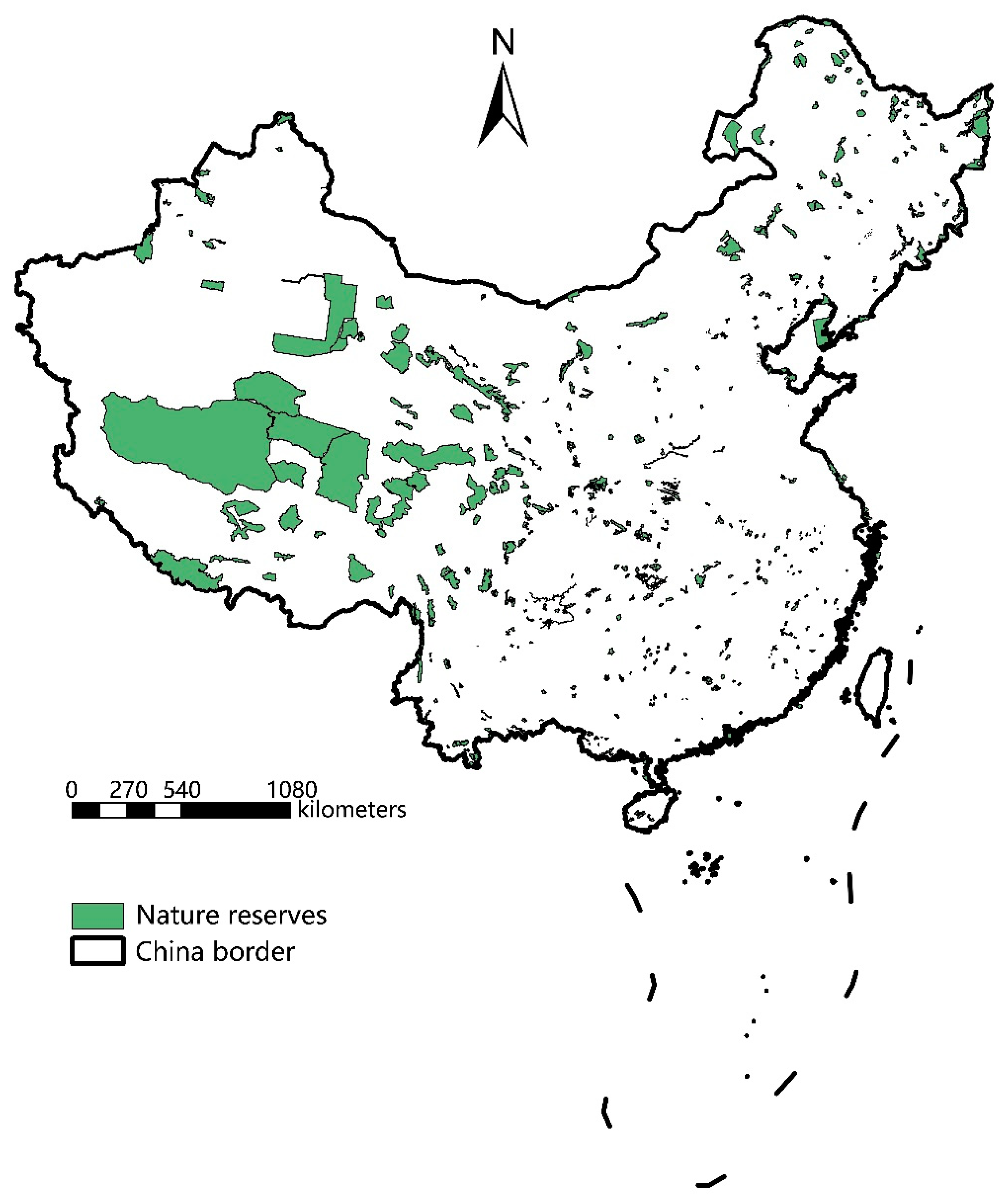
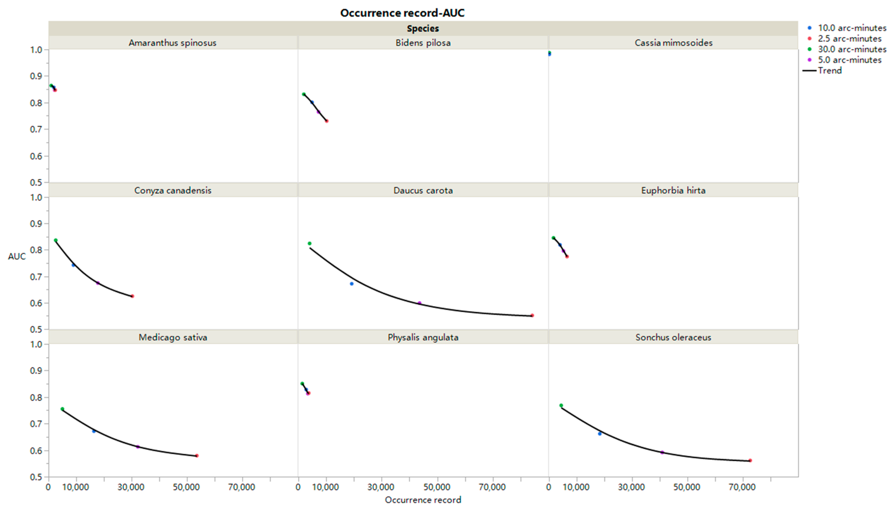
2.1. Data on Species and Protected Areas

We selected nine IAPS with widespread distributions in China from the list of “100 of the World’s Worst Invasive Alien Species” compiled by the Invasive Species Specialist Group (www.issg.org). We selected species according to two criteria: (1) the species had significantly invaded mainland China and (2) there were more than 25 occurrence records that ensured the reliability of the SDMs [8,24]. These species included Amaranthus spinosus, Bidens pilosa, Chamaecrista mimosoides, Erigeron canadensis, Daucus carota, Sonchus oleraceus, Physalis angulata, Euphorbia hirta, and Medicago sativa. The occurrence records of the nine IAPS, especially the specimens or recorded sightings, were compiled from various online databases, including the Global Biodiversity Information Facility (GBIF; www.gbif.org (accessed on 17 September 2020)) and the Chinese Virtual Herbarium (CVH; www.cvh.org.cn (accessed on 1 August 2014); Table S1; [5]). The location descriptions we used were provided in CVH and the literature for the determination of locations in Google Earth and ArcGIS 10.2 ([15]; ESRl, 2014). We used 425 protected areas to evaluate the regional risk of IAPS at different spatial scales, as listed in Table S2. The data on protected areas were downloaded from the Resource and Environmental Science and Data Center (https://www.resdc.cn/Default.aspx (accessed on 5 December 2021)), as shown in Figure 1.

2.2. Environmental Data

We modeled current and future potential distributions of IAPS in protected areas using eight bioclimatic variables, namely the annual mean temperature, annual precipitation, temperature seasonality, mean diurnal range, mean temperature of the wettest quarter, mean temperature of the warmest quarter, precipitation of the driest month, and precipitation seasonality (averages from 1950 to 2000; www.worldclim.org (accessed on 1 August 2014)), which were downloaded from the WorldClim database. We selected two greenhouse gas concentration scenarios (mohc_hadgem2_es RCP 4.5 and 8.5) from global climate models to simulate the future potential distributions of IAPS in the 2080s (2071–2099; http//www.ccafs-climate.org (accessed on 1 August 2014)). RCP 4.5 differs from RCP 8.5 in that RCP 8.5 has higher cumulative concentrations of carbon dioxide than RCP 4.5. Thus, it predicts different climates caused by various anthropogenic concentrations of greenhouse gases and other pollutants. RCP 8.5 and RCP 4.5 were used as the high- and low-concentration scenarios, respectively (www.ccafs-climate.org). Here, we used four resolution scales of bioclimatic variables (2.5, 5.0, 10.0, and 30.0 arcminutes) as the gradient spatial scales because these resolutions are typically used in SDMs.
The distribution of IAPS is determined not only by climatic factors but also by the presence of suitable patches for colonization and establishment. Habitat invisibility can depend on topography, soil characteristics, land cover, and the disturbance regime. Hence, we downloaded four soil variables with a spatial resolution of 5 min (~10 km), including soil pH in H2O and KCl solutions, bulk density (kg m−3), cation exchange capacity (cmol+/kg), and soil clay (wt%) of fine soil fraction (<2 mm) from a study by Hengl et al. [25]. Agricultural land (cropland and pasture area) data for the year 2000, as an indicator of land cover and land use, was downloaded from EarthStat (http//www.earthstat.org/ (accessed on 10 July 2022)) with a spatial resolution of 5 min (~10 km). These data show the proportion of farmland and pasture area (i.e., a fraction of the 5-arcminute grid cell area) quantifying the satellite-derived land cover data and agricultural inventory data [8]. Elevation data (2.5, 5.0, 10.0, and 30.0 arcminutes) were downloaded from the WorldClim database (www.worldclim.org). The data on agricultural lands and the soil variables were resampled to 2.5, 5.0, 10.0, and 30.0 arcminutes, the same as the climate and elevation variables.

2.3. Species Distribution Models (SDMs)

Maxent (version 3.3.3k; http://www.cs.princeton.edu/~schapire/maxent/ (accessed on 10 July 2022)) was used to model the current and future potential distributions of the nine IAPS based on the native and invasive ranges around the world at four spatial scales (2.5, 5.0, 10.0, and 30.0 arcminute resolutions). Maxent was used to estimate the latent distribution functions for nine IAPS based on the maximum entropy and then modeled their geographic locations based on environmental variables. In maps predicted using Maxent, cells with a value of 1 have the highest distribution probability, and those with a value of 0 have the lowest. Furthermore, potential distribution areas were determined in relation to the areas where climate conditions of the study region were similar to the sites where occurrence localities were already recorded [8,26]. In this way, the computed result reflected the possibility of potential distributions used to evaluate the risk of IAPS for protected areas [18,27].
Four-arcminute-resolution current and future climate variables were used as environmental input layers for current and future data in Maxent. To improve the accuracy of Maxent, a 10-fold cross-validation method was used to divide the present dataset into 10 roughly equal partitions, nine of which were used to train the model, and the 10th of which was used to generate SDM estimates [8]. The regularization multiplier (beta) was set to 2.0 to produce a smooth and general response [28]. The maximum number of background points was 10,000 using automatic features; other values remained defaults. We used the jackknife method to test the importance of bioclimatic variables [1,26].
The receiver operating characteristic (ROC) curve uses each value of the predicted outcome as a possible judgment threshold. We used the area under the ROC curve (AUC) to evaluate the performance of the Maxent model. When the randomly selected background points were removed from the dataset, this statistic treats each estimate as a possible threshold based on the corresponding sensitivity and specificity. The SDMs predicted the possibility of potential distribution of invasive species with high accuracy. A higher AUC indicates a better performance by the SDM [1,19,26].

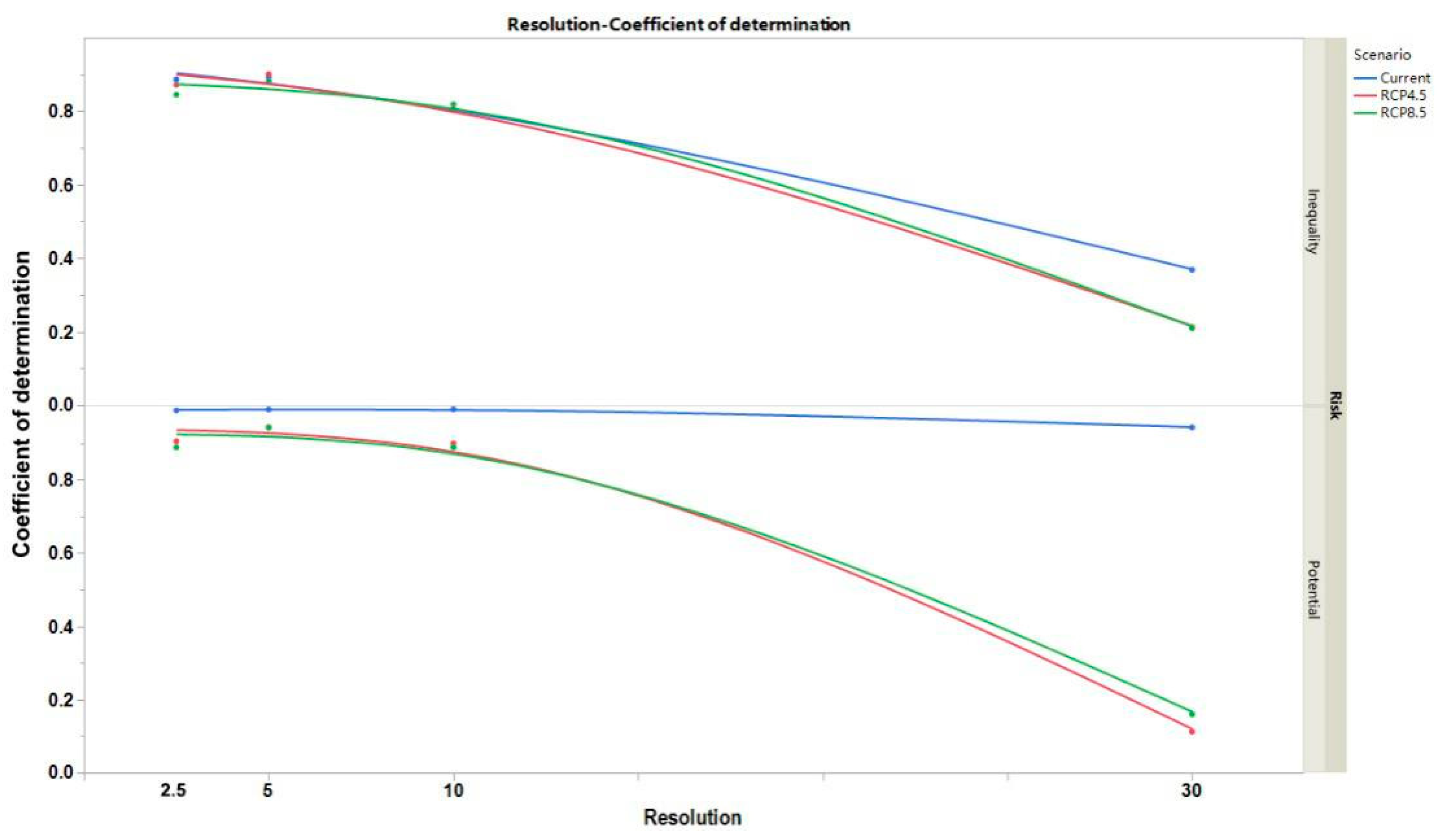
2.4. Evaluating the Risk of IAPS for Protected Areas

We evaluated the risk of IAPS for protected areas based on multiple species because (1) we needed to have enough replicates to test the effects of spatial scales on the potential distribution of IAPS to determine our analysis’s representativeness; (2) there is co-occurrence of IAPS within conservation habitats in one of the most comprehensive global conservation management databases (the Nature Conservancy’s conservation projects) [29]; and (3) IAPS may invade different vegetation types, e.g., deserts, swamps, grasslands, subtropical evergreen broad-leaved forests, monsoon forests, and warm-temperate deciduous broad-leaved forests, and thus the risk of IAPS could be assessed for protected areas with full coverage of vegetation types.
We defined two indicators to evaluate the risk of IAPS for protected areas: (1) the potential of IAPS to invade protected areas and (2) the invasion inequality of IAPS for protected areas. The former indicator was used to assess the risk of IAPS for the overall protected area, and the latter was used to assess the differentiation of the grids of protected areas. Here, we mainly applied the risk of IAPS for the overall protected area in the case of our study.
We used the improved method of Calabrese et al. [30] to evaluate the current and future likelihood of the underlying distribution of IAPS in each pixel:
E j = k = 1 k P i , k
where Ej represents the possibility of potential distribution of IAPS in each pixel j, k is the number of species in pixel j, i is the species i, and Pi,k is the probability of an appropriate potential distribution for species i in pixel j.
We also computed the potential of IAPS to invade each protected area as follows [4]:
S t = j = 1 n X j Y j
where St is the potential of IAPS to invade protected area t, n is the total number of IAPS, Xj is an indicator of the possibility of a species’ potential distribution (Ej value) in grid j of protected area t, and Yj is the distribution area percentage of grid j in protected area t.
Additionally, we calculated the standard deviation of the current and future possibility of species potential distribution in each protected area to assess the discrete degree of IAPS distribution, namely, the inequality of the IAPS risk for each protected area, as follows:
D t = S T D ( E j )
where Dt represents the inequality of IAPS invasion for protected area t and Ej represents the possibility of the potential distribution of IAPS in each pixel j.

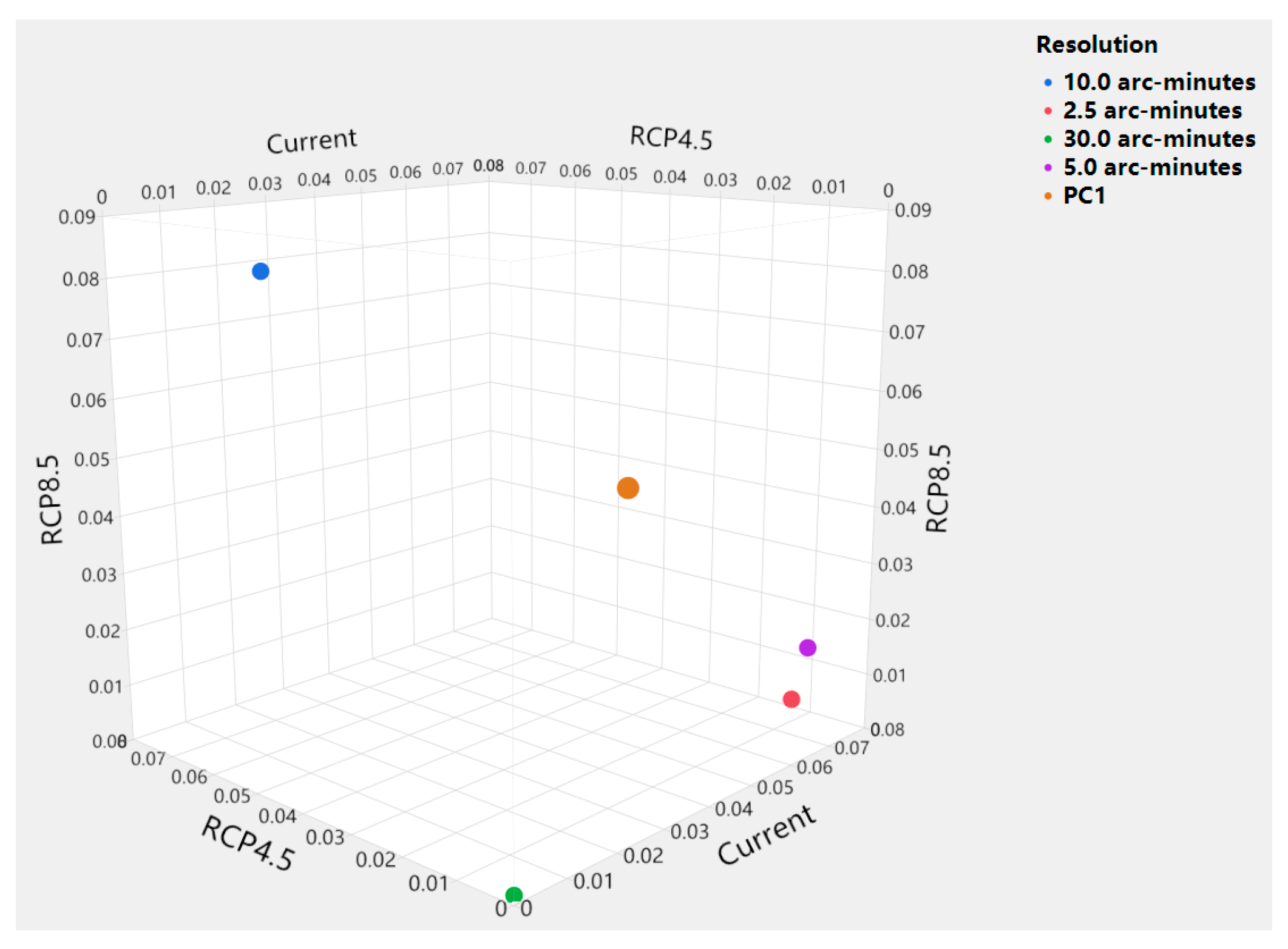
2.5. Scale-Balancing Method
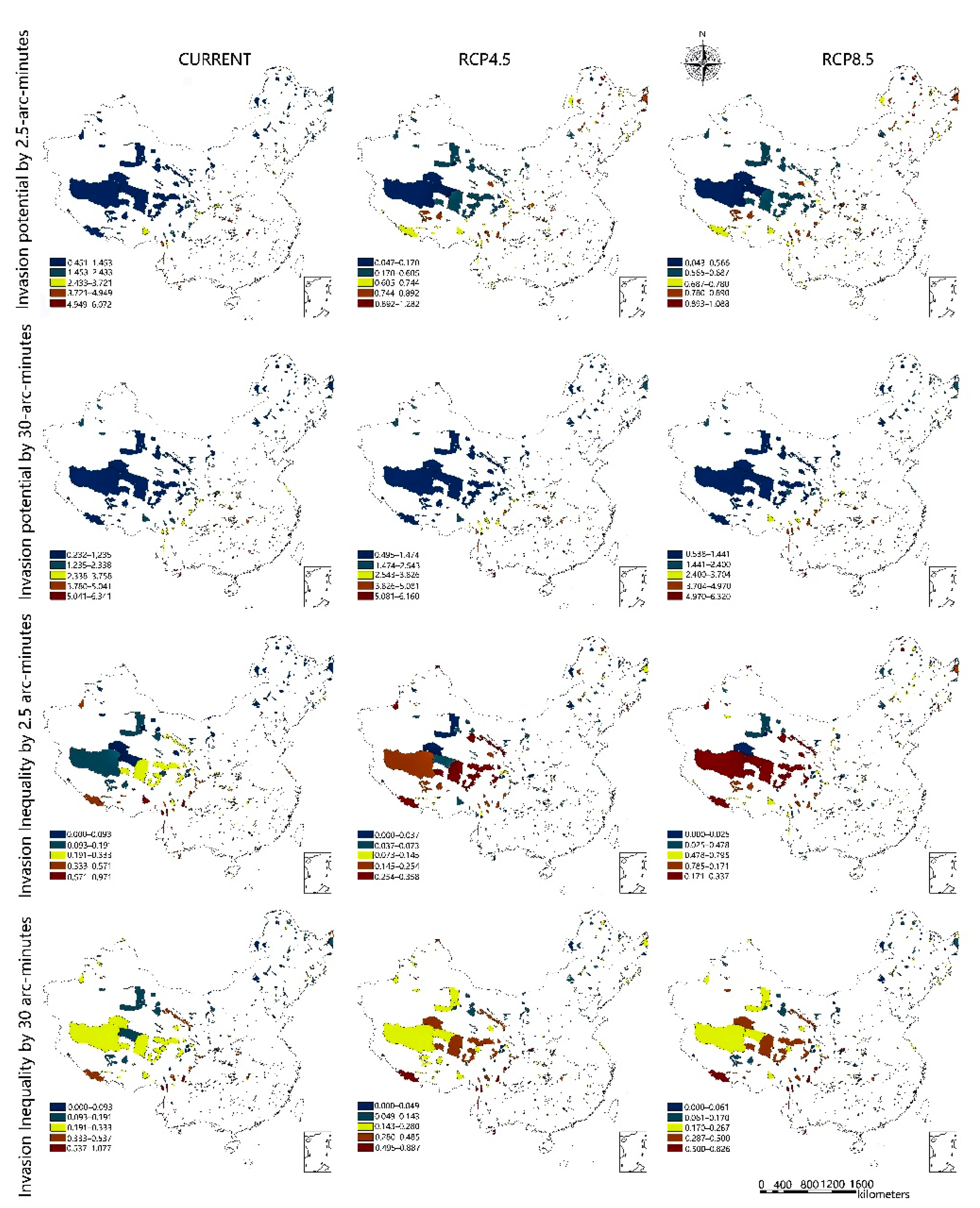
The use of different spatial scales can affect St and Dt as described above. Here, we need to determine an appropriate spatial scale to evaluate the risk and inequality of risk of IAPS for protected areas using PCA that uses St and Dt across different spatial scales. Some previous studies showed that the appropriate spatial scale was useful for SDMs such as Maxent [9,17,18]. Hence, we have aimed to propose a simple method to solve this specific problem. PCA is the most commonly used multivariate statistical analysis method to determine the principal components and select the appropriate variables accounting for the total variation (all scales [20,21]). PCA could explain most of the variation between different scales and help us select the most likely spatial scale based on relationships between two or more feature sets of source data (scale data: 2.5, 5.0, 10.0, and 30.0 arcminutes) in this study [9,17,19]. Hence, we combined the datasets of the risk of IAPS for protected areas across all scales into a single analysis.
First, we used St and Dt across different scales (2.5, 5.0, 10.0, and 30.0 arcminutes) as the PCA variables for the current concentration, low gas concentration, and high gas concentration, respectively. PCA was used to estimate the correlation matrix and percentage of variance of St and Dt, respectively. We used the St and Dt values of 2.5, 5.0, 10.0, and 30.0 arcminutes as the inputs of the PCA, respectively. We conducted PCA based on the correlation among these four resolutions (i.e., 2.5, 5.0, 10.0, and 30.0 arcminutes). We extracted the loadings of the first principal component (PC1) explaining more than 60% of the variance in St and Dt. The PC1 was significant (p < 0.001; Monte Carlo test) and accounted for more than a cumulative 60% of St and Dt across all spatial scales, respectively, for the current concentration, low gas concentration, and high gas concentration.
Second, we extracted the St and Dt scores of protected areas in the first principal component (PC1), respectively. PC1 was regarded as a single index representing the risk of IAPS for protected areas across all scales. Third, we separately assessed the relationship between IAPS risk and PC1 in protected areas at all scales (St and Dt) using simple linear regression analysis. This analysis was used to explore the bias of IAPS risk for protected areas between a certain scale and all scales. Fourth, we performed a simple linear regression analysis on the relationship between St and Dt (the results from all the scales and PC1). We aimed to explore the impact of scale effects on the relationship between St and Dt. Finally, we chose the appropriate spatial scales used for the risk of IAPS for protected areas under climate change based on two criteria: (1) the highest representativeness, accounting for the highest amounts of St and Dt at all scales (and the smallest bias of risk of IAPS for protected areas between a certain scale and all scales), and (2) the smallest impact of scale effects on the relationship between St and Dt.

3. Results

We found that an increase in the number of present records could reduce the accuracy of the SDMs (Figure 2). We found that there were significant relationships between fine scales and coarse scales in the current day and in the future (Table 1). The relationships between 2.5 arcminutes and the other three spatial scales were the largest for the potential of IAPS to invade protected areas and the inequality of IAPS invasion for protected areas (Table 1).
The most significant relationship was observed between the potential of IAPS to invade protected areas modeled with 5.0 arcminutes and PC1 in the present and future (St; average R2 = 95.92%; p < 0.001; Figure 3). The invasion inequality of IAPS for protected areas modeled with 5.0 arcminutes was also significantly related to PC1 in the present and future (Dt; average R2 = 89.23%; p < 0.001; Figure 3 and 2.5 arcminutes also showed a significant relationship with PC1 (average R2 = 92.75% for potential and R2 = 86.78% for inequality; p < 0.001; Figure 3). There was little bias in the invasion inequality of IAPS for protected areas between 2.5 arcminutes and 5.0 arcminutes. The scale of 5.0 arcminutes was the most consistent when using PC1 of these two indicators to evaluate the risk of IAPS for protected areas (Figure 4). However, above all, we used 5.0 arcminutes to evaluate the risk of IAPS for protected areas via the potential of IAPS to invade protected areas (St; Figure 4). Based on 2.5 arcminutes and 30 arcminutes, most protected areas that were invaded by IAPS were distributed in southern China under climate change (Figure 5; Table S2). The protected areas, including Damingshan, Dayaoshan, Yunkaishan, Maolan, Qianjiadong, and Yongzhoudoupangling, were shown to be significantly invaded by IAPS in the present and the future (Figure 5; Table S2).

4. Discussion

We built on a simple method that uses PCA to amalgamate different scales into SDMs when predicting the potential distributions of species and used our method to evaluate the risk of IAPS for protected areas in mainland China. We were able to use the linear relationship between the results of SDMs from different scales to select an appropriate scale to model the potential distributions of species. The results showed that the AUC values were significant, which ensures the accuracy and credibility of the experimental results. Here, increasing records may weaken the performance of SDMs, which may be affected by the uncertainties in the GBIF and CVH data. The increase in records could be enriching the distribution in areas where it had not been recorded, and with other environmental conditions that also enrich the bioclimatic profiles of the species. Coarse scales can lead to a small number of occurrence records. Hence, it is possible that coarse scales can lead to high accuracy in SDM for predicting IAPS distributions under climate change.
Wang et al. [16] found that the patterns and determinants of species richness vary on different spatial scales. The reasons for this might include (1) the scale effect of large-scale ecology, with the effect of climate change increasing relative to species richness with decreasing scales of resolution [31], and (2) cases in which the power of the climate, including environmental energy, water resource availability, and climate seasonality, increase with geographic expansion while the power of habitat heterogeneity and human activity declines [16]. At small scales, the dispersal of IAPS and human disturbance (e.g., changes in land use) made large contributions to the development of suitable habitats for IAPS. IAPS distributions were more strongly influenced by dispersal limitations. Human disturbance can change global land cover, resulting in ecosystem fragmentation, habitat loss, and consequent changes in the local distributions of IAPS. Hence, we should identify the forms of dispersal of IAPS, and incorporate changes in land use into SDMs [16,31,32]. Hence, modeling the potential distributions of multiple species was influenced by the spatial scale. We need to determine the scale units to model the potential distributions of species with a fine or increasingly coarse resolution. Franklin et al. [17] studied the impact of using various scales on plant species distributions and proposed that it is necessary to balance fine and coarse scales. Some studies have found that there was a bias in the scale effect for the results of SDMs when using fine scales or coarse scales, and this indicated that the selection of scales may lead to an over- or underestimation of the potential distributions of species [18,19]. We also found that the extent of the differences in the results of Maxent—namely, the invasion risk—for different scales suggested this pattern in our study.
The effect of scale can be solved by applying a scale balance to the SDM results of Maxent based on the relationship between the potential distributions of species on fine scales or coarse scales [12,30,31]. Here, we used PC1 as the indicator representing all scales, and PC1 could explain most of the SDM results across all scales. We selected the most appropriate scale related to PC1. Our main objective was to select the scale that could reduce the difference between SDM results across all scales due to the scale effect. Thus, we could select the appropriate scale based on the relationship between the scales and PC1. We used the case of the invasion of IAPS into Chinese protected areas to explore the effect of applying a scale balance to the SDM results of Maxent using fine and increasingly coarse scales.
Previous studies [17,18,33,34] showed the impact of the scale effect on the results of SDMs (e.g., Maxent) and indicated that the fine scales were fit for modeling the potential distributions of species. However, several studies have also used coarse scales to map the distributions of species [4,15,35,36]. Hence, our suggestion was to use different scales of resolution as the inputs of SDMs, and then a simple method to integrate various scales into SDMs was proposed. We found that 2.5 arcminutes and 5.0 arcminutes were the most appropriate for the evaluation of the risk of IAPS for protected areas (2.5 arcminutes and 5.0 arcminutes for the invasion inequality of IAPS for protected areas and 5.0 arcminutes for the potential of IAPS to invade protected areas). Hence, 5.0 arcminutes could account for most scales and demonstrated the weakest effect of scale on the potential distributions of multiple species. We also found an interesting result in that there was a significant relationship between the potential of IAPS to invade protected areas and the invasion inequality of IAPS for protected areas across all scales, and 5.0 arcminutes was the most consistent with PC1 for these two indicators. To summarize, we used 5.0 arcminutes to evaluate the risk of IAPS in protected areas.
Some researchers have used SDMs to model the potential distributions of species in protected areas, including endangered species and IAPS [4,37,38,39,40]. Here, we predicted the potential distributions of IAPS in Chinese protected areas and found that Damingshan, Dayaoshan, Yunkaishan, Maolan, Qianjiadong, and Yongzhoudoupangling would be significantly invaded by IAPS, which indicates that we need to conduct long-term monitoring of these protected areas, particularly grids with a high possibility for the invasion of IAPS, to prevent the invasive spread of IAPS because of climate change [41,42]. More importantly, our finding that there was a significant relationship in terms of invasion risk between the present day and the future suggests that we should attach importance to the current risk of IAPS for protected areas.
How can we evaluate the risk of IAPS for protected areas under climate change? We used the ability of IAPS to invade protected areas to assess the risk of IAPS for the overall protected area and the invasion inequality of IAPS for protected areas for part of the protected area. A study by Araújo et al. (2011), who used SDMs to assess the ability of protected areas to protect endangered species under climate change, provided insights into evaluating the risk of IAPS for protected areas [4,43]. We regarded a large proportion of suitable habitats of IAPS as having a high risk in the overall protected area. The current level of protected areas invaded by IAPS was consistent with the future when following the patterns of greenhouse gas emissions. However, we also found that greenhouse gas emissions, particularly in the high-emissions scenario, will increase the uncertainty of the change in IAPS risks for protected areas. We should not ignore the differentiation of IAPS invasions into different parts of protected areas. For the protected areas violently invaded by IAPS, the high invasion inequality of IAPS indicated that the difference in habitat quality was large, and vice versa. Hence, the invasion inequality reflected the risk areas of IAPS at some levels. For protected areas with high invasion inequality, we should take conservation actions based on the parts of protected areas while attaching importance to the protected areas invaded by IAPS. If the protected areas have low invasion inequality in terms of IAPS, the regions with high habitat quality are a key consideration for protected areas with high IAPS invasion risks [44]. Greenhouse gas emissions could enhance the relationship between the invasion ability and invasion inequality of IAPS for protected areas [45]. This indicates that future invasions of IAPS will be more intensely focused on protected areas compared to those of the present day. Our findings suggested that we need to strengthen ecological monitoring to find highly suitable habitats for IAPS in protected areas. Hence, our method could provide conservation suggestions for the assessment scales of invasive species used by biological conservationists and land managers. Can we evaluate the risk of IAPS on finer scales, such as the grid of protected areas? We need to solve the problem of how spatial scales affect habitat quality.
Modeling the habitat quality of species was influenced by the spatial scale of climate change. We aimed to determine the scale units to model the habitat quality of species—a fine resolution or coarse resolution [46]. This led us to question of whether SDM results obtained using different scales were accurate. The results obtained from Maxent for all scales were positively related to the regions’ species richness, indicating that the habitat quality of species at different scales was useful for long-term management [18]. Franklin et al. (2013) studied the impact of the use of various scales on plant species’ distributions and proposed that it is necessary to balance fine and coarse scales [17]. Some studies have found that there is an important relationship between habitat quality when using fine scales or coarse scales, and this indicates that scale selection might overestimate or underestimate SDM outcomes [12,17,18,46]. We also found that the extent of the difference in the results of Maxent—namely, the invasion risk—of different scales suggested this pattern in our study. This problem can be solved by applying a scale balance to the SDM results of Maxent based on the relationship between habitat quality using fine scales or coarse scales [17,47].
PCA is the most commonly used multivariate statistical analysis tool to select the appropriate variables accounting for the total variation [20,21]. Hence, we could balance the biases of IAPS risk that occurred when fine or coarse scales were used in the estimates. Recent studies have shown that fine scales can reduce uncertainty when modeling regional habitat quality [9,17,18]. The finding that the invasion inequality of IAPS for protected areas at the finest scales could account for all scales was consistent with the findings of previous studies [17]. It is necessary to conduct long-term monitoring of protected areas, particularly grids with highly suitable habitats for IAPS to prevent the invasive spread of IAPS that is due to climate change [46]. However, we used 5.0 arcminutes to predict the ability of IAPS to invade protected areas because 5.0 arcminutes had a significant relationship with each spatial scale and represented the results of all scales [48,49].
We invented a simple and convenient method to balance the various results of modeling at different spatial scales to prevent the overestimation or underestimation of SDM results caused by the selection of the spatial scale and to consider the impact of different scales on SDM results. In China, between the west and the east there is a substantial difference of almost 3000 km, as well as a latitudinal gradient of around 2000 km, making it difficult to use the same eight variables for all species. Perhaps this is possible when using a coarse spatial resolution, but it minimizes environmental variation in large areas of the country according to the resolution used. Hence, 5.0 arcminutes were relatively coarse for SDM applications in predictions of the distributions of IAPS compared to previous studies.
We should emphasize that conservation measures cannot afford to wait until there is enough information available on IAPS [46]. Our study provides a great example of the use of SDMs: for instance, the application of Maxent to biological conservation and ecological risk assessment. Here, we offer helpful suggestions to assess the risk of invasive species: (1) it is necessary to calculate two metrics, the ability of IAPS to invade protected areas and the invasion inequality of IAPS in protected areas; (2) the various effects of different spatial scales on the results of SDMs should be balanced; and (3) we should determine the regional scales of IAPS risk for the overall part or grid of a region. The effect of scale on the outcomes of SDMs still perplexes researchers and land managers and makes it impossible for them to use data to make reasonable and accurate decisions regarding biological conservation policies [9,17,19]. Therefore, we have attempted to put forward a method to balance the results of SDMs across all scales and used the fitted results to determine the risk of IAPS for regions [50,51,52,53]. Despite the limited number of studies conducted on ecological validation methods such as ecological monitoring and field investigation, there is an urgent need for innovative assessment approaches and tools to predict invasive species distributions and assess the invasive risks of species at different spatial scales [54,55,56].

5. Conclusions

We must emphasize that conservation measures cannot afford to wait until there is enough information available on IAPS. This study provides a good example of the application of SDMs to biological conservation and ecological risk assessment. First, we attached importance to the selection of the resolution (2.5, 5.0, 10.0, and 30.0 arcminutes) because these four resolutions have been widely used in studies using SDMs around the world. Hence, we used the method of our study to select the appropriate scale as the input of SDMs. Second, we computed two indicators: the potential of IAPS to invade protected areas and the invasion inequality of IAPS in protected areas. Third, the various impacts of different spatial scales on the results of SDMs should be balanced. The effect of scale on the results of SDMs still perplexes researchers and land managers and keeps them from using data to make reasonable and accurate decisions regarding biological conservation policies. Finally, we hope that future research will expand on the application of SDMs to provide actionable recommendations for the risk evaluation of invasive species under climate change.

Supplementary Materials

The following supporting information can be downloaded at https://www.mdpi.com/article/10.3390/app122111108/s1: Table S1: Occurrence records of IAPS; Table S2: The potential of IAPS to invade protected areas and the invasion inequality of IAPS for protected areas.

Author Contributions

Conceptualization, J.-Z.W. and C.-J.W.; methodology, J.-Z.W.; software, J.-Z.W.; validation, D.-J.X., J.-Z.W. and C.-J.W.; formal analysis, F.-X.Z.; investigation, J.-Z.W.; resources, J.-Z.W.; data curation, J.-Z.W. and C.-J.W.; writing—original draft preparation, D.-J.X., J.-Z.W. and C.-J.W.; writing—review and editing, D.-J.X., J.-Z.W. and C.-J.W.; visualization, J.-Z.W.; supervision, D.-J.X.; project administration, D.-J.X. and C.-J.W.; funding acquisition, D.-J.X. All authors have read and agreed to the published version of the manuscript.

Funding

This work has been supported by the Scientific and Technological Achievements Transformation Project of Qinghai Science and Technology Department (No. 2021-SF-152), the Youth Project Research Foundation of Qinghai University, China (No. 2019-QNY-1), and the First Subsidy Funds for Forestry Development and Reform in 2022 (No. 2022-358): Wetland Conservation and Restoration Project for Beichuan River Source Region National Nature Reserve in Datong County, Qinghai Province, China.

Institutional Review Board Statement

Not applicable.

Informed Consent Statement

Not applicable.

Data Availability Statement

Not applicable.

Acknowledgments

We thank Feng Xiao from Wetland Conservation Center of Qinghai Province and Fei-Hai Yu and CVH for the comments on occurrence records.

Conflicts of Interest

The authors declare no conflict to interest.

References

  1. Elith, J.; Phillips, S.J.; Hastie, T.; Dudík, M.; Chee, Y.E.; Yates, C.J. A statistical explanation of MaxEnt for ecologists. Divers. Distrib. 2011, 17, 43–57. [Google Scholar] [CrossRef]
  2. Dubey, S.; Pike, D.A.; Shine, R. Predicting the impacts of climate change on genetic diversity in an endangered lizard species. Clim. Chang. 2014, 117, 319–327. [Google Scholar] [CrossRef] [Green Version]
  3. Wang, A.; Melton, A.E.; Soltis, D.E.; Soltis, P.S. Potential distributional shifts in North America of allelopathic invasive plant species under climate change models. Plant Divers. 2022, 44, 11–19. [Google Scholar] [CrossRef] [PubMed]
  4. Araújo, M.B.; Alagador, D.; Cabeza, M.; Nogués-Bravo, D.; Thuiller, W. Climate change threatens European conservation areas. Ecol. Lett. 2011, 14, 484–492. [Google Scholar] [CrossRef] [PubMed] [Green Version]
  5. Bellard, C.; Thuiller, W.; Leroy, B.; Genovesi, P.; Bakkenes, M.; Courchamp, F. Will climate change promote future invasions? Glob. Chang. Biol. 2013, 19, 3740–3748. [Google Scholar] [CrossRef] [PubMed]
  6. Wang, C.J.; Wang, R.; Yu, C.M.; Dang, X.P.; Sun, W.G.; Li, Q.F.; Wang, X.T.; Wan, J.Z. Risk assessment of insect pest expansion in alpine ecosystems under climate change. Pest Manag. Sci. 2021, 77, 3165–3178. [Google Scholar] [CrossRef]
  7. Zhang, F.X.; Wang, C.J.; Wan, J.Z. Using Consensus Land Cover Data to Model Global Invasive Tree Species Distributions. Plants 2022, 11, 981. [Google Scholar] [CrossRef]
  8. Merow, C.; Smith, M.J.; Silander, J.A. A practical guide to MaxEnt for modeling species’ distributions: What it does, and why inputs and settings matter. Ecography 2013, 36, 1058–1069. [Google Scholar] [CrossRef]
  9. Borja, J.; David, D.; David, N. Modeling the potential area of occupancy at fine resolution may reduce uncertainty in species range estimates. Biol. Conserv. 2012, 147, 190–196. [Google Scholar]
  10. Pineda, E.; Lobo, J.M. The performance of range maps and species distribution models representing the geographic variation of species richness at different resolutions. Glob. Ecol. Biogeogr. 2012, 21, 935–944. [Google Scholar] [CrossRef]
  11. Lázaro-Lobo, A.; Ramirez-Reyes, C.; Lucardi, R.D.; Ervin, G.N. Multivariate analysis of invasive plant species distributions in southern US forests. Landsc. Ecol. 2021, 36, 3539–3555. [Google Scholar] [CrossRef]
  12. Wan, J.Z.; Wang, C.J.; Yu, F.H. Effects of occurrence record number, environmental variable number, and spatial scales on MaxEnt distribution modelling for invasive plants. Biologia 2019, 74, 757–766. [Google Scholar] [CrossRef]
  13. Connor, T.; Hull, V.; Viña, A.; Shortridge, A.; Tang, Y.; Zhang, J.; Liu, J. Effects of grain size and niche breadth on species distribution modeling. Ecography 2018, 41, 1270–1282. [Google Scholar] [CrossRef] [Green Version]
  14. Manzoor, S.A.; Griffiths, G.; Lukac, M. Species distribution model transferability and model grain size–finer may not always be better. Sci. Rep. 2018, 8, 7168. [Google Scholar] [CrossRef] [Green Version]
  15. Zhang, H.; Zhang, M. Insight into distribution patterns and conservation planning in relation to woody species diversity in Xinjiang, arid northwestern China. Biol. Conserv. 2014, 177, 165–173. [Google Scholar] [CrossRef]
  16. Wang, Z.; Rahbek, C.; Fang, J. Effects of geographical extent on the determinants of woody plant diversity. Ecography 2012, 35, 1160–1167. [Google Scholar] [CrossRef]
  17. Franklin, J.; Davis, F.W.; Ikegami, M.; Syphard, A.D.; Flint, L.E.; Flint, A.L.; Hannah, L. Modeling plant species distributions under future climates: How fine scale do climate projections need to be? Glob. Chang. Biol. 2013, 19, 473–483. [Google Scholar] [CrossRef] [Green Version]
  18. Bean, W.T.; Prugh, L.R.; Stafford, R.; Butterfield, H.S.; Westphal, M.; Brashares, J.S. Species distribution models of an endangered rodent offer conflicting measures of habitat quality at multiple scales. J. Appl. Ecol. 2014, 51, 1116–1125. [Google Scholar] [CrossRef]
  19. Suárez-Seoane, S.; Virgós, E.; Terroba, O.; Pardavila, X.; Barea-Azcón, J.M. Scaling of species distribution models across spatial resolutions and extents along a biogeographic gradient. The case of the Iberian mole Talpa occidentalis. Ecography 2014, 37, 279–292. [Google Scholar] [CrossRef]
  20. Metzger, M.J.; Bunce, R.G.H.; Jongman, R.H.G.; Mücher, C.A.; Watkins, J.W. A climatic stratification of the environment of Europe. Glob. Ecol. Biogeogr. 2005, 14, 549–563. [Google Scholar] [CrossRef]
  21. Tomas, J.B.; Amanda, E.B.; Jonathan, S.L.; Nicole, A.H.; Russell, J.T.; Graham, J.E.; Rick, D.S.; Simon, W.; Martin, K.; Jemina, F.S.; et al. Statistical solutions for error and bias in global citizen science datasets. Biol. Conserv. 2014, 173, 144–154. [Google Scholar]
  22. Gabriele, C.; Paolo, G.; Renato, B.; Bruno, F.; Daniele, V.; Rossella, F.; Emmanuele, F.; Simonetta, B.; Stefania, P.; Mauro, G.M. Climate change hastens the urgency of conservation for range-restricted plant species in the central-northern Mediterranean region. Biol. Conserv. 2014, 179, 129–138. [Google Scholar]
  23. Gallien, L.; Münkemüller, T.; Albert, C.H.; Boulangeat, I.; Thuiller, W. Predicting potential distributions of invasive species: Where to go from here? Divers. Distrib. 2010, 16, 331–342. [Google Scholar] [CrossRef]
  24. Hernandez, P.A.; Graham, C.H.; Master, L.L.; Albert, D.L. The effect of sample size and species characteristics on performance of different species distribution modeling methods. Ecography 2006, 29, 773–785. [Google Scholar] [CrossRef]
  25. Hengl, T.; Mendes de Jesus, J.; Heuvelink, G.B.; Ruiperez Gonzalez, M.; Kilibarda, M.; Blagotić, A.; Kempen, B. SoilGrids250m: Global gridded soil information based on machine learning. PLoS ONE 2017, 12, e0169748. [Google Scholar] [CrossRef] [PubMed] [Green Version]
  26. Phillips, S.J.; Dudík, M. Modeling of species distributions with Maxent: New extensions and a comprehensive evaluation. Ecography 2008, 31, 161–175. [Google Scholar] [CrossRef]
  27. Hoffman, J.D.; Aguilar-Amuchastegui, N.; Tyre, A.J. Use of simulated data from a process-based habitat model to evaluate methods for predicting species occurrence. Ecography 2010, 33, 656–666. [Google Scholar] [CrossRef]
  28. Radosavljevic, A.; Anderson, R.P. Making better Maxent models of species distributions: Complexity, overfitting and evaluation. J. Biogeogr. 2014, 41, 629–643. [Google Scholar] [CrossRef]
  29. Kuebbing, S.E.; Nuñez, M.A.; Simberloff, D. Current mismatch between research and conservation efforts: The need to study co-occurring invasive plant species. Biol. Conserv. 2013, 160, 121–129. [Google Scholar] [CrossRef]
  30. Calabrese, J.M.; Certain, G.; Kraan, C.; Dormann, C.F. Stacking species distribution models and adjusting bias by linking them to macroecological models. Glob. Ecol. Biogeogr. 2014, 23, 99–112. [Google Scholar] [CrossRef]
  31. Rahbek, C.; Graves, G.R. Multiscale assessment of patterns of avian species richness. Proc. Natl. Acad. Sci. USA 2001, 98, 4534–4539. [Google Scholar] [CrossRef] [PubMed] [Green Version]
  32. Václavík, T.; Kupfer, J.A.; Meentemeyer, R.K. Accounting for multi-scale spatial autocorrelation improves performance of invasive species distribution modelling (iSDM). J. Biogeogr. 2012, 39, 42–55. [Google Scholar] [CrossRef]
  33. Alsamadisi, A.G.; Tran, L.T.; Papeş, M. Employing inferences across scales: Integrating spatial data with different resolutions to enhance Maxent models. Ecol. Model. 2020, 415, 108857. [Google Scholar] [CrossRef]
  34. Schmidt, H.; Radinger, J.; Teschlade, D.; Stoll, S. The role of spatial units in modelling freshwater fish distributions: Comparing a subcatchment and river network approach using MaxEnt. Ecol. Model. 2020, 418, 108937. [Google Scholar] [CrossRef]
  35. Zhang, M.G.; Zhou, Z.K.; Chen, W.Y.; Cannon, C.H.; Raes, N.; Slik, J.W. Major declines of woody plant species ranges under climate change in Yunnan, China. Divers. Distrib. 2014, 20, 405–415. [Google Scholar] [CrossRef]
  36. Gallagher, R.V.; Hughes, L.; Leishman, M.R. Species loss and gain in communities under future climate change: Consequences for functional diversity. Ecography 2013, 36, 531–540. [Google Scholar] [CrossRef]
  37. Velásquez-Tibatá, J.; Salaman, P.; Graham, C.H. Effects of climate change on species distribution, community structure, and conservation of birds in protected areas in Colombia. Reg. Environ. Chang. 2013, 13, 235–248. [Google Scholar] [CrossRef]
  38. Vicente, J.R.; Fernandes, R.F.; Randin, C.F.; Broennimann, O.; Gonçalves, J.; Marcos, B.; Pôcas, I.; Alves, P.; Guisan, A.; Honrado, J.P. Will climate change drive alien invasive plants into areas of high protection value? An improved model-based regional assessment to prioritise the management of invasions. J. Environ. Manag. 2013, 131, 185–195. [Google Scholar] [CrossRef]
  39. Cotrina Sánchez, A.; Rojas Briceño, N.B.; Bandopadhyay, S.; Ghosh, S.; Torres Guzmán, C.; Oliva, M.; Salas López, R. Biogeographic Distribution of Cedrela spp. Genus in Peru Using MaxEnt Modeling: A Conservation and Restoration Approach. Diversity 2021, 13, 261. [Google Scholar] [CrossRef]
  40. Chen, K.; Wang, B.; Chen, C.; Zhou, G. MaxEnt Modeling to Predict the Current and Future Distribution of Pomatosace filicula under Climate Change Scenarios on the Qinghai–Tibet Plateau. Plants 2022, 11, 670. [Google Scholar] [CrossRef]
  41. Caplat, P.; Cheptou, P.O.; Diez, J.; Guisan, A.; Larson, B.M.H.; Macdougall, A.S.; Peltzer, D.A.; Richardson, D.M.; Shea, K.; van Kleunen, M.; et al. Movement, impacts and management of plant distributions in response to climate change: Insights from invasions. Oikos 2013, 122, 1265–1274. [Google Scholar] [CrossRef] [Green Version]
  42. O’Neill, M.W.; Bradley, B.A.; Allen, J.M. Hotspots of invasive plant abundance are geographically distinct from hotspots of establishment. Biol. Invasions 2021, 23, 1249–1261. [Google Scholar] [CrossRef]
  43. Yu, J.; Wang, C.; Wan, J.; Han, S.; Wang, Q.; Nie, S. A model-based method to evaluate the ability of nature reserves to protect endangered tree species in the context of climate change. For. Ecol. Manag. 2014, 327, 48–54. [Google Scholar] [CrossRef]
  44. Wang, C.J.; Wan, J.Z.; Zhang, G.M.; Zhang, Z.X.; Zhang, J. Protected areas may not effectively support conservation of endangered forest plants under climate change. Environ. Earth Sci. 2016, 75, 46. [Google Scholar]
  45. Zhang, L.; Wang, S.L.; Liu, S.W.; Liu, X.J.; Zou, J.W.; Sieman, E. Perennial forb invasions alter greenhouse gas balance between ecosystem and atmosphere in an annual grassland in China. Sci. Total Environ. 2018, 642, 781–788. [Google Scholar] [CrossRef]
  46. Wan, J.Z.; Wang, C.J.; Yu, F.H. Impacts of the spatial scale of climate data on the modeled distribution probabilities of invasive tree species throughout the world. Ecol. Inform. 2016, 36, 42–49. [Google Scholar] [CrossRef]
  47. Guisan, A.; Graham, C.H.; Elith, J.; Huettmann, F. Sensitivity of predictive species distribution models to change in grain size. Divers. Distrib. 2007, 13, 332–340. [Google Scholar] [CrossRef]
  48. Kramer-Schadt, S.; Niedballa, J.; Pilgrim, J.D.; Schröder, B.; Lindenborn, J.; Reinfelder, V.; Stillfried, M.; Heckmann, I.; Scharf, A.K.; Augeri, D.M. The importance of correcting for sampling bias in MaxEnt species distribution models. Divers. Distrib. 2013, 19, 1366–1379. [Google Scholar] [CrossRef]
  49. Gueta, T.; Carmel, Y. Quantifying the value of user-level data cleaning for big data: A case study using mammal distribution models. Ecol. Inform. 2016, 34, 139–145. [Google Scholar] [CrossRef]
  50. Thuiller, W.; Richardson, D.M.; Pyšek, P.; Midgley, G.F.; Hughes, G.O.; Rouget, M. Niche-based modelling as a tool for predicting the risk of alien plant invasions at a global scale. Glob. Chang. Biol. 2005, 11, 2234–2250. [Google Scholar] [CrossRef]
  51. Donaldson, J.E.; Hui, C.; Richardson, D.M.; Robertson, M.P.; NWebber, B.L.; Wilson, J.R. Invasion trajectory of alien trees: The role of introduction pathway and planting history. Glob. Chang. Biol. 2014, 20, 1527–1537. [Google Scholar] [CrossRef] [PubMed]
  52. Mainali, K.P.; Warren, D.L.; Dhileepan, K.; McConnachie, A.; Strathie, L.; Hassan, G.; Karki, D.; Shrestha, B.B.; Parmesan, C. Projecting future expansion of invasive species: Comparing and improving methodologies for species distribution modeling. Glob. Chang. Biol. 2015, 21, 4464–4480. [Google Scholar] [CrossRef] [PubMed] [Green Version]
  53. Richardson, D.M. Conservation biogeography: What’s hot and what’s not? Divers. Distrib. 2012, 18, 319–322. [Google Scholar] [CrossRef]
  54. Miller, A.J.; Knouft, J.H. GIS-based characterization of the geographic distributions of wild and cultivated populations of the Mesoamerican fruit tree Spondias purpurea (Anacardiaceae). Am. J. Bot. 2006, 93, 1757–1767. [Google Scholar] [CrossRef] [PubMed]
  55. Wang, C.J.; Wan, J.Z.; Zhang, Z.X. Expansion potential of invasive tree plants in ecoregions under climate change scenarios: An assessment of 54 species at a global scale. Scand. J. For. Res. 2017, 32, 663–670. [Google Scholar] [CrossRef]
  56. Wan, J.Z.; Wang, C.J.; Yu, F.H. Risk hotspots for terrestrial plant invaders under climate change at the global scale. Environ. Earth Sci. 2016, 75, 1–8. [Google Scholar] [CrossRef]
Figure 1. The distribution map of the protected areas analyzed in this study.
Applsci 12 11108 g001
Figure 2. The records and AUC values for nine IAPS.
Applsci 12 11108 g002
Figure 3. The linear relationship (coefficient of determination; R2) of risk of IAPS for protected areas, comparing different scales of resolution (i.e., 0.5 arcminutes, 2.5 arcminutes, 5.0 arcminutes, and 10.0 arcminutes) and PC1 in different concentration scenarios. Current: the present day; RCP4.5: low-gas-concentration scenario; RCP8.5: high-gas-concentration scenario; 0.5: 0.5 arcminutes; 2.5: 2.5 arcminutes; 5.0: 5.0 arcminutes; 10.0: 10.0 arcminutes. All the relationships were significant (i.e., p < 0.001).
Applsci 12 11108 g003
Figure 4. The linear relationships (coefficient of determination; R2) between the invasion potential of IAPS and the invasion inequality of IAPS for protected areas across all the scales and PC1. Current: the present day; RCP4.5: low-gas-concentration scenario; RCP8.5: high-gas-concentration scenario.
Applsci 12 11108 g004
Figure 5. The potential of IAPS-invaded protected areas and the inequality of IAPS-invaded protected areas at both 2.5 arcminutes and 30.0 arcminutes under climate change. Current: the present day; RCP4.5: low-gas-concentration scenario; RCP8.5: high-gas-concentration scenario.
Applsci 12 11108 g005
Table 1. The relationships between the potential presence of IAPS-invaded protected areas and the inequality of IAPS-invaded protected areas; 0.5: 0.5 arcminutes; 2.5: 2.5 arcminutes; 5.0: 5.0 arcminutes; 10.0: 10.0 arcminutes. All the relationships were significant (p < 0.001).
PotentialInequality
2.5510302.551030
2.510.99870.99350.943810.9490.77110.4126
50.998710.99520.94730.94910.78820.4057
100.99350.995210.95360.77110.788210.4616
300.94380.94730.953610.41260.40570.46161
Publisher’s Note: MDPI stays neutral with regard to jurisdictional claims in published maps and institutional affiliations.

