Two-Stage Metaheuristic Algorithms for Order-Batching and Routing Problems

Abstract

Because of time and cost constraints, item picking plays a major role in warehouse operations. Considering diversified orders and a constant warehouse design, deciding how to combine each batch and picker route effectively is a challenge in warehouse management. In this study, we focus on the evaluation of order-batching strategies for a single picker facing multiple orders with the objective of minimizing the total traveling distance. We propose two-stage simulated annealing and variable neighborhood search algorithms to solve the combined problem. The orders are first merged into batches, followed by determining the sequence in each batch. The computational analysis revealed that the best-fit-decreasing (BFD) batch ordering strategy in the two-stage algorithms, the variable neighborhood search algorithm, obtained superior solutions to those of the simulated annealing algorithm.

1. Introduction

Achieving high efficiency in order batching and picking operations has become highly crucial. To achieve low-cost and large-quantity throughput with fast delivery, batching and picking operations are the most effective picking activities. Picking time constitutes approximately 30–40% of the total working hours, and labor cost constitutes 15–20% of the total cost; moreover, traveling and picking time form 60% and 20%, respectively, of the total picking time [1]. Consequently, effectively reducing operating costs necessitates focusing on enhancing the efficiency of traveling and picking procedures.

Warehouse management involves several categories, including storage planning, order batching, order picking, warehouse layout design, and storage policies [2]. The major challenge in warehouse management is the planning required to reduce the time, cost, and distance in picking operations. Regarding batching and picking problems, the major objective of this study is to effectively obtain an optimal solution within a limited time frame. We adopted the model of batching and picking problems proposed by Kulak et al. [3] as the study background and proposed five batch ordering strategies with two-stage simulated annealing (SA) and variable neighborhood search (VNS) algorithms to improve the solution. Finally, the results were compared with the same questions to determine which batch ordering strategy can quickly and effectively obtain solutions.

The rest of this paper is organized as follows. Section 2 describes related work, and Section 3 introduces the integrated order-batching and routing problem, and presents the formulation of a mixed-integer optimization model. The two-stage SA and VNS algorithms proposed for deriving near-optimal solutions are presented in Section 4. Section 5 presents the performance evaluation of the proposed algorithms, conducted through computational analysis. The final section provides the conclusion and potential applications of the proposed algorithms.

2. Literature Review

In the literature, most studies on warehouse order picking have focused only on picker routing or order batching. Articles that only consider order picking can be classified into certain [4,5,6,7,8,9,10,11,12,13,14,15,16,17] and uncertain cases [18,19]. Picker routing can be considered a traditional traveling-salesman problem (TSP). Through the distance between storage spaces, pickers plan how to visit each storage space through the shortest path before returning to the starting point. However, when the number of storage spaces increases, the computation time required to obtain an optimal solution is long [20]. Among the certain cases, many studies have considered the operating environment of AS/RS [4,5,10,11,12,13,14,17]. Storage systems, capacity, and strategies were introduced in [14,17]. Zone picking was used as the picking method in [8,15,16]. Petersen [21] evaluated the returning characteristic in routing policies to ensure that pickers enter an aisle to collect the required items, exit through the path they entered, and then, travel to subsequent aisles in succession. Regarding algorithm design, the genetic algorithm (GA) can be seen in [9,15].

In the area of order batching, most of the papers are certain cases [22,23,24,25,26,27,28,29,30,31,32,33,34]. Uncertain issues can only be seen in [35,36]. Hwang and Kim [25] developed an order-batching algorithm that is based on cluster analysis by considering three outing policies, namely traversal, return, and midpoint routing. Moreover, De Koster et al. [37] applied the midpoint method in which pickers enter from one end of an aisle to pick goods, and then, turn to another aisle in succession as each aisle is completed. Henn and Wäscher [38] resolved the question of how to combine customer orders to shorten the total picking distance. They suggested two metaheuristic algorithms, namely a classic tabu search (TS) algorithm and an attribute-based hill-climbing approach, and both approaches were superior to existing methods. Hwang et al. [39] solved batch order processing as a clustering problem. They defined items as attribute vectors and used three similarity measures to develop six cluster classification algorithms. The experimental results proved that merging orders with higher degrees of similarity improved the picking efficiency. The heterogeneous pick devices [34] and multiple pickers [36] were extended to the batching problem. Regarding the algorithm design, GA [28,31,33] and VNS [29,34,36] were widely introduced.

Among the integration issues considered together with order picking and order batching, we can see that most of them are certain issues [3,40,41,42,43,44,45,46,47,48,49,50] and uncertain issues can be found in [51,52]. The concept of storage systems, capacity, and strategy was introduced in [45,51]. Yu and Koster [52] used AS/RS as the operating environment.

Regarding the algorithm design, Won and Olafasson [40] solved the order-batching and picking-sequence problem by using hybrid heuristic algorithms. The first heuristic determines order batching, and the second heuristic identifies the picking sequence. Kulak et al. al. [3] and Henn [44] used TS to deal with the problem of order batching, while on the issue of picking, Kulak et al. [3] adopted a 2-opt method, and Henn [44] proposed a picking strategy. Tsai et al. [53] employed a two-stage GA to solve an order-batching and picking-sequence problem. The objective was to minimize the total traveling time. The first stage of the GA involved determining the order batches, and the second stage entailed determining the shortest picking paths for these batches. Lin et al. [48] considered a picking route based on the Manhattan distance and used particle swarm optimization (PSO) to solve the joint order-batching and picking-route problem. Cheng et al. [47] used PSO to deal with order batching and used ACO to find the most efficient route for each batch. Van Gils [49] set high customer service level and improved picking efficiency as its goals and developed an iterated local search algorithm to solve.

3. Problem Statement

This study deals with the order-batching problem and picking-route-sequence problem in the picker-to-part system; that is, in the conventional rectangular warehouse, the different orders are first classified and sorted into batches, with group orders with similar paths grouped together as much as possible. For the items to be picked in order, $O_k$, $i$, $B{O}_l$, and $D_{O_k/B{O}_l}$ represent the $k$-th order, storage location $i$, $l$-th batch, and the picking distance of order k or batch $l$, respectively. m represents the distance unit. $O_1$ = {$3, 6, 8$}, indicating that order 1 needs to be picked from storage positions 3, 6, and 8. If there are five orders, $O_1$ = {$3, 6, 8$}; $O_2$ =$\left\{62, 74, 80\right\}$; $O_3$ = {$2, 3, 4, 6, 7$}; $O_4$ = {$67, 74, 80$}; and $O_5$ = {$61, 62, 76, 80$} are to be classified into batches, and then, the distance of the orders individually calculated. 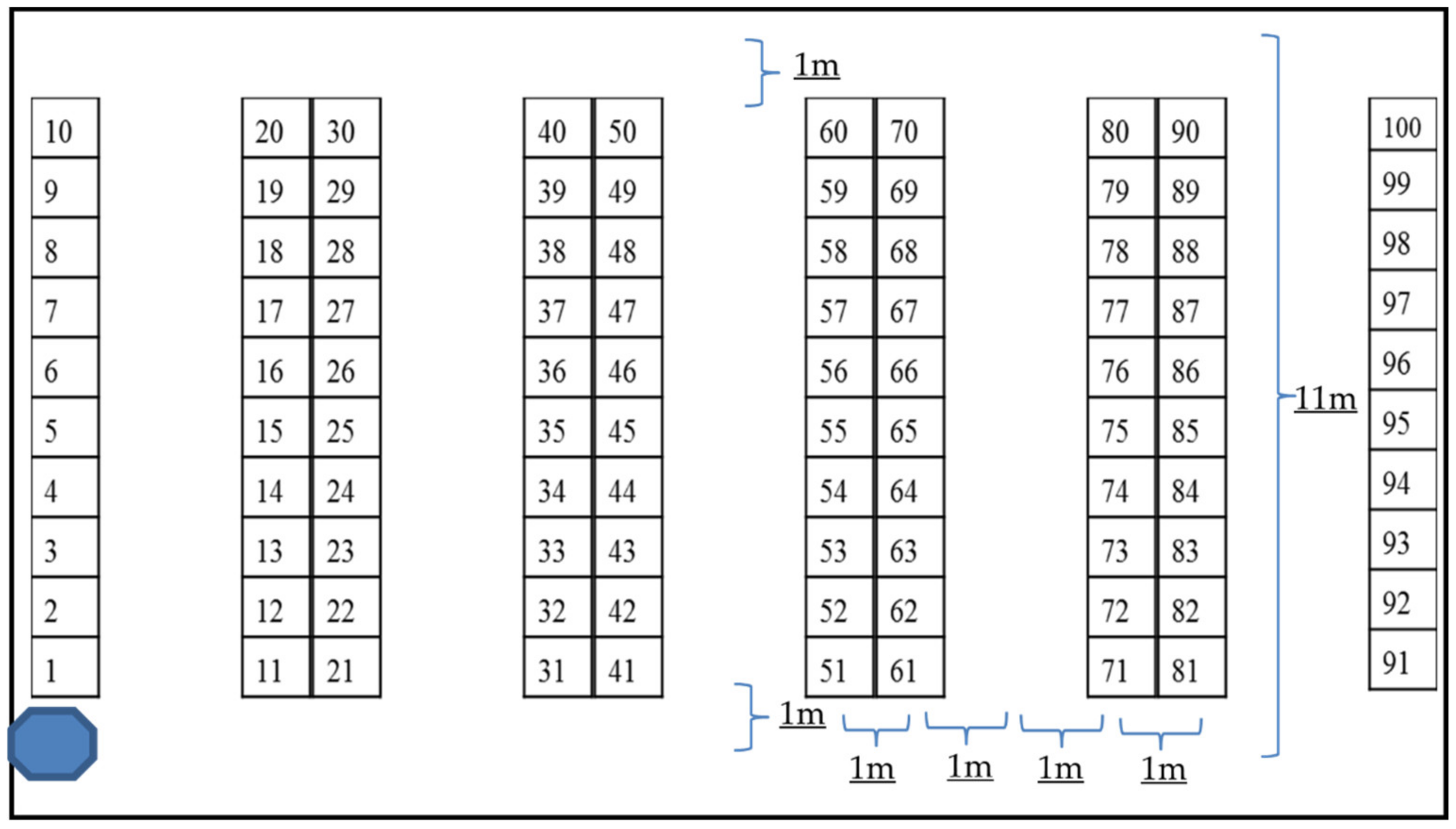As shown in Figure 1 and Figure 2, if we pick the items by following the number sequence, in order 1, it takes 4 m to travel from the entrance to position 3, 3 m from position 3 to 6, 2 m from position 6 to 8, and 9 m from position 8 to the entrance and exit. Hence, the distances of order 1 to order 5, $D_{O_1}~D_{O_5}$, are 18 m, 40 m, 16 m, 46 m, and 40 m. Since order 1 and order 3 are both picked in the first aisle, they can be grouped into batch 1, $B{O}_1=\left\{2, 3, 4, 6, 7, 8\right\}$. The distance of batch 1,$D_{B{O}_1}$, is 18 m. Without order batching, the total distance of these two orders is 34 m. Orders 2, 4, and 5 can be classified into batch 2, $B{O}_j=\left\{61, 62,67,74, 76, 80\right\}$, based on a similar situation. If the items are picked by individual order, the total distance of these three orders is 126 m, but the distance of batch 2, $D_{B{O}_2}$, is largely decreased to 46 m.

After combining the orders into batches, the picker picks items in sequence according to the sorted picking list of the batch, but if the picking route is different, the picker might go as far as possible in the warehouse. For example, {37,64,21,19,43} and {19,37,21,43,64} are picking routes 1 and 2 of the order. The distances of picking routes 1 and 2 are 68 m and 42 m, respectively.

We adopted the model proposed by Kulak et al. [3] to address the batching and picking problems and minimize the overall route. The problem assumptions, notations, and model are as follows.

Problem Assumptions:

• Warehouses have a picker-to-part system and parallel aisles.
• The storage strategy is dedicated location, so each storage position has a fixed size. Only one item can be stored or picked, and the quantity of the same item being picked is fixed at one.
• There is only one picker; that is, there is only one picker on the aisle, and the picker will take the path with the shortest distance and will not choose the path that bypasses the aisle.
• It is prohibited to split the order into different batches, and the items in the order cannot be cut into different batches. The size of one order cannot be over the size of one batch.
• The picker can pass up and down the aisle and pick the item on the left or the right. The picker picks the item in front of the storage position, and the distance and time from the picker to the item can be ignored.
• The warehouse layout plan shown in Figure 2 is a conventional rectangular warehouse, starting from and finally returning to the I/O point to complete the closed loop. There are 10 storage spaces in a row—two rows on the left and right in one aisle, and five aisles, with a total of 100 storage positions.
• All customers are known in advance, and no orders will be inserted, reduced, or changed in the middle of the process.

Notations:

$b\in B:\mathrm{number} \mathrm{of} \mathrm{batches}$

$k\in K:\mathrm{number} \mathrm{of} \mathrm{orders}$

$i,j\in V:\mathrm{number} \mathrm{of} \mathrm{storages}$

$S\subset V:\mathrm{subset} \mathrm{of} \mathrm{storage}$

$C:\mathrm{picker} \mathrm{capacity}$

$w_k:\mathrm{weight} \mathrm{of} \mathrm{order} k$

$d_{ij}:\mathrm{distance} \mathrm{from} \mathrm{storage} i \mathrm{to} \mathrm{storage} j$

$s_{ik}=\left\{\begin{array}{c}1, \mathrm{item} \mathrm{in} \mathrm{the} \mathrm{order} k \mathrm{located} \mathrm{at} \mathrm{storage} \mathit{i} \\ 0, \mathrm{otherwise} \end{array}\right.$

$X_k^b=\left\{\begin{array}{c}1, \mathrm{order} \mathit{k} \mathrm{assigned} \mathrm{to} \mathrm{batch} \mathit{b} \\ 0, \mathrm{otherwise} \end{array}\right.$

$Y_{ij}^b=\left\{\begin{array}{c}1, \mathrm{batch} \mathit{b} \mathrm{traveled} \mathrm{from} \mathrm{storage} \mathit{j} \mathrm{to} \mathrm{storage} \mathit{i} \\ 0, \mathrm{otherwise} \end{array}\right.$

$Z_i^b=\left\{\begin{array}{c}1, \mathrm{batch} b \mathrm{visit} \mathrm{storage} i \\ 0, \mathrm{otherwise} \end{array}\right.$

$$\min Z={{\displaystyle \sum }}_{b\in B}{{\displaystyle \sum }}_{i\ne j\in V}{d}_{ij}{Y}_{ij}^b$$

(1)

Subject to:

$${{\displaystyle \sum }}_{j\in V,j\ne i}{Y}_{ij}^b=Z_i^b \forall b\in B, i\in V$$

(2)

$${{\displaystyle \sum }}_{i\in V,i\ne j}{Y}_{ij}^b=Z_j^b \forall b\in B, j\in V$$

(3)

$${{\displaystyle \sum }}_{i\in S,j\in V\backslash S}{Y}_{ij}^b\ge Z_i^b \forall b\in B, S\subset V$$

(4)

$$Z_i^b\ge s_{ik} ·X_k^b \forall b\in B, i\in V k\in K$$

(5)

$${{\displaystyle \sum }}_{b\in B}{X}_k^b=1 \forall k\in K$$

(6)

$${{\displaystyle \sum }}_{j\in V,j\ne i}{w}_k·X_k^b\le C \forall b\in B$$

(7)

$$X_k^b, Y_{ij}^b,Z_i^b\in 0,1 , \forall i,j\in V, b\in B,k\in K$$

(8)

Objective (1) represents the objective function of the total picker route distance of all batches. Constraints (2) and (3) indicate that in order to avoid repetitive calculations, storage i can serve as the depot and destination only once. In addition, the constraints can be used to express whether the batches in storage have been picked. Constraint (4) represents a subcycle-eliminating constraint that prevents the formation of subcycles. The limiting function ensures that all picking points are picked and that each storage unit that requires picking is picked only once. Constraint (5) forces the selected orders and items in a batch to transform into binary variables. Constraint (6) reveals that an order can be assigned to only one batch to prevent such an order from being repetitively assigned to various batches. Constraint (7) indicates the capacity of the picking vehicle, signifying that the batch weight after order consolidation cannot exceed the maximum vehicle load. Constraint (8) indicates that all variables are binary.

4. Proposed Algorithm

The concept of the proposed algorithm is to decompose the order-batching and picking-route problem into two independent algorithms. First, in the first algorithm (order batching), the encoding solution, obtained from the initial batch order or the order-batching neighborhood (mutation/swap), is the input of the second algorithm (picking route). In the second algorithm, the initial picking route is obtained from storage locations with lower numbers to those with high numbers. The picking-route neighborhood (swap/insert) is used to obtain the best route of the current batches. Then, the distance of the best route is the objective value (distance) of the first algorithm. The whole framework of the proposed algorithm can be seen in Figure 3.

4.1. Initial Batch Order

Through order consolidation, each reduced batch can shorten the picking route of an order. Consequently, the only factor considered in determining the initial batch is capacity restriction. Moreover, we excluded route proximity from the criteria used to determine the initial batch. We considered five approaches for obtaining the initial solutions of the batching problem, and among these approaches, the picking route was not considered. The single-order (SO) method differs from the other methods, and this method involves considering one order as one picking batch. The random batch (RB) method was adopted to enable comparison between random and planned operations.

Gupta and Ho [54] focused on a one-dimensional bin-packing problem and proposed three evaluation methods to minimize the number of batches: the first-fit-decreasing (FFD), best-fit (BF), and best-fit-decreasing (BFD) approaches. Because the bin-packing problem is similar to the order-batching problem, we thus adopted these three approaches in this study. The FFD method is applied to address weight limitations. Because of the capacity restriction for each batch, on the basis of the FFD method, orders with heavy weights should be assigned first; however, when such orders are assigned later, they generate a new batch, thus increasing the total number of batches and adding another picking route. The batches can be determined on the basis of the principle of determining the average batch weight (i.e., the BF method). We eventually combined the FFD and BF methods and denoted the integrated method as BFD. In this hybrid method, orders are assigned initially according to the FFD method and their weight, and they are subsequently assigned according to the BF method.

A.

SO method

The SO method was adopted to enable comparison of the results before and after batch consolidation. In contrast to batching methods, which are used to consolidate several orders into a single order, the SO method facilitates arranging the order-picking sequence. Each order comprises a batch, and dissimilar orders are categorized into different batches.

B.

RB method

The RB method involves randomly generating each order’s assigned batch. The orders are randomly selected from the pool of orders and assigned to a batch individually. When the batch to which an order is assigned cannot accommodate the weight of the order, the system reassigns another batch. The process continues until all orders are assigned.

C.

FFD method

Compared with light-weight orders, heavy-weight orders tend to be more difficult to assign to batches. Therefore, the system starts assigning batches from the heaviest orders. In addition, each batch load is expected to reach the maximum load. The orders are assigned to batches sequentially according to their weight, from the heaviest to the lightest. The assigning principle involves minimizing the remaining weight of each batch. When a batch is fully loaded, the order is reallocated to a new batch.

D.

BF method

Maintaining a balanced batch weight facilitates neighboring solutions to jump from the local optima when the swap move operator is used. The assignment starts from the heaviest order, and an order is assigned to the batch with the greatest remaining weight. In other words, when there are several batches to select from, the system selects the batch with the lowest remaining capacity (batch total capacity–batch present capacity) after an order is assigned to it. Specifically, an order is assigned to the least full batch, and when the batch cannot contain the order, the order is reassigned to a new batch, thus balancing the weight among batches.

E.

BFD method

This method is a combination of the BF and FFD methods. Orders are first prioritized using the FFD approach and are subsequently assigned to batches through the BF method. Orders are assigned sequentially from the heaviest to the lightest batch, and during the assignment, the guiding principle involves minimizing the remaining weight of a batch. Specifically, when there are several batches to select from, the system selects the batch with the lowest remaining capacity (batch total capacity–batch present capacity) after an order is assigned to it. When a batch cannot contain the order, the order is reassigned to a new batch.

4.2. Initial Picking Route

Because the number of picking items is arranged according to orders, the optimal order-picking route is constructed on the basis of the number of picking items. In the same batch, the initial picking route moves from locations with lower numbers to those with high numbers. The relative shortest distance matrix of these locations can be easily obtained because in warehouses, storage is arranged from left to right and from bottom to top.

4.3. Encoding

In this study, we encode the batch numbers and number of orders that must be picked. The batch number of orders is obtained from the phase of the initial batch order, and the total weight must remain within the vehicle capacity. The number of order-picking items represents the items from which orders must be picked in a batch.

4.4. Neighborhood Searching

To minimize the number of batches and shorten the total picking-route distance, we used neighborhood searching to determine the optimal neighboring solution for batching and picking problems. These two problems require different neighboring solution designs. First, to effectively reduce the number of batches, a mutation procedure is applied. For example, when a mutated order is the only order in a batch, the mutation of the order from the original batch to another batch can reduce the batch by one. In addition, a swap procedure changes the existing combination of batches in pairs according to a fixed total number of batches. Second, according to existing picking solutions, we designed a swap procedure to improve picking routes to a small extent. Moreover, to increase the extent of improvement, the insertion procedure is adopted for generating neighboring solutions by inserting one order into another and, hence, moving the remaining items in the order by one place.

A.

Order Batching

Using the existing number corresponding to each order to conduct neighborhood searching can reveal whether more effective solutions are available. Mutation and swap procedures can be applied in the search process; adopting mutation procedures can effectively reduce the total number of batches. The original batch can be emptied, and thus, eliminated by mutating batches that exhibit only one order to another batch. In contrast to the mutation procedure, which is used to reconstruct overall batches, the swap procedure improves the batch arrangement and is the most commonly applied method in neighborhood design. The swap procedure is a type of optimization procedure, and it cannot be used to reduce the number of batches; however, it facilitates reassigning the orders to optimal batches. When the aforementioned two methods are used, vehicle capacity must be considered during neighborhood search processes.

B.

Order Picking

When the picking route is arranged, items should be collected according to prioritized orders. Each batch has a specific picking order, and minor changes can be implemented on the basis of the existing picking order. Order optimization can be performed within batches by assessing whether the changed orders are more favorable than the original orders. Therefore, the shortest picking route can be obtained by conducting neighborhood searches on the existing picking solutions. The neighboring solutions can be acquired through swapping, insertion, and random-selection procedures. Because the number of items remaining to be picked is fixed, new combinations must be sequenced. In designing neighboring solutions, a two-point swap is most commonly used and an insertion procedure that remains farther from the neighborhood can be used to obtain more varied neighboring results.

4.5. SA Algorithm

Because this study involved two problems, a single-solution metaheuristic is more suitable for solving the problems compared with a population-based metaheuristic. If a population-based metaheuristic is adopted, then multiple solutions are generated at the first stage, and each solution results in the generation of several solutions at the second stage, thereby reducing the efficiency of deriving solutions. In addition, the SA algorithm involves a random mechanism; hence, it was applied for solving the problems in the two stages.

The SA algorithm can be applied to solve both TSPs and batching and packing problems. Therefore, we initially combined two types of SA. First, the framework of the first stage was used when solving the batches through the SA algorithm. Each time the neighboring solution was substituted, the SA algorithm applied to the picking routes was reconsidered. The distance of the picking routes must be determined to yield the neighboring solution of the batch. The following parameter values must be established first:

(1)

Starting temperature ($T_0$): Temperature setting is crucial in the SA algorithm. If the value is excessively high, then the convergence is slow; however, if the value is excessively low, then the solution quality becomes unsatisfactory.

(2)

Maximum chain length ($L_{max}$): The chain length is determined to control the search frequency at each temperature. If the length is too short, then the execution time can be shortened; however, the quality of solutions cannot be enhanced. If the length is too long, then the eventual quality and effect of the solution increase. However, the additional execution time reduces the efficiency of obtaining solutions. The maximum batching and picking chain lengths are set as $L{L}_{max}$ and $L_{max}$, respectively.

(3)

Annealing parameter ($\beta$): The variable $\mathrm{s}$ represents the annealing frequency and $\beta$ represents a parameter whose value is set at 1; moreover, $T\left(s+1\right)=T/\left(1+\beta T\left(s\right)\right)$.

(4)

Stopping criterion: To avoid falling into infinite loops, a terminal temperature and computation time are set.

The SA algorithm steps are described as follows:

Step 1: Set the starting temperature as $T_0$, the number of maximum order items as $ite{m}_{max}$, number of minimum order items as $ite{m}_{min}$, the Boltzmann constant as $K$, the number of orders as $O$, the maximum location of an item as $I_{max}$, the minimum location of an item as $I_{min}$, the maximum capacity in terms of weight as $ca{p}_{max}$, the minimum capacity as $ca{p}_{min}$, the annealing parameter as $\beta$, the maximum picking chain length as $L_{max}$, the maximum batching chain length as $L{L}_{max}$, and the starting chain length as $L=0$ and $LL=0$.

Step 2: For each order, randomly generate the weight of the order $OW$, and set the order item numbers as $OI$ and the item location as $OL$.

Step 3: Assign orders to batches according to the order sequence; specifically, the order number corresponds to the batch number. Assume that the results acquired are from the initial batching solution. Moreover, assign $OW$, $OI$, and $OL$ to the corresponding batches, and set the initial batching solution as the current batching solution $B_{curr}$.

Step 4: Using the $OL$ sequence as the picking order of the initial batching solution, start from the minimum and proceed to the maximum. In addition, set the current picking order as $P_{curr}$, calculate the picking distance of each batch $d_M$, and sum all batch distances to obtain the current total distance $D_{curr}$. Set the optimal total distance as $D_{best}$ = $D_{curr}$, the optimal picking order as $P_{best}$ = $P_{curr}$, and the optimal batch as $B_{best}$ = $B_{curr}$, and then, proceed to Step 6.

Step 5: In $B_{curr}$, randomly select the swap or mutation procedure to generate the neighboring batching solution $B_{neigh}$, and then, proceed to Step 6.

Step 6: In the current picking order, randomly choose the swap or insertion procedure to generate neighboring solutions for the picking order $P_{neigh}$.

Step 7: Calculate the picking distance of each batch according to $P_{neigh}$, and sum the distances of all batches to obtain the total distance of the neighboring picking order $D_{neigh}$.

Step 8: Calculate the objective value deviation $\mathsf{\Delta }D=D_{neigh}-D_{curr}$.

Step 9: Determine whether $\mathsf{\Delta }D<0$. If yes, proceed to Step 10; otherwise, proceed to Step 13.

Step 10: Substitute $P_{curr}$ with $P_{neigh}$, and then, proceed to Step 11.

Step 11: When the solutions are substituted, reset the picking chain length as $L=L+1$ and proceed to Step 12.

Step 12: If $D_{neigh}\ge D_{best}$, then proceed to Step 15; otherwise, substitute $P_{best}$ with $P_{curr}$.

Step 13: According to the uniform (0,1), generate a random probability value $U$ and proceed to Step 14.

Step 14: Determine whether $U<\exp \left(\frac{-\Delta D}{KT}\right)$. If yes, return to Step 10; otherwise, proceed to Step 15.

Step 15: Determine whether $L$ is $L_{max}$. If yes, then perform Step 16; otherwise, return to Step 6.

Step 16: Execute the annealing procedure. Set the picking temperature as $T=T/(1+\beta \times T)$ and the picking chain length as $L=0$; subsequently, proceed to Step 17.

Step 17: Determine whether the picking temperature $T<T_b$. If yes, then export $D_{neigh}$ and proceed to Step 18; otherwise, return to Step 7.

Step 18: Calculate the objective value deviation $\Delta D=D_{neigh}-D_{curr}$.

Step 19: Determine whether $\Delta D<0$. If yes, proceed to Step 22; otherwise, proceed to Step 20.

Step 20: According to the uniform (0, 1), generate a random probability value $U$.

Step 21: Determine whether $U<\exp \left(\frac{-\Delta D}{KT}\right)$. If yes, then proceed to Step 22; otherwise, return to Step 5.

Step 22: Substitute $B_{curr}$ with $B_{neigh}$, and then, proceed to Step 23.

Step 23: When the solutions are substituted, reset the batching chain length as $LL$ = $LL$ + 1 and proceed to Step 24.

Step 24: If $D_{neigh}>D_{best}$, then substitute $B_{best}$ with $B_{neigh}$ and proceed to Step 25. Otherwise, no substitution procedure is required; proceed to Step 25.

Step 25: Determine whether the batching chain length $LL>L_{max}$. If yes, perform Step 26; otherwise, return to Step 6.

Step 26: Perform the annealing procedure. Set the batching temperature as $TT=TT/\left(1+\beta \times TT\right)$ and the batching chain length as $LL=0$ and proceed to Step 27.

Step 27: Determine whether the batching terminal temperature $TT$ is lower than $T_b$ or the computation time is met. If yes, end the procedure; otherwise, return to Step 5.

4.6. VNS Algorithm

Compared with the SA algorithm, the VNS algorithm involves fewer parameters, thus rendering it relatively easy to control during its application. In this algorithm, a problem is divided into two stages: batching and picking. The picking distance must be recalculated with every batching substitution. Hence, the process consistently proceeds to picking insertion and swapping. Compared with swapping, insertion can be used to search for solutions in a wider range; therefore, insertion was adopted as the first neighborhood when searching neighboring picking routes. After completing the search process in the first neighborhood, we proceeded to search the second neighborhood, adopting picking swapping. The eventual export value of the picking distance obtained from a complete search of all neighborhoods represents the objective value of batching neighboring solutions. Next, we compared the search results with the current solution until all mutated neighborhoods in the batch were searched. Subsequently, we proceeded with the search process through batch swapping. Batch mutation was applied first because it can quickly consolidate orders into batches. By contrast, batch swapping is less effective in reducing the number of batches.

The VNS algorithm begins to solve the problem from the initial batching solution. With each substitution of neighboring mutation or swapping solutions, the search process must proceed to the neighboring picking solutions to calculate the objective distance value. The search process begins with picking swapping, and all solutions are calculated and compared with the optimal solutions. Subsequently, the search proceeds with picking insertion; the solutions are also calculated and compared with the optimal solutions, and an objective value representing the neighboring batching solution is exported. Batching mutation is applied to ensure that the solutions change rapidly and to eliminate local solutions. In comparison, the batch-swapping procedure is less effective.

The steps of the VNS algorithm are as follows:

Step 1: First, identify the objective function value, current optimal solution, current solution, and number of iterations.

Step 2: Construct the initial batching, examine whether the construction corresponds to the vehicle capacity. If the construction corresponds to the vehicle capacity, then construct an initial picking route and proceed to the next step; otherwise, repeat the construction process.

Step 3: Assuming that the iteration number $t=t+1$, use mutation and swapping procedures to improve the current batching solution. Next, examine whether the new solution corresponds to the vehicle capacity. If yes, then the new solution is adopted as a neighboring solution of this step; otherwise, return to Step 3. If the solution is improved, then update the current solution $B$ with $B\_neigh$, recalculate $count=count+1$, and re-execute Step 3; otherwise, proceed to Step 4.

Step 4: Adopt the insertion or swapping procedure to improve the current solution $P$ and assess whether the new solution corresponds to the vehicle capacity. If yes, then the new solution is adopted as a neighboring solution of this step; otherwise, return to Step 4. If the solution is improved, then update the current solution P with P_neigh, recalculate count = count + 1, and re-execute Step 4; otherwise, proceed to Step 5.

Step 5: Examine whether count = 0. If yes, then proceed to Step 6; otherwise, return to Step 3.

Step 6: Conduct a perturbation process on the current solution. Specifically, S_ratio * number of orders = number of perturbations. Proceed to other neighborhoods, apply mutation and swapping procedures to improve the current batching solution, and examine whether the current solution corresponds to vehicle capacity. If yes, then the solution after the perturbation process is derived; otherwise, repeat the perturbation process.

Step 7: Examine whether the terminating condition of the solution searching time has been satisfied. If yes, then terminate the algorithm; otherwise, return to Step 3.

5. Computational Experiment

The programs used in this experiment were run on a computer with an i7-3770 CPU@3.40-GHz and 20 GB RAM. Moreover, we adopted the programming language C to compile the program. According to the aforementioned setting, an analysis was performed to determine how each set of experimental factors influenced the computation time and solution quality.

5.1. Parameter Settings

First, the number of orders was set at 10, 20, 40, and 80. Subsequently, the settings were applied to eight scenarios, which are presented in

Table 1. Sample problems.

Scenario	Number of Items	Capacity of the Orders	Vehicle Capacity
1	1~3	1~3	10
2	1~5	1~3	10
3	1~3	1~3	20
4	1~5	1~3	20
5	1~3	1~5	10
6	1~5	1~5	10
7	1~3	1~5	20
8	1~5	1~5	20

. In all eight scenarios related to the problem scale, for each order, the number of order items (1–5) and capacity of the orders (1–3) were generated randomly according to a uniform distribution. In addition, the vehicle capacity was associated with two variations: 10 and 20.

Each type of question was then matched with random seeds set at 10, 20, and 30. The problem thus involved eight scenarios $\times$ four order numbers $\times$ three random seeds, equaling 96 independent tests. In the algorithm, the terminating condition of the solution searching time was 60 s.

5.2. Initial Batch Solution

As described in Section 4.1, five initial solutions were provided; according to the four order types and eight scenarios, 32 cases were generated in

Table 2. Initial solutions.

Number of Orders	10	20	40	80
Scenarios	1~8	1~8	1~8	1~8
Cases	1~8	9~16	17~24	25~32

. Each type of problem was matched with random seeds set at 10, 20, and 30.

These five initial solutions were tested in 32 cases (Figure 4). According to the mean value, the SO and RB methods yielded fewer effective solutions compared with the other methods. By contrast, the FFD, BF, and BFD methods yielded effective solutions. Figure 4 indicates that the objective value tended to increase from order numbers 10, 20, and 40 to 80 and that the objective values associated with the same order number differed according to various scenarios, thus explaining the scattered points illustrated in this figure. In general, the solutions derived using the BF method were less effective than those obtained using the BFD method, and when the order was small, the FFD method yielded more effective solutions than did the BFD method.

The solutions obtained using the FFD, BF, and BFD methods according to the order size are presented in

Table 3. Comparison of initial objective values obtained using FFD, BF, and BFD methods (unit: m).

Initial Batch Solution #	FFD				BF				BFD
Scenario #	Number of Orders				Number of Orders				Number of Orders
	10	20	40	80	10	20	40	80	10	20	40	80
1	152	341	685	1311	183	325	665	1339	174	332	660	1330
2	213	415	868	1769	216	397	907	1797	206	420	829	1746
3	125	290	554	1066	126	263	526	1082	126	278	547	1117
4	199	399	788	1575	205	363	845	1615	205	362	749	1645
5	193	383	853	1715	205	417	861	1722	217	396	815	1574
6	235	477	1037	2047	251	492	1013	2051	237	457	994	1953
7	151	295	609	1185	159	297	591	1165	147	298	586	1209
8	213	403	865	1667	201	373	810	1723	195	359	855	1713

. As shown in the table, all the FFD, BF, and BFD methods returned valuable solutions, with the differences among the solutions being minor. The BFD method tended to generate the minimum objective value and minimum mean objective value, followed by the FFD, and then, the BF methods, which yielded the least effective solutions. The blue shadowed cells show the best results among these three methods.

Table 4. Mean value and standard deviation of initial solutions (unit: m).

	SO	FFD	RB	BF	BFD
Mean	1603.9	721.1	1197.0	724.6	710.0
Std.	1202.1	557.8	906.5	566.4	542.1

shows the mean value and standard deviation of the initial solution approaches. Because the BFD method yielded the minimum mean value, it was used to test hypotheses involving other initial solutions.

Table 5. Test statistics.

	(SO, BFD)	(FFD, BFD)	(RB, BFD)	(BF, BFD)
Z value	3.83	0.08	2.6	0.1

presents the test statistics. The mean objective values obtained using the SO and RB methods differed significantly from those obtained using the BFD method, and the Z value exceeded 1.645. However, the difference between the mean values obtained using the FFD and BF methods and those derived using the BFD method was not significant; because 0.08 and 0.1 are less than 1.645, these values do not belong to the reject region, and $H_0$ was thus not rejected.

5.3. Algorithm Parameters

Regarding the VNS algorithm, the perturbation frequency equaled the perturbation factors, and the perturbation frequency was derived as follows: perturbation factor $\times$ order number. A test was performed in all scenarios involving 40 orders and various perturbation factors (

Table 6. Mean objective value of $L_{max}$ associated with 40 orders (unit: m).

Scenario	Number of Items	Capacity of the Orders	Vehicle Capacity	$\mathbf{Objective} \mathbf{Value} \mathbf{When} {\mathit{L}}_{\mathit{m}\mathit{a}\mathit{x}}$ = 10	$\mathbf{Objective} \mathbf{Value} \mathbf{When} {\mathit{L}}_{\mathit{m}\mathit{a}\mathit{x}}$ = 15
1	1~3	1~3	10	524.7	544.0
2	1~5	1~3	10	717.3	726.7
3	1~3	1~3	20	416.0	433.3
4	1~5	1~3	20	566.0	584.0
5	1~3	1~5	10	670.0	680.7
6	1~5	1~5	10	808.7	838.0
7	1~3	1~5	20	482.7	487.3
8	1~5	1~5	20	616.0	655.3

). Regarding the SA algorithm, the starting temperature was set at 10,000 °C, the annealing parameter was 0.001, and the unimproved number of iterations was 100. A test was performed in all scenarios involving 40 orders and different $L_{max}$ values (Table 6).

First, we focused on two parent groups—those involving chains with lengths of 10 and 15—to test whether the variance was the same. $H_0:{\sigma }_1={\sigma }_2; H_1:{\sigma }_1\ne {\sigma }_2$; mean value ${\overline{X}}_{L10}=600.2; {\overline{X}}_{L15}=618.7$; standard deviation $S_{L10}^2=16,702.9; S_{L15}^2=17,618.7$; rejection region $C=F_{0.025}\left(7,7\right) or 1/F_{0.025}\left(7,7\right)$; and F = 0.948 ∉ C; moreover, $H_0:{\sigma }_{10}^2={\sigma }_{15}^2$. Subsequently, we continued to test the average of the two parent groups, $H_0$: ${\mu }_1-{\mu }_2\le 0$ and $H_1$: ${\mu }_1-{\mu }_2>0$, where ${\mu }_1$ represents the average of a chain with a length of 10, ${\mu }_2$ is the average of a chain with a length of 15, and t = 0.291, C{t|t > t_0.05 (14) = 1.761}, and t ∉ C. Hence, $H_0$ was not rejected, and consequently, the average influence of the chain with $L_{max}$ = 10 on the objective value was nonsignificant.

The test results revealed that the chain length influenced the objective value of the solution to only a small degree and that no significant difference in the solving speed existed under the various perturbation factors. Moreover, Table 6 demonstrates no apparent significant difference. Consequently, we adopted $L_{max}=10$ as the parameter setting.

When the perturbation factors were 0.2 and 0.4 (

Table 7. Average computation time under different perturbation factors (unit: sec).

Scenario	Number of Items	Capacity of the Orders	Vehicle Capacity	Perturbation Factor = 0.2 (Objective Value/Solving Time)		Perturbation Factor = 0.4 (Objective Value/Solving Time)
1	1~3	1~3	10	462.7	0.44	462.7	0.43
2	1~5	1~3	10	544.7	0.80	544.7	0.84
3	1~3	1~3	20	320.7	0.58	320.7	0.58
4	1~5	1~3	20	380.7	0.84	380.7	0.79
5	1~3	1~5	10	615.3	0.51	615.3	0.63
6	1~5	1~5	10	702.0	0.59	702.0	0.59
7	1~3	1~5	20	408.0	0.47	408.0	0.51
8	1~5	1~5	20	448.0	1.05	448.0	1.08

), the factors demonstrated the same objective value and did not influence the solving value; moreover, the solving speed did not differ notably. However, in the example of scenario 5, a relative difference was apparent.

Regardless of whether the perturbation factor was 0.2 or 0.4, the objective value was the same. Therefore, we set the parameter of the perturbation factor at 0.2, a value that reduced the computation time. Moreover, because a few parameters in each scenario, such as order item, order capacity, and vehicle capacity, were generated randomly through a uniform distribution, merely comparing the influences and correlations of these items can hardly yield meaningful results.

5.4. Evaluation Analysis

This experiment was conducted to understand the solving capability and solution quality of the algorithms applied to medium- and large-scale problems. According to the types of initial solution, two types of algorithm were applied. This section presents a comparison of the effectiveness of the VNS and SA algorithms in solving BFD initial solutions derived with 40 and 80 orders, respectively.

As shown in Figure 5, the computation time trend associated with the 40 orders revealed that the VNS algorithm converged within 1 s and quickly achieved stability, whereas the SA algorithm demonstrated a marked convergence tendency within 5 s and slower converging processes afterward. Regarding the solving trend associated with the 80 orders, the VNS algorithm converged within 1 s; by contrast, the SA algorithm converged within 4–5 and 18–20 s. Therefore, the SA algorithm converged more slowly, and its objective value was less favorable than that of the VNS algorithm.

The SA algorithm converged quickly when the number of orders was low. The higher the order number was, the slower the solving process achieved stability; specifically, the convergence proceeded rather slowly. Next, we conducted another comparison between the VNS and SA algorithms by using the various BFD initial solutions obtained for the 40 and 80 orders in each of the eight scenarios. Seeds 10, 20, and 30 were also used in the test. The objective value used in this study was the optimal picking distance. We assumed that the objective value was BV, the optimal mean value of the other algorithm was PV, and the error ratio formula was $\frac{\left(PV-BV\right)}{BV}$. Figure 6 illustrates a comparison of the SA and VND algorithms, revealing that the difference between these algorithms was lower in Scenarios 1 and 5. For the 80 orders, Scenario 5 exhibited the lowest error ratio, followed by Scenario 1. Moreover, as shown in Figure 7, Scenarios 4 and 8 demonstrated high error ratios. According to the aforementioned experimental results, we drew the following conclusion: In batching and picking problems, the VNS algorithm is more favorable than the SA algorithm for medium- and small-scale problems. Moreover, for medium- and large-scale problems, the VNS algorithm demonstrates higher solution quality and a faster solving speed than does the SA algorithm. In the solving process, the VNS algorithm can achieve convergence rapidly. In addition, when the problem becomes more complex, the advantages of the VNS algorithm become more salient, and this is attributable to the algorithm’s rapid convergence when solving problems and its capability to determine batches and picking routes swiftly. Therefore, this study confirms that the VNS algorithm is the optimal method. In Scenario 4, the order capacity was small and the vehicle capacity was large, enabling each batch to be filled with a higher number of orders and each order to have a higher number of items. The error ratio of each algorithm differed significantly, and this is possibly because the quality of the picking-route solution of the SA algorithm is lower than that of the VNS algorithm. Scenario 5 was not consistent with Scenario 4: In Scenario 5, because of the small vehicle capacity, fewer orders were consolidated, causing fewer items to be listed in the orders. Consequently, after order consolidation, the items that remained to be picked in one batch decreased, as did the number of solutions; therefore, the error ratio of the objective value decreased.

6. Conclusions

In this study, we investigated how warehouses can effectively divide received orders into batches, obtain efficient picking routes for each batch to achieve the shortest total distance, and consequently, reduce costs and enhance competitiveness. In small-scale problems, the exhaustion method may be applied to determine the optimal solution, but as the number of orders increases and the problems become more complex, an algorithm becomes indispensable for efficiently obtaining solutions.

The basic limitation of this study is that the same order cannot be divided into different batches, and the capacity of the picking vehicle will be greater than that of any single order; therefore, this study is more applicable to retail items purchased by general consumers, that is, small- and medium-sized online shopping retail warehouses or traditional retail warehouses with a large number of items. Each order contains several items, and the quantity of each item is only one to several pieces. Furthermore, all orders are known in advance and order insertion/removal are not allowed. This means that the algorithm for static problems is considered. This is mainly because most of the picking is a daily routine, and therefore, in the general retail industry, there is rarely a need to adjust the order in time.

For this order-batching and picking-route problem, we mainly introduce two-stage SA and VNS algorithms based on a set of neighborhood search algorithms. The concept is clear and easy to understand, and the solution speed is excellent. In addition, for such research, it is easy to extend to various single-solution-based algorithms such as tabu search and iterated local search because the concept of the algorithm is clear. Moreover, with even a little adjustment, it is easy to apply methods to swarm intelligence algorithms.

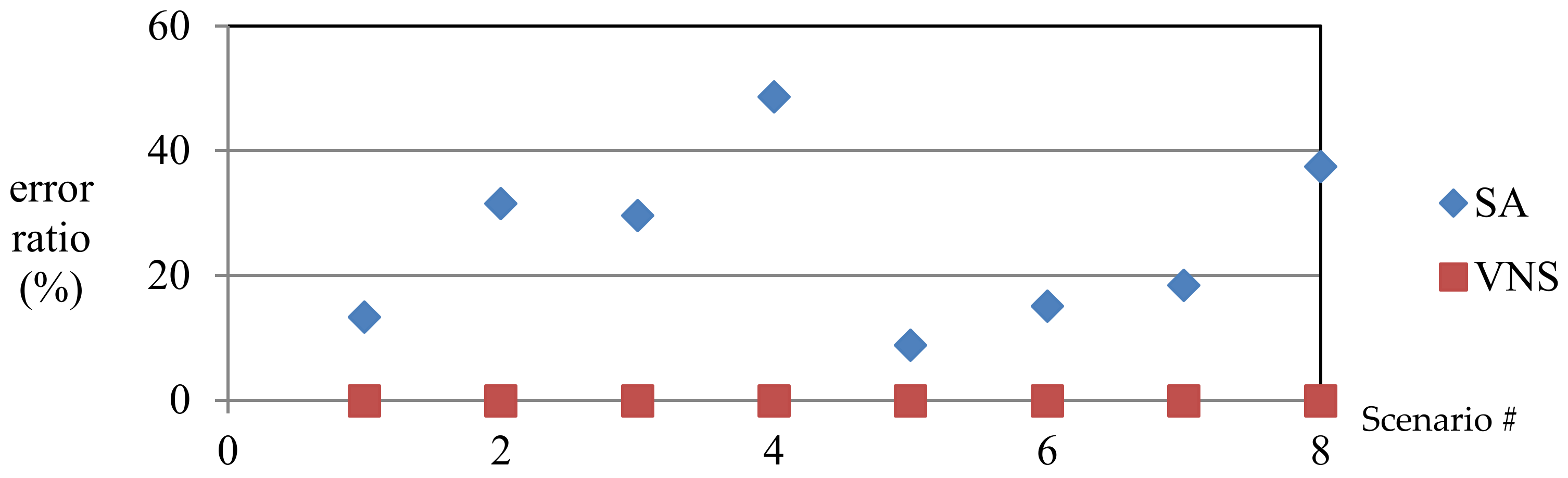
Five initial order-batching methods are proposed; we further tested these solutions under eight scenarios and with three random seeds. The results revealed that the BFD method yielded favorable results under all scenarios. In addition, the chain length and perturbation factors of the solutions were considered. Finally, the SA and VNS algorithms were incorporated into the solution comparisons. The algorithm processes were divided into two stages: The first stage involved batching, and the second stage involved optimizing the route. Under various scenarios, the VNS algorithm returned more favorable solutions than did the SA algorithm; moreover, the VNS algorithm demonstrated a faster solving speed. By contrast, the SA algorithm exhibited a slow solving speed in large-scale problems and converged slowly.

This study takes the conventional rectangular warehouse layout as an example layout. However, in practical applications, the layouts of almost all warehouses are different. This does not affect the algorithm design of order batching, but only affects the optimal picking distance between any two points in the order-picking-route problem. The distance between any two points can be obtained by calculating the minimum distance between any two points in advance, that is, it does not affect the implementation of the overall algorithm. Therefore, in practical applications, for the retail industry, small- and medium-sized online shopping retail warehouses or traditional retail warehouse can utilize this two-stage algorithm for their daily routine picking jobs. As for the picking of large objects in practice, the picking efficiency can be measured over time by increasing the picking time of some picking points. The objective can be adjusted to the minimal picking time and the concept of the whole two-stage algorithm can still be applied.

In further studies, this topic could be divided into three aspects to discuss. First, some restrictions could be loosened in the problem. For example, the same order could be divided into different batches, the picking time could be used to measure the picking efficiency, and different types of picking container equipment could be considered. Secondly, more effective initial batching methods could be developed because a good initial batching solution can save much computational time. Some metaheuristic algorithms newly developed in recent years, such as the spotted hyena optimizer (SHO) and dandelion algorithm (DA), could be developed for this problem because of their simple steps and fast computation. Finally, more warehouse layouts could be covered in the study in order to test the pros and cons of the proposed algorithm.