Modeling and I-NSGA-III-VLC Solution of Aircraft Equipment Rotation and Echelon Usage under Uncertainty

Featured Application

In this study, an effective multi-objective optimization method (I-NSGA-III-VLC) is proposed and applied to the rotation and echelon usage problem of aircraft equipment under uncertainty, proving the effectiveness of the method.

Abstract

Optimizing the aircraft equipment usage scheme of different units according to their task intensity has great significance in improving aircraft reliability and health management. This paper studied the modeling and solving methods of the rotation and echelon usage problems of aircraft equipment measured by dual-life indexes, one of which cannot be controlled. In order to maximize the waste rate of the rotation quantity, echelon uniformity index, life matching index and life utilization index, a decision-making model of the equipment rotation and echelon usage problem under uncertainty was constructed, and an improved NSGA-III with a variable length chromosome was proposed. An improved segmented coding method and operators were proposed, and the repeated individual control mechanism was used to improve the population diversity. When the scale of the problem was large, this method could search a wider range in a short time and obtain more feasible solutions, which verified the feasibility of this method.

1. Introduction

The life of many pieces of aircraft equipment is measured by two indexes, namely calendar life (CL) and working life (WL), and this type of equipment is called dual-life equipment (hereinafter referred to as equipment). Similar to aviation-guided munitions, the “power on time” is the working life of aviation-guided munitions.

The specified available calendar life for maintenance is called the stage calendar life, and the specified available working life for maintenance is called the stage working life. The calendar life is gradually consumed over time regardless of whether the task is executed or not, and it is uncontrollable, while the working life is only consumed by the execution of the task, which is controllable. In the actual usage process, the number of tasks for each unit and the number of pieces of equipment rotated between units are uncertain due to the lack of a rotation and echelon usage scheme formulation method. The scheme selection method is random and subjective [1], resulting in the fact that when the calendar life of the equipment stage is exhausted, its working life only consumes 40~60% of its stage working life [2], and the working life is seriously wasted and the echelon state is difficult to control. In the case of no rotation, due to the different equipment states and working intensities of different units, the life utilization index and life matching index of equipment are greatly different. Therefore, an effective rotation and echelon usage control method has an important role in solving the problems associated with echelon uniformity, life utilization and the life-matching degree of each unit.

Liu [3] established a set of comprehensive evaluation indexes, including working life combat-readiness reserves and echelon-uniformity indexes. However, these indexes cannot adapt to the situation of considering calendar life, and cannot control the echelon status. Zhang [4] proposed an improved echelon usage diagram method, which is concise and intuitive. Zhou et al. [5] proposed a formation and control method of motorcycle working life echelon reserves using SAA to formulate a usage and repair plan of a motorcycle. For assignment problems, Dorterler [6] proposed a new genetic algorithm with agent-based crossover for the generalized assignment problem, but it is based on the idea that each task should be assigned to one agent only. Fu et al. [7] studied the uncertain multi-objective assignment problem, in which the number of tasks each person undertakes is uncertain, but each task can only be undertaken by one person. Xiong [8] solved the assignment problem of multiple people participating in a task with a new generalized nonlinear integer programming model and verified its effectiveness through an example. Ding [9,10] proposed an α-optimistic uncertain assignment model, but this model has the limitations of low efficiency and large storage space requirements.

2. Problem Description and Modeling

2.1. Problem Description

In the case of rotation, the echelon usage problem of equipment belongs to the uncertain assignment problem. The characteristics of this kind of assignment problem are that the amount of equipment in each rotation is uncertain, the quantity of tasks that each equipment can undertake is uncertain and the objective function result is uncertain before the decision matrix is determined.

According to the remaining-life data of equipment and task quantity in different units, the arrangement of the equipment to be rotated is calculated first, followed by the performance of a task of $a$ months, where $a$ is a positive integer, aiming at maximizing the average working-life echelon-uniformity index, the average calendar-life- and working-life-matching index, the average life-utilization-rate index, and the waste rate-of-rotation-quantity index. The result is the number of pieces of equipment rotated by each unit and the quantity of tasks completed by each piece equipment each month.

The average working-life echelon uniformity refers to the average value of the working-life echelon uniformity of each unit, hereinafter referred to as the average echelon uniformity. The average calendar-life- and working-life-matching-degree index refer to the average value of the calendar-life- and working-life matching-degree index of each unit, hereinafter referred to as the average matching-degree index. The average life-utilization rate refers to the average value of the life-utilization rate of each unit, hereinafter referred to as the average utilization-rate index. The waste rate-of-rotation-quantity index refers to the ratio of the unused rotation equipment quantity to the maximum equipment rotation quantity of all units.

2.2. Problem Assumptions

• Assumption 1: There is complete interchangeability between the equipment;
• Assumption 2: The quantity of tasks per month of each unit is fixed;
• Assumption 3: The quantity of equipment required for each unit is fixed;
• Assumption 4: The working-life consumption per task is fixed;
• Assumption 5: The calendar life of each piece of equipment is an integer, with the unit of months;
• Assumption 6: There is no limit to the number of times each piece of equipment can be used every month;
• Assumption 7: Equipment failure is not considered during rotation and usage;
• Assumption 8: The upper limit of the amount of equipment in each rotation is determined;
• Assumption 9: The calendar life consumption caused by rotation is negligible.

2.3. Problem Inputs

• Task quantity sequence every month of each unit $U$;
• Quantity of equipment required for each task $v$;
• Working-life consumption per task $w$;
• Stage working life of equipment $MWL$;
• Stage calendar life of equipment $MCL$;
• Task time range $a$;
• Maximum quantity of equipment for each rotation $g$;
• Equipment quantity sequence of each unit $N$;
• Unit quantity $c$.

2.4. Problem Ouputs

• Equipment number of each rotation;
• Number of pieces of equipment used for each task.

2.5. Mathematical Model

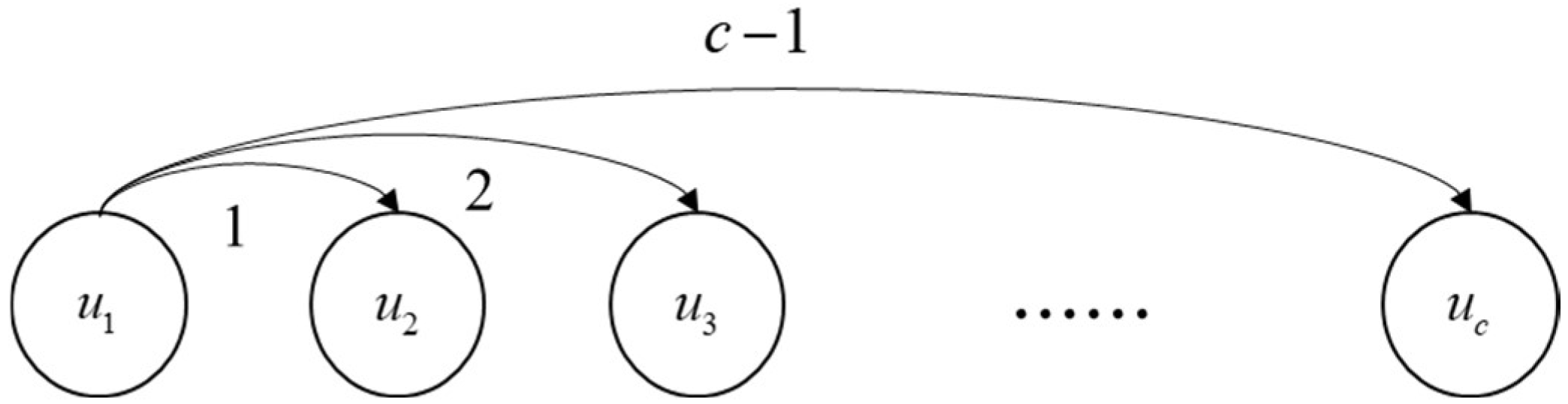
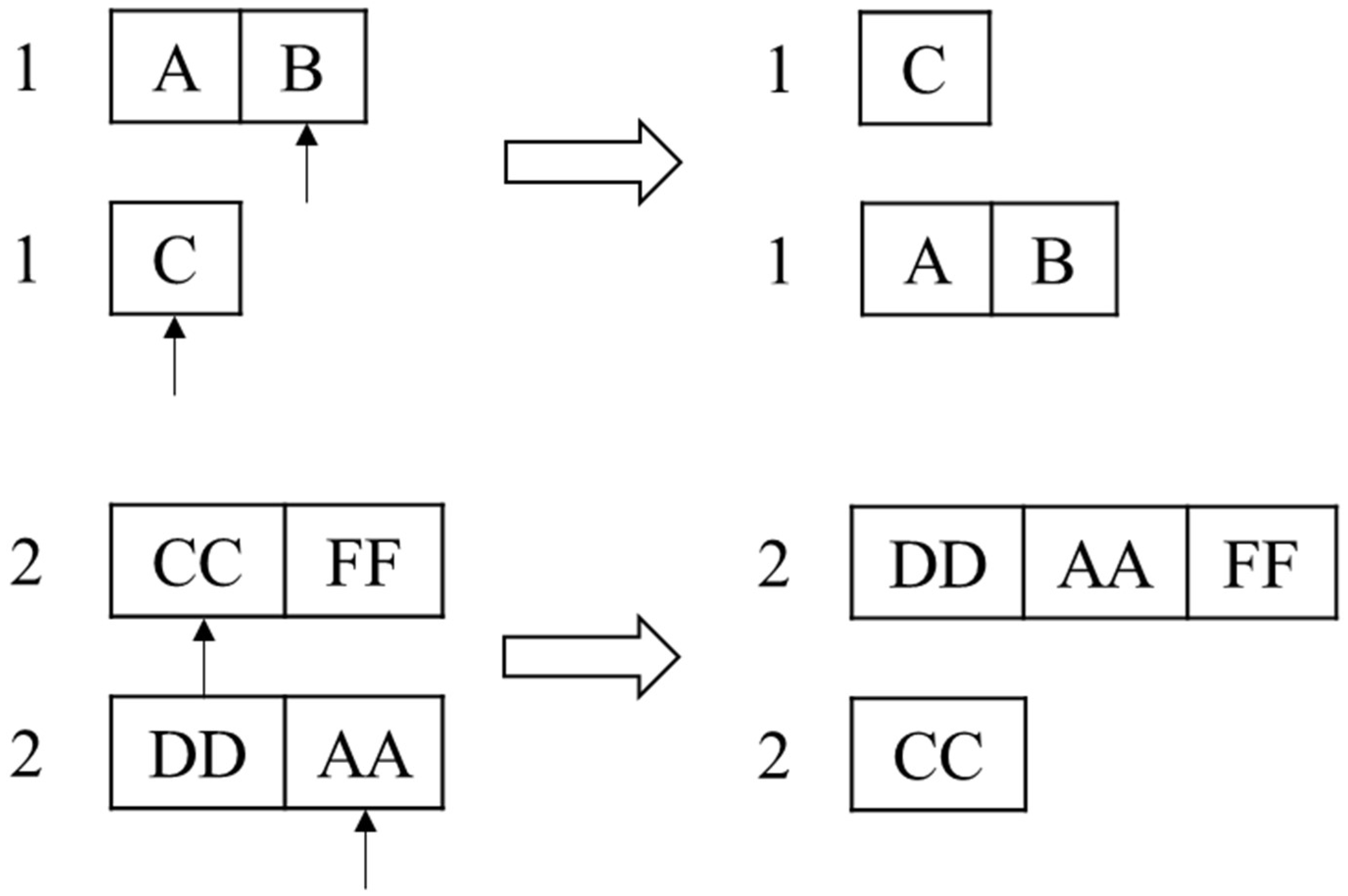
Taking unit $u_1$ as an example, when rotating from $u_1$ to other units, the rotation number is $c-1$, and the rotation process is shown in Figure 1.

The decision matrix is divided into two parts.

Let us introduce the 0-1 variable $x_{i,j}(i=1,2,\dots ,c-1,j=S_{1,1},S_{1,2},\dots ,S_{1,N_1},c\ge 2)$, where $S_1$ is the equipment number sequence of $u_1$, $N_1$ is the equipment quantity of $u_1$. By analogy, the 0-1 variable is also introduced for other units to build a rotation decision matrix. The selected equipment is moved to the corresponding unit, and the equipment numbers of the current unit and the corresponding unit are updated. $S^{\prime }$ is the updated equipment number sequence of each unit and $N^{\prime }$ is the updated equipment quantity sequence of each unit.

$$x_{i,j}=\left\{\begin{array}{l}0 S_i is not selected in j_{th} rotation\\ 1 S_i is selected in j_{th} rotation\end{array}\right.$$

Let us introduce the 0-1 variable $y_{i,j}=(i=1,2,\dots ,a\ast U_1;j=1,2,\dots ,n)$, where $U_1$ is the task quantity of $u_1$. By analogy, the 0-1 variable is also used for other units to construct the task decision matrix and update the working life of the selected equipment.

$$y_{i,j}=\left\{\begin{array}{l}0 S_i^{\prime } is not selected in j_{th} task\\ 1 S_i^{\prime } is selected in j_{th} task\end{array}\right.$$

Next, let us establish the rotation decision matrix, $X$, and task decision matrix, $Y$, of $u_1$, as shown in

Table 1. Construction rotation decision matrix $X$ of $u_1$.

	Equipment Number	${\mathit{S}}_{1,1}$	${\mathit{S}}_{1,2}$	$\cdots$	${\mathit{S}}_{1,{\mathit{N}}_1-1}$	${\mathit{S}}_{1,{\mathit{N}}_1}$
Rotation Time
$1$		$x_{1,1}$	$x_{1,2}$	$\cdots$	$x_{1,N_1-1}$	$x_{1,N_1}$
$2$		$x_{2,1}$	$x_{2,2}$	$\cdots$	$x_{2,N_1-1}$	$x_{2,N_1}$
$⋮$		$⋮$	$⋮$	$\cdots$	$⋮$	$⋮$
$c-2$		$x_{c-2,1}$	$x_{c-2,2}$	$\cdots$	$x_{c-2,N_1-1}$	$x_{c-2,N_1}$
$c-1$		$x_{c-1,1}$	$x_{c-1,2}$	$\cdots$	$x_{c-1,N_1-1}$	$x_{c-1,N_1}$

and

Table 2. Construction task decision matrix $Y$ of $u_1$.

	Equipment Number	${\mathit{S}}_{{}_{1,1}}^{\prime }$	${\mathit{S}}_{1,2}^{\prime }$	$\cdots$	${\mathit{S}}_{1,{\mathit{N}}_1^{\prime }-1}^{\prime }$	${\mathit{S}}_{1,{\mathit{N}}_1^{\prime }}^{\prime }$
Task
$1$		$y_{1,1}$	$y_{1,2}$	…	$y_{1,N_1^{\prime }-1}$	$y_{1,N_1^{\prime }}$
$2$		$y_{2,1}$	$y_{2,2}$	…	$y_{2,N_1^{\prime }-1}$	$y_{2,N_1^{\prime }}$
$⋮$		$⋮$	$⋮$	$\cdots$	$⋮$	$⋮$
$a\ast U_1-1$		$y_{a\ast U_1-1,1}$	$y_{a\ast U_1-1,2}$	$\cdots$	$y_{a\ast U_1-1,N_1^{\prime }-1}$	$y_{a\ast U_1-1,N_1^{\prime }}$
$a\ast U_1$		$y_{a\ast U_1,1}$	$y_{a\ast U_1,2}$	$\cdots$	$y_{a\ast U_1,N_1^{\prime }-1}$	$y_{a\ast U_1,N_1^{\prime }}$

.

$$X=\left(\begin{array}{ccc}{x}_{1,1}& \dots & x_{1,N_1}\\ ⋮& \ddots & ⋮\\ x_{c-1,1}& \cdots & x_{c-1,N_1}\end{array}\right)$$

$$Y=\left(\begin{array}{ccc}{y}_{1,1}& \dots & y_{1,N_1^{\prime }}\\ ⋮& \ddots & ⋮\\ y_{a\ast U_1,1}& \cdots & y_{a\ast U_1,N_1^{\prime }}\end{array}\right)$$

Constraints:

$$s.t.\left\{\begin{array}{l}{\displaystyle \sum _{j=1}^{N_1}{x}_{i,j}}\le g\\ 0\le {\displaystyle \sum _{i=1}^{a\ast U_1}{y}_{i,j}\le T_{1,j}=\left\{\begin{array}{l}Floor(\frac{W{L}_{1,j}}{w})\hspace{1em}\hspace{1em}\hspace{1em}Floor(\frac{W{L}_{1,j}}{w})\le U_1\ast C{L}_{1,j}\\ U_1\ast C{L}_{1,j}\hspace{1em}\hspace{1em}\hspace{1em}\hspace{1em}Floor(\frac{W{L}_{1,j}}{w})>U_1\ast C{L}_{1,j}\end{array}\right.}\\ {\displaystyle \sum _{i=1}^{c-1}{x}_{i,j}}\le 1\\ {\displaystyle \sum _{i=1}^{N_1^{\prime }}{y}_{i,j}}=v\end{array}\right.$$

Update data:

$$\left\{\begin{array}{l}W{L}^{\prime }{}_{1,j}=W{L}_{1,j}-w\ast {\displaystyle \sum _{i=1}^{a\ast U_1}{x}_{i,j}}\\ C{L}^{\prime }{}_{1,j}=C{L}_{1,j}-a\end{array}\right.$$

$T_{i,j}$ are the remaining usable times of $S_{i,j}^{\prime }$, where $W{L}^{\prime }$ and $C{L}^{\prime }$ are the updated remaining working life sequence and calendar life sequence. The fitness functions of this problem are the average echelon-uniformity function of each unit, average life-matching function of each unit, average utilization function and rotation-quantity waste function.

1.

The average echelon-uniformity function, $F_1$.

The improved echelon-uniformity function, $Q_1$, of $u_1$ is shown in Formula (1)

$$Q_1=\left(1-\sqrt{\frac{{\displaystyle \sum _{i=1}^{N_1^{\prime }-1}}{\left(U{L}_{1,i+1}-U{L}_{1,i}-\frac{e_1}{{\left(N_1^{\prime }\right)}^2}\right)}^2+{\left(U{L}_{1,1}+e_1-U{L}_{1,N_1}-\frac{e_1}{{\left(N_1^{\prime }\right)}^2}\right)}^2}{\left(N_1^{\prime }-1\right){\left(\frac{e_1}{{\left(N_1^{\prime }\right)}^2}\right)}^2+{\left(e_1-\frac{e_1}{{\left(N_1^{\prime }\right)}^2}\right)}^2}}\right)\times 100\%$$

(1)

This is continued for other units to acquire $F_1=\frac{{\displaystyle \sum _{i=1}^c{Q}_i}}{c}$.

$U{L}_1$ is the sequence of sorted $W{L}_1^{\prime }$ in ascending order according to the $C{L}_1^{\prime }$ of $u_1$. Its purpose is to increase the working life along the direction of increasing calendar life. $e_1$ is the maximum value in $U{L}_1$, and $N_1^{\prime }$ is the quantity of equipment of $u_1$.

2.

The average life-matching function, $F_2$.

The life-matching function, $Z_1$, of $u_1$ is shown in Formula (2)

$$\begin{array}{l}{Z}_1=\left(1-\frac{{\displaystyle \sum _{i=1}^{N_1^{\prime }}{H}_{1,i}}}{N_1^{\prime }\ast V_1}\right)\\ H_{1,i}=\left\{\begin{array}{l}\left|\frac{MWL-W{L}^{\prime }{}_{1,i}}{MCL-C{L}^{\prime }{}_{1,i}}-\frac{MWL}{MCL}\right| C{L}^{\prime }{}_i\ne MCL\\ \left|(MWL-W{L}^{\prime }{}_{1,i})-\frac{MWL}{MCL}\right| C{L}^{\prime }{}_i=MCL\end{array}\right.\end{array}$$

(2)

This is continued for other units to acquire $F_2=\frac{{\displaystyle \sum _{i=1}^c{Z}_i}}{c}$.

$H_{1,i}$ is the absolute value of the difference between the updated used working life and the used calendar life ratio and the ideal ratio of each equipment. When $C{L}_{1,i}^{\prime }=MCL$, the used working life of the equipment is calculated as a ratio.

3.

The average utilization function, $F_3$.

It is defined that the standard for equipment to enter into consumption is that the working life must be less than 3 h or the calendar life must be less than 1 month. When the equipment reaches the consumption standard, it can be considered that the utilization rate is 100%. The process is as follows:

For $u_1$, define $k_{1,1}:=0$, $k_{1,2}:=0$, $RW{L}_1:=0$, $RC{L}_1:=0$.

Traverse the updated data.

When $C{L}^{\prime }{}_{1,i}:=0$, $k_{1,1}:=k_{1,1}+1$;

When $W{L}^{\prime }{}_{1,i}\ge w$, $RW{L}_1:=RW{L}_1+W{L}^{\prime }{}_{1,i}$;

When $W{L}^{\prime }{}_{1,i}<w$, $RW{L}_1:=RW{L}_1+0$;

When $W{L}^{\prime }{}_{1,i}<w$, $k_{1,2}:=k_{1,2}+1$, $RC{L}_1:=RC{L}_1+C{L}^{\prime }{}_{1,i}$.

The utilization function of $u_1$ is shown in Formula (3).

$$R_1=\left\{\begin{array}{l}\frac{\frac{k_{1,1}\ast MWL-RW{L}_1}{k_{1,1}\ast MWL}+\frac{k_{1,2}\ast MCL-RC{L}_1}{k_{1,2}\ast MCL}}{2}\ast 100\%\hspace{1em}\hspace{1em}\hspace{1em} k_{1,1}>0\&k_{1,2}>0\\ \frac{k_{1,1}\ast MWL-RW{L}_1}{k_{1,1}\ast MWL}\ast 100\%\hspace{1em}\hspace{1em}\hspace{1em}\hspace{1em}\hspace{1em}\hspace{1em}\hspace{1em} k_{1,1}>0\&k_{1,2}=0\\ \frac{k_{1,2}\ast MCL-RC{L}_1}{k_{1,2}\ast MCL}\ast 100\%\hspace{1em}\hspace{1em}\hspace{1em}\hspace{1em}\hspace{1em}\hspace{1em}\hspace{1em} k_{1,2}>0\&k_{1,1}=0\end{array}\right.$$

(3)

$k_{1,1}$ is the quantity of equipment with an exhausted calendar life of $u_1$, $k_{1,2}$ is quantity of equipment with an exhausted calendar life of $u_1$, $RW{L}_1$ is the sum of the remaining working life of the equipment with an exhausted calendar life after updating $u_1$, and $RC{L}_1$ is the sum of the remaining calendar life of the equipment with an exhausted working life after updating $u_1$.

This is continued for other units to acquire $F_3=\frac{{\displaystyle \sum _{i=1}^c{R}_i}}{c}$.

4.

The rotation-quantity waste function, $F_4$.

The transportation cost and risk level caused by rotation can be replaced by the equipment rotation quantity. In order to reduce the equipment transportation cost and risk caused by rotation, the number of rotating pieces of equipment should be as small as possible.

Let us assume that the number of pieces of equipment rotated from a certain unit at each time cannot exceed $g$, the rotation phase can be divided into from $u_1$ to $u_2$, from $u_1$ to $u_3$,…, from $u_1$ to $u_c$,…, and from $u_c$ to $u_{c-1}$, where the total time of rotations is $c\ast (c-1)$, and the maximum quantity of rotations is $c\ast (c-1)\ast g$. Let us assume that the rotation quantity represented by an individual chromosome is $P$, the rotation-quantity waste rate function of the individual $F_4$ is shown in Formula (4).

$$F_4=\frac{c\ast (c-1)\ast g-P}{c\ast (c-1)\ast g}$$

(4)

Aiming at the multi-objective assignment problem with an uncertain rotation quantity, with the task quantity completed by each equipment under the conditions of rotation, this paper constructed a decision-making model for the rotation and echelon usage of dual-life equipment and proposed an improved NSGA-III method with a variable length chromosome (I-NSGA-III-VLC) to solve it. This method can obtain a variety of optimization schemes in a relatively short time. Through scheme screening, the problem of poor working-life echelon status, low matching between calendar life and working life and the low utilization of the working life of equipment in different units can be solved to a certain extent with as few rotations as possible.

3. Principle of I-NSGA-III-VLC Method

Optimizing the equipment echelon uniformity, life-matching degree, life utilization and rotation-quantity waste rate at the same time is a high-dimensional multi-objective optimization problem. Deb proposed a fast, non-dominated-sorting genetic algorithm based on reference points (NSGA-III) [11], which replaced the congestion by associating the reference points, and solved the problem of high-dimensional objective optimization. Many scholars have solved high-dimensional multi-objective optimization problems based on the above algorithms, including the multi-objective classification problem [12], reservoir flood-control-operation problem [13], resource-allocation problem [14,15,16], location-routing problem [17,18,19,20], high-dimensional target power-flow-optimization problem of a power system [21,22], etc.

The feasible region of many problems is uncertain in real life. Many scholars [23,24,25,26,27,28,29] have improved the NSGA-III-VLC according to the characteristics of the problem. In the formulation of the equipment usage plan considering rotation, because the quantity of rotation will affect the rotation cost and risk, the length of the chromosome also affects the decision-making. In this paper, the chromosome-coding method, crossover operator, mutation operator and repetitive individual control operator were improved according to the characteristics of the problem. The specific improvement contents are shown from Section 3.1, Section 3.2, Section 3.3, Section 3.4 and Section 3.5.

3.1. Variable Length Cegment Hybrid Coding Method

Due to the need for considering the rotation between different units, the chromosome-coding method needs to be changed to distinguish different units. The rotation stage is placed before the task stage. This paper adopted the variable length and hybrid segmented-coding methods. Let us add a number “prefix” before each rotation, such as 1, 2, …, $c\ast (c-1)$. Therefore, the shortest chromosome length at the rotation stage is $c\ast (c-1)$, and the maximum quantity of equipment for each rotation is $g$. Therefore, the longest chromosome length is $c\ast (c-1)\ast (g+1)$.

After the rotation phase, according to the task intensity sequence $U$ and $V$ of each unit, according to the unit quantity, let us add a number “prefix” before each unit task, such as $c\ast (c-1)+1$,$c\ast (c-1)+2$,…,$c^2$. Therefore, the total length of chromosomes in the task phase is ${\displaystyle \sum _{i=1}^c{N}_i^{\prime }\ast a}+c$.

Each coding segment is divided by a digital “prefix”. With this coding method, we can not only distinguish each unit but also cross and mutate under the same “prefix”. The range of crossover and mutation is reduced, and it is easy to control the chromosome length. The chromosome initialization process is shown below.

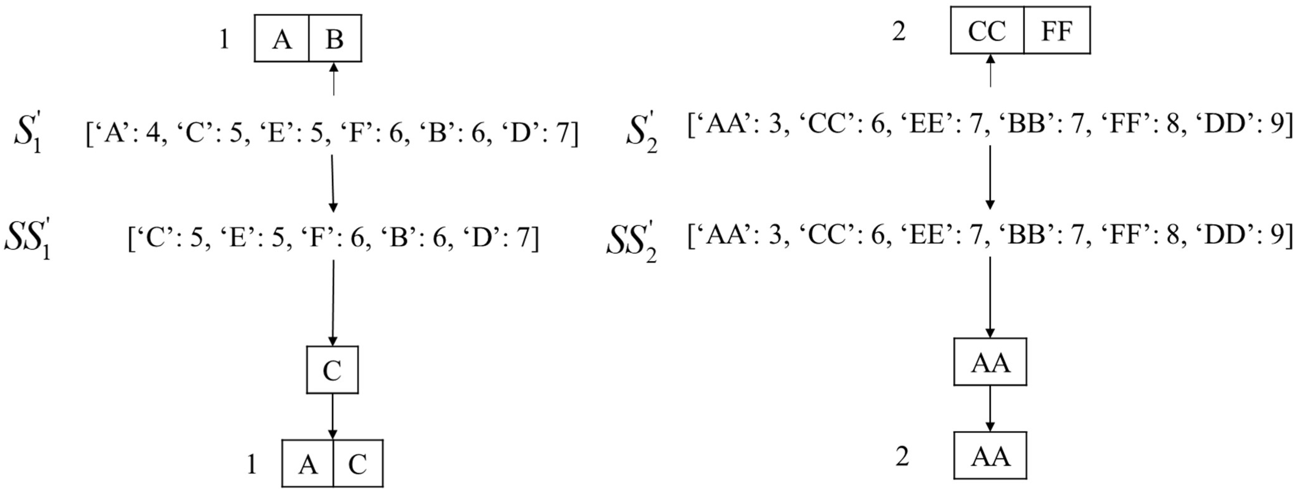
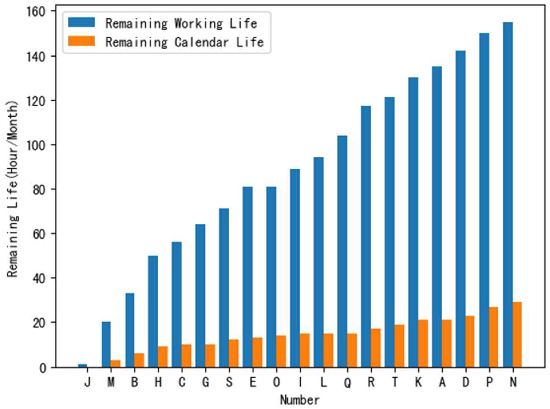
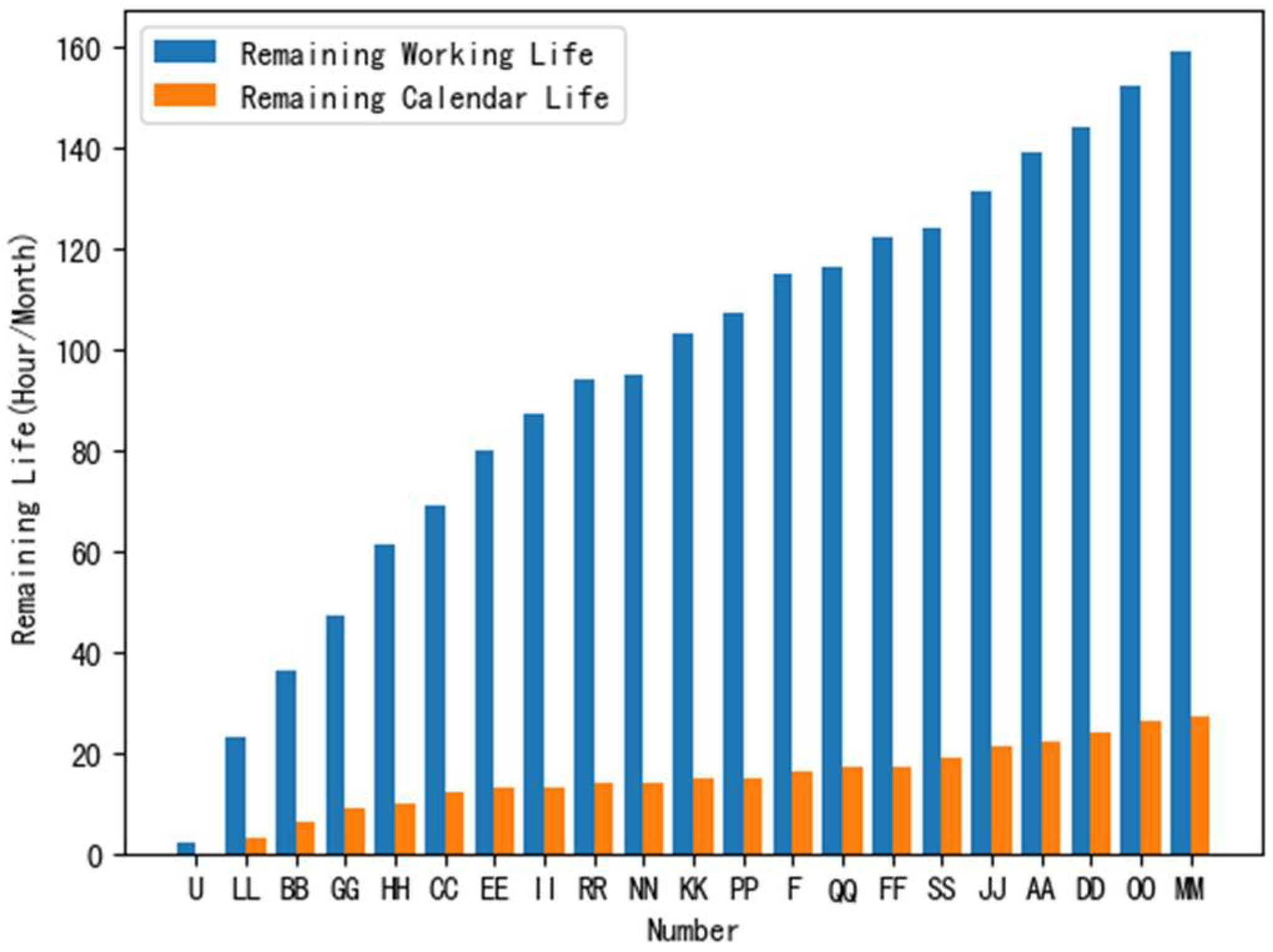
Step 1: Arrange all equipment numbers $S_i$ and remaining usable times $T$ in each unit to form a sequence in $S_i^{\prime }$ in the format of “Number: Remaining Usable Times”. Like all equipment numbers, $S_1^{\prime }$ of $u_1$ is $S_1^{\prime }=$ [‘A’: 4, ‘C’: 5, ‘E’: 5, ‘F’: 6, ‘B’: 6, ‘D’: 7], and like all equipment numbers, $S_2^{\prime }$ of $u_2$ is $S_2^{\prime }=$ [‘AA’: 3, ‘CC’: 6, ‘EE’: 7, ‘BB’: 7, ‘FF’: 8, ‘DD’: 9].

Step 2: Adopt a segmental coding method where there are $c\ast (c-1)$ coding segments in the rotation phase, and the shortest length of each coding segment is 1 and the longest is $g+1$. Assume $c=2$, $g=3$. Randomly select $l_1$ equipment from $u_1$ and randomly select $l_2$ equipment from $u_2$,$0\le l_1,l_2\le g$, where the equipment number and “prefix” together constitute the code segment, i.e., [1, ‘A’, ‘B’, 2, ‘CC’, ‘FF’]. This indicates that the first rotation is to rotate the equipment numbered ‘A’ and ‘B’ in $u_1$ to $u_2$, and the second rotation is to rotate the equipment numbered ‘CC’ and ‘FF’ in $u_2$ to $u_1$.

Add ‘A’ and ‘B’ to $u_1$ according to the remaining usable times, delete them in $u_2$, add ‘CC’ and ‘FF’ to $u_2$ according to the remaining usable times, delete them in $u_1$, update $S_1^{\prime }$ and $S_2^{\prime }$, and obtain $S_1^{″}=$ [‘C’: 5, ‘E’: 5, ‘F’: 6, ‘CC’: 6, ‘D’: 7, ‘FF’: 8] and $S_2^{″}=$ [‘AA’: 3, ‘A’: 4, ‘B’: 6, ‘EE’: 7, ‘BB’: 7, ‘DD’: 9].

Step 3: In the task phase, the order of executing the task of the equipment is not considered in the same coding segment, but it cannot be reused. Gene $j$ can be reused in different coding segments, but the number of repetitions cannot exceed the corresponding remaining usable times. The total length of code in a task stage is $U_i\ast v$. Assume $U_1=2$, $U_2=1$, $v=4$, initialize the chromosome, select $v$ equipment from $u_1$ as a group, repeat $U_1$ times and select $v$ equipment from $u_2$ as a group, repeat $U_2$ times, such as [3, [‘CC’, ‘C’, ‘E’, ‘F’], [‘C’, ‘E’, ‘FF’, ‘D’], 4, [‘AA’, ‘B’, ‘EE’, ‘DD’]]. This coding method can be directly interpreted as selecting the equipment to complete the task. The segmented real-number coding conforms to the practical significance, and it is easy to control the upper limit of usage times.

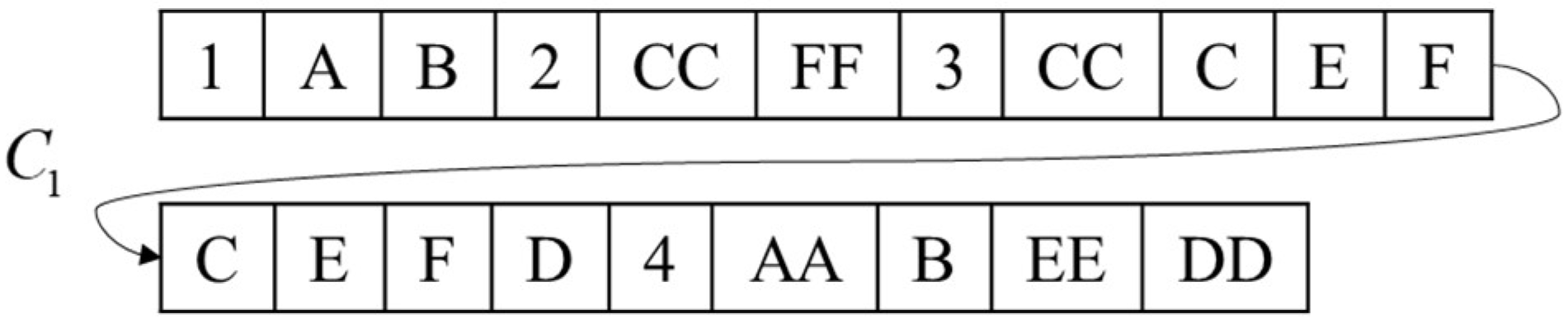
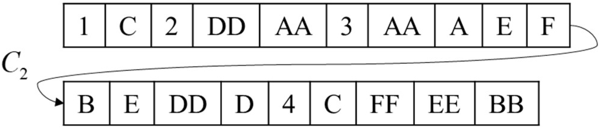
Step 4: Combine the chromosomes of the two stages to acquire $C_1=$ [1, ‘A’, ‘B’, 2, ‘CC’, ‘FF’, 3, [‘CC’, ‘C’, ‘E’, ‘F’], [‘C’, ‘E’, ‘FF’, ‘D’], 4, [‘AA’, ‘B’, ‘EE’, ‘DD’]]. By the same token, $C_2=$ [1, ‘C’, 2, ‘DD’, ‘AA’, 3, [‘AA’, ‘A’, ‘E’, ‘F’], [‘B’, ‘E’, ‘DD’, ‘D’], 4, [‘C’, ‘FF’, ‘EE’, ‘BB’]]. $C_1$ is shown in Figure 2, and $C_1$ is shown in Figure 3.

3.2. Population Initialization

Step 1: Population size $M$, $pop=[ ]$, $s:=0$, equipment numbers $S^{\prime }$, such as $S_1^{\prime }=$ [‘A’: 4, ‘C’: 5, ‘E’: 5, ‘F’: 6, ‘B’: 6, ‘D’: 7] and $S_2^{\prime }=$ [‘AA’: 3, ‘CC’: 6, ‘EE’: 7, ‘BB’: 7, ‘FF’: 8, ‘DD’: 9];

Step 2: Initialize chromosome $C$, acquire $S_1^{″}$ and $S_2^{″}$ and calculate the usage time $p$ of each equipment number in the chromosome in the format of “Number: Usage Times”. For example, $p_1$ of $C_1$ is [‘C’: 2, ‘E’: 2, ‘F’: 1, ‘CC’: 1, ‘D’: 1, ‘FF’: 1] and $p_2$ of $C_1$ is [‘AA’: 1, ‘B’: 1, ‘EE’: 1, ‘DD’: 1];

Step 3: Traverse the number in $p_i$. If the usage time of the number is greater than the remaining usable time of the corresponding number in $S_1^{″}$, return to Step 2. Otherwise, enter Step 4.

Step 4: Add $C$ to the $pop$, where $s:=s+1$. If $s<M$ return to Step 2. Otherwise, the population initialization is completed.

3.3. Crossover Operator

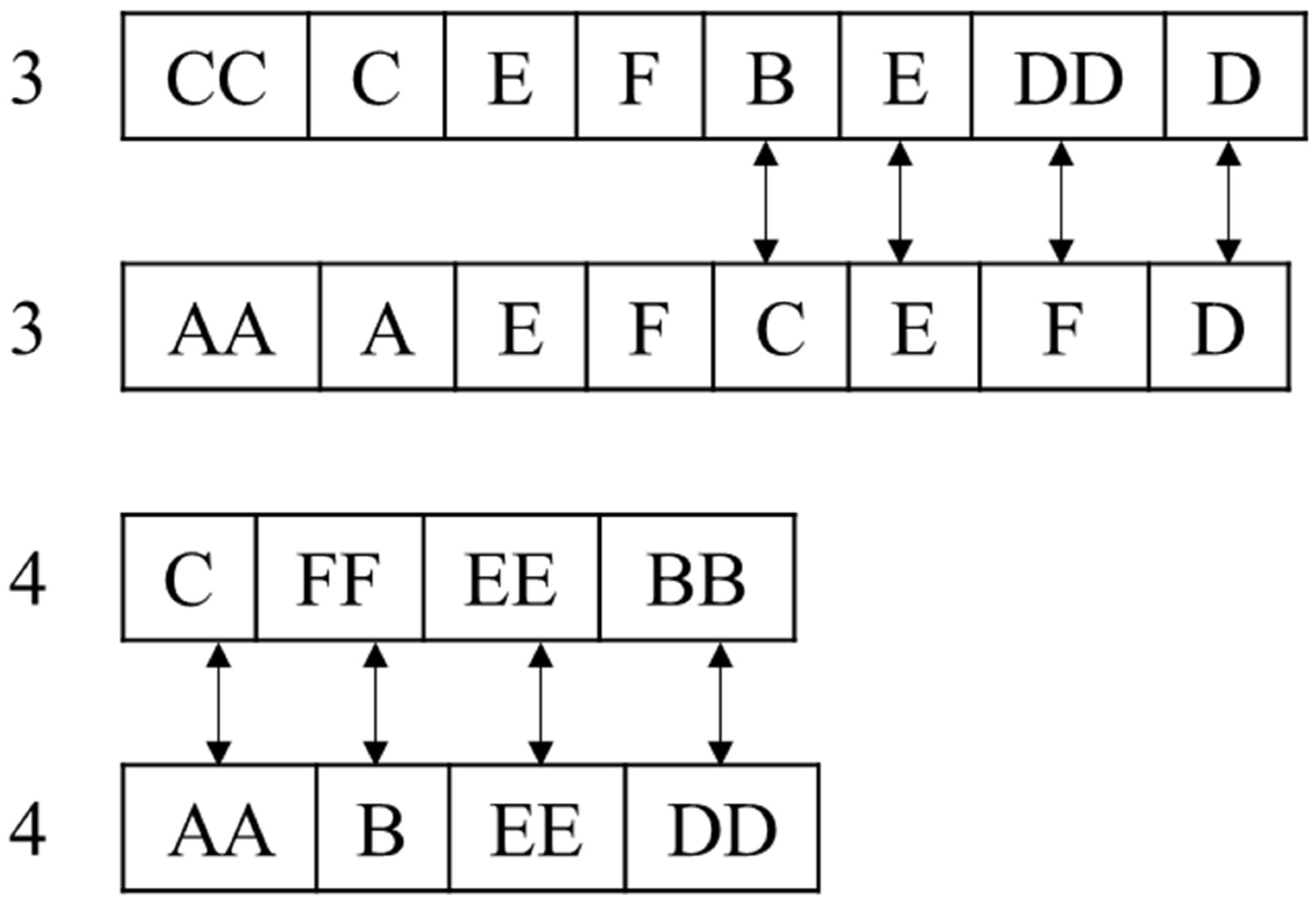
For different coding stages, the ectopic single point crossover method was adopted in the rotation stage, and the two-point crossover method was adopted in the task stage. The crossover operator steps are as follows.

Step 1: Given the crossover rate $p_c$, $0\le p_c\le 1$, the new population size is $M$, where $new\_pop=[ ]$, and $s:=0$.

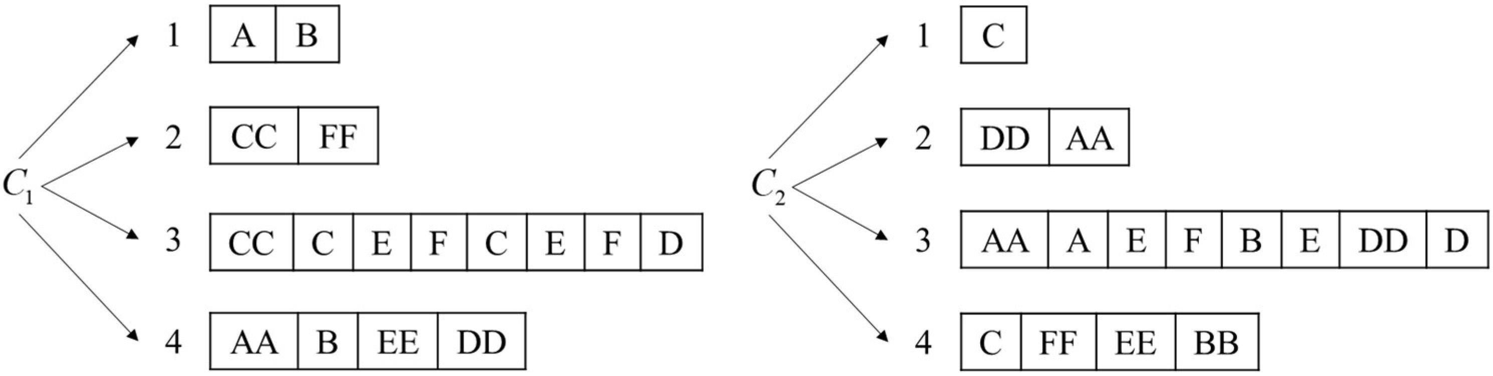
Step 2: Select two parent individuals and define $coun{t}_1:=0$ and $coun{t}_2:=0$. The paternal chromosomes are segmented according to the number “prefix”, as shown in Figure 4.

Step 3: Combine the split parent individuals according to the same “prefix”. Because the first $c\ast (c-1)$ combinations belong to the rotation stage, the length of coding segments may be different, so the heterotopic single point crossover method is adopted.

For the code segment combination in the rotation stage:

Step 4: Randomly select two points $nu{m}_{1,j}$ and $nu{m}_{2,j}$, where $nu{m}_{i,j}$ is the point selected from the coding segment with “prefix” $j$ of the parent $i$. In addition, $0\le nu{m}_{1,j}\le le{n}_{1,j}\le g$, $0\le nu{m}_{2,j}\le le{n}_{2,j}\le g$, $0\le le{n}_{1,j}-nu{m}_{1,j}+nu{m}_{2,j}\le g$, and $0\le le{n}_{2,j}-nu{m}_{2,j}+nu{m}_{1,j}\le g$, where $le{n}_{i,j}$ is the length of the coding segment of the parent $i$ with “prefix” $j$.

Step 5: Generate a random number $r_c$ between 0 and 1. If $r_c\le p_c$ and $coun{t}_1<10$, crossover the first $nu{m}_{1,j}$ genes of the coding segment with $j$ as the “prefix” in parent1 and the first $nu{m}_{2,j}$ genes of the coding segment with $j$ as the “prefix” in parent2. $coun{t}_1:=coun{t}_1+1$, generate crossover results, as shown in Figure 5, and enter Step 6. If $p_c<r_c$, do not crossover, return Step 4. If $coun{t}_1=10$, the parent individuals will be preserved in the new population.

The specific steps of modifying operator 1 are as follows.

Step 6: Calculate the repetitions $g_i$ of each number after crossover in the format “Number: Repetitions”. Iterate through the numbers in $g_i$. If the repetitions of the number are 1 and the set of numbers is a subset of the number $S_i^{\prime }$, acquire $S_i^{″}$ and enter Step 7. Otherwise, return to Step 10.

For the code segment combination in the task stage:

Step 7: Adopt the method of two-point crossing and randomly select two points, $po{t}_1$ and $po{t}_2$, where $po{t}_1<po{t}_2$, $po{t}_1\%v=0$ and $po{t}_2\%v=0$.

Step 8: Generate a random number $r_c^{\prime }$ between 0 and 1. If $r_c^{\prime }\le p_c$ and $coun{t}_2<10$, exchange genes between two points, and if $coun{t}_2:=coun{t}_2+1$, generate crossover results, as shown in Figure 6, and enter Step 9. If $p_c<r_c^{\prime }$ and $coun{t}_2<10$ do not cross, return to Step 7. If $coun{t}_2=10$, the parent individuals are added to the new population, with $s:=s+2$.

The specific steps of modifying operator 2 are as follows.

Step 9: Calculate the number of repetitions $b_{i,j}$ of each character in each unit after crossover, where $i$ represents the individual number of the offspring after crossover, and $j$ represents the unit number in the format “Number: Quantity of Repetitions”. According to the different units, traverse the number in $b_{i,j}$. If the number of repetitions is less than the number of repetitions of the corresponding number in $S_i^{″}$ of the corresponding unit and the number of $b_{i,j}$ is a subset of $S_i^{″}$, enter Step 10. Otherwise, return to Step 7.

Step 10: Merge the cross results according to the “prefix” and add the results to the new population $new\_pop=[ ]$, where $s:=s+1$. If $s<M$, return to Step 2. If $s=M$, the crossover operator ends.

3.4. Mutation Operator

For different coding stages, the methods of gene mutation and gene length mutation are used, respectively. The steps of the mutation operator are as follows.

Step 1: Define the mutation rate $p_m$, $0\le p_m\le 1$.

Step 2: Select the parent individuals, define $coun{t}_1:=0$, $coun{t}_2:=0$, and divide the chromosome according to the number “prefix”.

For the combination of rotation stage:

Step 3: Randomly select two points $nu{m}_{1,j}$ and $nu{m}_{2,j}$, where $1\le nu{m}_1\le le{n}_1\le g$ and $1\le nu{m}_2\le le{n}_2\le g$.

Step 4: Generate a random number $r_m$ between 0 and 1. If $r_m\le p_m$, delete the number except $nu{m}_1$ in $S_1^{\prime }$ to get $S{S}_1^{\prime }$, and randomly select $0~g-nu{m}_1+1$ numbers from $S{S}_1^{\prime }$ to replace it. Similarly, delete the number except $nu{m}_2$ in $S_2^{\prime }$ to get $S{S}_2^{\prime }$, and randomly select $0~g-nu{m}_2+1$ numbers from $S{S}_2^{\prime }$ to replace it. Generate the mutation results, as shown in Figure 7, and enter Step 5. If $p_m<r_m$, do not generate the mutation, and return to Step 3.

Step 5: After obtaining the mutation results in the rotation stage, $S_i^{″}$ can be obtained according to the mutation results, such as $S_1^{″}=$ [‘AA’: 3, ‘E’: 5, ‘F’: 6, ‘B’: 6, ‘D’: 7] and $S_2^{″}=$ [‘A’: 4, ‘C’: 5, ‘CC’: 6, ‘EE’: 7, ‘BB’: 7, ‘FF’: 8, ‘DD’: 9].

For the code segment in the task phase:

Step 6: Traverse the code segment. If there is a number that does not belong to $S_i^{″}$, it will be replaced with the number in $S_i^{″}$ according to the number of the remaining usage time.

Step 7: Randomly select the code segment of the parent to generate a random number $r_m^{\prime }$ between 0 and 1.

Step 8: If $r_m^{\prime }\le p_m$, enter Step 9, otherwise, return to Step 7.

Step 9: Calculate the number of gene repetitions excluding coding segment $k_i$, and subtract $k_i$ from $S_i^{″}$ to acquire $q_i$.

Step 10: This coding segment is mutated into a gene segment generated by the set $q_i$, and no repeat genes are allowed.

This mutation operator ensures that the number repetitions of the chromosome gene after mutation is lower than the limit of the number repetitions, without using a new modifying operator, and improves the efficiency of the algorithm.

3.5. Population-Diversity-Preserving Operator

Step 1: Initialize the population, with the iteration number $epoch:=0$ and the diversity-keeping parameter $d$.

Step 2: Conduct the crossover, mutation and selection operators to generate a new generation of population, where $epoch:=epoch+1$.

Step 3: Judge whether $epoch\%d$ is equal to 0. If the result is 0, enter Step 4; if the result is not 0, enter Step 5.

Step 4: Traverse all the individuals in the population, sequence the genes in the rotation phase of the individuals and count the number of gene repeats in the task phase. If there are individuals with the same rotation gene and the same number of repeats, the repeats will be replaced by a new, randomly generated individual.

3.6. Selection Operator

The selection operator of I-NSGA-III-VLC is used to select the population of the $i$ iteration from the mixed population consisting of the population of the $i$ iteration (the number is $M$) and the new offspring obtained by the genetic operator (the number is $M$). The individuals are sorted from largest to the smallest according to the non-dominated level [30], and the individuals in the same non-dominated set are selected according to the reference point [31,32,33,34,35,36,37]. A total of $M$ individuals are obtained, which will be used as the next generation for the next iteration.

4. Examples and Results

In this example, there were two units, among which there were twenty pieces of equipment, respectively. Each task required four pieces of equipment and consumed their 3 h working life. The upper limit $g$ of the quantity of equipment for each rotation was three. The four fitness functions were optimized under different circumstances by using enumeration method (①), improved genetic algorithm (②) and I-NSGA-III-VLC (③). A total of five experiments were carried out. The comparison of the time and the average value of the optimal solution of each fitness function is shown in

Table 3. Comparison of time and results of different methods.

${\mathit{U}}_1$	${\mathit{U}}_2$	$\mathit{a}$	Method	Time	${\mathit{F}}_1$	${\mathit{F}}_2$	${\mathit{F}}_3$	${\mathit{F}}_4$
1	2	3	①	1690.52 s	84.57%	90.34%	91.11%	100%
			②	37.20 s	84.66%	90.34%	91.11%	100%
			③	513.30 s	88.65%	91.14%	92.50%	100%
1	6	3	①	1894.00 s	87.16%	90.45%	91.11%	100%
			②	40.22 s	87.16%	90.34%	92.13%	100%
			③	558.33 s	88.58%	93.23%	93.47%	100%
2	2	3	①	385.45 s	88.06%	77.09%	96.11%	100%
			②	50.83 s	88.20%	79.39%	96.11%	100%
			③	516.19 s	88.22%	91.44%	98.06%	100%
2	6	3	①	1511.76 s	83.99%	81.37%	96.11%	100%
			②	102.30 s	84.97%	82.31%	96.11%	100%
			③	531.87 s	87.46%	93.45%	98.06%	100%
6	2	3	①	1426.69 s	84.33%	92.41%	100%	100%
			②	89.17 s	85.33%	92.19%	100%	100%
			③	531.22 s	87.99%	92.75%	100%	100%
6	6	3	①	1473.19 s	82.46%	92.24%	100%	100%
			②	99.73 s	83.12%	92.99%	100%	100%
			③	560.79 s	88.96%	94.67%	100%	100%

, The population number of ② and ③ was set to 600, the crossover probability was set to 0.4, the mutation probability was set to 0.8, the diversity maintenance parameter was set to 6 and the number of iterations was set to 100 generations. $MWL$ and $MCL$ were set to 180 and 36, respectively. When the enumeration method had the problem of combination explosion, the best combination was selected from the first 100,000 combinations.

The two units $u_1$ and $u_2$ and the equipment data of $u_1$ and $u_2$ are shown in

Table A1. Equipment data of $u_1$.

Number	Remaining Working Life	Remaining Calendar Life	Number	Remaining Working Life	Remaining Calendar Life
A	150	24	K	145	24
B	45	9	L	100	18
C	65	13	M	35	6
D	160	26	N	170	32
E	90	16	O	90	17
F	115	19	P	165	30
G	70	13	Q	110	18
H	65	12	R	120	20
I	95	18	S	80	15
J	25	3	T	130	22
			U	20	3

and

Table A2. Equipment data of $u_2$.

Number	Remaining Working Life	Remaining Calendar Life	Number	Remaining Working Life	Remaining Calendar Life
AA	145	25	KK	115	18
BB	45	9	LL	35	6
CC	75	15	MM	165	30
DD	150	27	NN	95	17
EE	80	16	OO	155	29
FF	125	20	PP	110	18
GG	65	12	QQ	125	20
HH	70	13	RR	100	17
II	90	16	SS	130	22
JJ	140	24

. The average monthly task intensities were $U_1=$6 and $U_2=$4. The iteration results of the 3-month equipment-echelon-usage problem using I-NSGA-III-VLC are shown in Figure 8.

By the weight formula $\beta ={\alpha }_1{F}_1+{\alpha }_2{F}_2+{\alpha }_3{F}_3+{\alpha }_4{F}_4$, where ${\alpha }_1=0.3$, ${\alpha }_2=0.1$, ${\alpha }_3=0.58$, ${\alpha }_4=0.02$, the acquired maximum value of $\beta$ was 94.7%. The corresponding equipment number selected in the rotation phase is shown in

Table 4. Equipment number of rotation in 3 months.

Rotation Stage	Equipment Number
1	‘F’, ‘U’

. The equipment information of the two units and the number of tasks completed in 3 months are shown in

Table 5. The equipment number performing the task of $u_1$.

Task Number	Equipment Number	Task Number	Equipment Number
1	‘J’, ‘M’, ‘B’, ‘S’	10	‘J’, ‘H’, ‘K’, ‘T’
2	‘C’, ‘Q’, ‘O’, ‘R’	11	‘D’, ‘H’, ‘G’, ‘T’
3	‘L’, ‘J’, ‘H’, ‘D’	12	‘J’, ‘S’, ‘N’, ‘Q’
4	‘H’, ‘A’, ‘E’, ‘P’	13	‘A’, ‘P’, ‘O’, ‘G’
5	‘A’, ‘K’, ‘P’, ‘D’	14	‘A’, ‘K’, ‘P’, ‘D’
6	‘E’, ‘O’, ‘N’, ‘M’	15	‘I’, ‘B’, ‘N’, ‘K’
7	‘P’, ‘D’, ‘I’, ‘L’	16	‘E’, ‘J’, ‘B’, ‘S’
8	‘M’, ‘N’, ‘J’, ‘B’	17	‘H’, ‘N’, ‘A’, ‘K’
9	‘T’, ‘J’, ‘C’, ‘M’	18	‘D’, ‘J’, ‘M’, ‘C’

and

Table 6. The equipment number performing the task of $u_2$.

Task Number	Equipment Number	Task Number	Equipment Number
1	‘U’, ‘SS’, ‘JJ’, ‘KK’	7	‘DD’, ‘GG’, ‘CC’, ‘U’
2	‘DD’, ‘FF’, ‘II’, ‘LL’	8	‘QQ’, ‘PP’, ‘CC’, ‘U’
3	‘QQ’, ‘BB’, ‘AA’, ‘RR’	9	‘U’, ‘OO’, ‘HH’, ‘BB’
4	‘LL’, ‘GG’, ‘KK’, ‘HH’	10	‘U’, ‘SS’, ‘JJ’, ‘KK’
5	‘LL’, ‘GG’, ‘KK’, ‘HH’	11	‘GG’, ‘BB’, ‘AA’, ‘QQ’
6	‘LL’, ‘MM’, ‘GG’, ‘U’	12	‘MM’, ‘RR’, ‘JJ’, ‘GG’

.

The remaining working life and remaining calendar life of each equipment after the task was completed are shown in Figure 9 and Figure 10.

Equipment $U$ and $F$ in $u_1$ were rotated in $u_2$, $u_1$ and formed a good echelon status.

By rotation, the equipment $U$ reduced the life waste of $u_2$, and $u_2$ had a good echelon status.

5. Discussion

It can be seen from Table 3 that the I-NSGA-III-VLC could obtain solutions equal to or even better than the enumeration method within a certain error and in a shorter time than other methods, with a higher efficiency, which means it had a larger search range. It was proven that the method was feasible in solving the problem of equipment echelon usage under the conditions of rotation.

It can be seen from Figure 8 that the I-NSGA-III-VCL could search for four fitness functions at the same time and obtain a Pareto optimal solution set. In addition to the three fitness functions represented by the coordinate system in Figure 8, there also was the number of rotations represented by the color, where rotation $x$ representing the equipment quantity of rotations is $x$.

Using the usage scheme that maximizes the weight formula $\beta$, it can be seen from Figure 9 and Figure 10 that the remaining working life of the equipment of each unit formed a good echelon, and the average echelon uniformity index $F_1$ reached 86.4%, of which $Q_1$ was 86.4%, $Q_2$ was 86.4% and the average life matching degree $F_2$ reached 94.5%. The average life utilization rate of the remaining life of equipment $F_3$ was 100%, the life waste was the lowest and the total quantity of rotations was 2, which is acceptable.

6. Conclusions

In this paper, the echelon use problem of dual-life equipment considering rotation was modeled, and I-NSGA-III-VLC was proposed to solve this problem. The results of the example showed that this method could find multiple effective schemes. After scheme screening, the problem of low average echelon uniformity, average life-matching degree and average life-utilization rate caused by the extensive selection of dual-life equipment under rotation could be solved to a certain extent, and it provided a feasible and efficient method to build and solve the echelon usage problem model of dual-life equipment considering rotation. This problem was a method study. It may be impossible to guarantee that the usage of aircraft equipment will meet all the assumptions over a long time in real life, but if the time range is narrowed, the usage of aircraft equipment will meet the assumptions over a short time. In the future, research will continue under the conditions of uncertain task quantity and consumption, etc., and it is necessary to consider the difference in the quantity of equipment between units to prevent the situation in which the number of equipment is too small due to rotation and the task cannot be completed.