Article

Classification of Valvular Regurgitation Using Echocardiography

1
Department of Information Technology, North-Eastern Hill University, Shillong 793022, India
2
Department of Computer Science and Engineering, Ghani Khan Choudhury Institute of Engineering and Technology, Malda 732141, India
3
Department of Computer Science and Technology, Gandhi Institute of Technology and Management, Bengaluru 561203, India
4
Department of Electrical Engineering Fundamentals, Faculty of Electrical Engineering, Wroclaw University of Science and Technology, 50-370 Wroclaw, Poland
5
Department of Operations Research and Business Intelligence, Wrocław University of Science and Technology, 50-370 Wrocław, Poland
*
Author to whom correspondence should be addressed.
Appl. Sci. 2022, 12(20), 10461; https://doi.org/10.3390/app122010461
Submission received: 12 September 2022 / Revised: 12 October 2022 / Accepted: 14 October 2022 / Published: 17 October 2022
(This article belongs to the Special Issue Artificial Intelligence for Complex Systems: Theory and Applications)

Abstract

:
Echocardiography (echo) is a commonly utilized tool in the diagnosis of various forms of valvular heart disease for its ability to detect types of cardiac regurgitation. Regurgitation represents irregularities in cardiac function and the early detection of regurgitation is necessary to avoid invasive cardiovascular surgery. In this paper, we focussed on the classification of regurgitations from videographic echo images. Three different types of regurgitation are considered in this work, namely, aortic regurgitation (AR), mitral regurgitation (MR), and tricuspid regurgitation (TR). From the echo images, texture features are extracted, and classification is performed using Random Forest (RF) classifier. Extraction of keyframe is performed from the video file using two approaches: a reference frame keyframe extraction technique and a redundant frame removal technique. To check the robustness of the model, we have considered both segmented and nonsegmented frames. Segmentation is carried out after keyframe extraction using the Level Set (LS) with Fuzzy C-means (FCM) approach. Performances are evaluated in terms of accuracy, precision, recall, and F1-score and compared for both reference frame and redundant frame extraction techniques. K-fold cross-validation is used to examine the performance of the model. The performance result shows that our proposed approach outperforms other state-of-art machine learning approaches in terms of accuracy, precision, recall, and F1-score.

1. Introduction

Images are captured, preprocessed, and segmented to extract shape, texture, and color information, providing us clear knowledge of images. This will aid in detecting and classifying any abnormalities or diseases that may be present in an image. Medical imaging is one of the most effective tools that can provide proper treatment for any disease. Electrocardiograph (ECG), echocardiogram (echo), and computed tomography (CT) scans or angiograms are few of the medical imaging tools a physician can use to screen out any heart abnormalities [1]. One of the standard methods for diagnosing heart-related abnormalities or diseases is an echo. It is a non-invasive, radiation-free, and cost-effective procedure [2]. Cardiologists often use it to visualize heart structure, including walls, aorta, and other blood vessels [3]. It is used primarily for early diagnosis. Depending on the transducer deployed, echo can be transesophageal or transthoracic, that is, insertion through the throat or placing externally on the chest, respectively [4].
Echo has become a prominent choice used in examining valvular heart disease or regurgitation, one of the most common diseases in the cardiovascular system. Regurgitation is leakage caused in the heart valves, which is caused by incorrect closing of the leaflets where blood flows back, or blood leaks through. It can be congenital or acquired. Acquired cases are mainly caused due to smoking, tobacco consumption, lack of exercise, and others. Aortic regurgitation (AR), mitral regurgitation (MR), and tricuspid regurgitation (TR) are the three most common types of regurgitation, which are shown in Figure 1. When it comes to rheumatic heart disorders and youngsters, MR is the most frequent valvular involvement [5]. It is the most typical type of heart valve disease. In MR, the valve between the left heart chambers does not completely close, which causes blood to leak backward across the valve. It is known that AR occurs less frequently than MR. The disease of the aortic leaflets or the aortic root causes the leaflets to distort and hinder their proper apposition, which causes AR, for which careful analysis of the aortic valve is necessary. Rheumatic fever, bicuspid aortic valve, infective endocarditis, and senile leaflet calcifications are common causes of leaflet abnormalities that lead to AR [6]. TR, on the other hand, is a condition where the valve between the right ventricle and right atrium does not close completely. Blood leaks backward into the upper right chamber as a result [6].
These data are obtained using the transthoracic procedure in the left lateral decubitus [7]. The data are 3D color Doppler videographic images. Using color Doppler, regurgitation can be identified based on the color jets characteristics. Other abnormalities, such as aortic stenosis (AS), mitral stenosis (MS), and tricuspid stenosis (TS), and other cardiovascular disorders, can be distinguished from regurgitation [8]. Echo can be used to access, detect, and diagnose regurgitation at an early stage. Regurgitation can range from mild to severe. Mild and moderate regurgitation can usually be treated without surgery; however, severe regurgitation may require surgery or cauterization [9]. For most of the population, especially in developing and rural economies, this procedure is expensive and unaffordable [10]. Regurgitation can make it difficult for a person to breathe because of the blood’s improper inflow and outflow, which is a concern. A cardiologist can determine whether a person is healthy or has any regurgitation or disorders using visualization and knowledge which needs precise identification of many images before accurately predicting such abnormalities. As a result, if regurgitation can be detected early, proper diagnosis and treatment can be provided. This can be accomplished with the use of automated tools and approaches.
The usage of automated tools is critical since it reduces human effort, reduces the necessity of invasive procedures and allows more precise prediction of various problems in the heart. It has become prominent in medical imaging due to its accessibility, efficiency and effectiveness. Different techniques can achieve automatic disease diagnosis, such as traditional methods, machine learning, deep learning, and reinforcement learning. Significant research and analysis are required before applying such tools in medical imaging. Many researchers are trying to find a suitable application that will make human intervention easier and possibly obsolete. To date, no such application has been established which is applicable in clinics and hospitals. Work in classification and prediction of the type of regurgitation employing automated technologies is ongoing, and traditional approaches or advanced state-of-art techniques are being used.
Here, work is done for classification using a simpler model involving preprocessing, keyframe extraction, segmentation, feature extraction, and classification. This step-by-step procedure is significant for a detailed analysis and prognosis of heart abnormalities as a whole. These are the main steps in automated diagnosis. In addition, keyframe extraction has been included in this work. The pictorial representation of the steps involved is shown in Figure 2. Preprocessing is a phase in image processing that helps to reduce the presence of noise and other undesirable data and artifacts in an image. Preprocessing allows for greater clarity and understanding of the image, resulting in a more effective result. There are many techniques for preprocessing, some of which are filtering techniques, morphological operations, and statistical techniques [11,12]. Keyframe extraction is a crucial step in video analysis which is efficient in indexing [13]. It is usually applied in movies, sports videos, low-quality videos, etc. [14]. It is a step used to extract keyframes to suffice comprehensive analysis of videos by eliminating replication. It is also sometimes used to reduce the number of frames instead of using all of them. Some techniques used are clustering techniques, color-based techniques, hash function, global comparison, motion-based, and others [13,14,15]. Segmentation is one of the most important aspects in diagnosis of disease for detecting a region or regions where abnormalities are located. Techniques commonly used in segmentation are threshold based techniques, clustering techniques, statistical methods [12], and other methods such as deep learning. A ground truth image is required when employing deep learning methodology, which can be a disadvantage in some circumstances where one is not available. Feature extraction is a step to extract useful information based on properties such as texture, shape, and color. This process is essential in classifying images as it provides a more meaningful representation of the image. A specific region can be localized or globalized according to a particular application [12]. Classification is a step that classifies the images or a region into different classes. Classes can be predefined (supervised) or random (unsupervised) [5]. It usually involves data division into training (training phase) and testing (testing phase) data. In some cases validation data can also be taken into account. Different techniques available are K-nearest neighbor (KNN), Naive Bayesian [16], etc. A pictorial representation of this process is shown in Figure 2.
In this work, an automated approach is proposed to classify the three types of regurgitation (AR, MR and TR). This approach is efficient for detecting location as well as prediction. Here, preprocessing is used to remove speckle noise which acts as a barrier and poses a wrong perception about the image, followed by keyframe extraction where the frames are free from redundancy. In addition to redundancy removal, the reference frame is obtained by comparing the frames that has been extracted from all the other frames in a video to an original reference frame. Since no ground truth is available, segmentation is carried out to locate the regions containing regurgitation using an unsupervised deformable model. The Level set method is used as it is well suited in the segmentation of the heart and its different parts [17,18,19]. After segmentation, different texture features are extracted using Gray Level Coocurrence Matrix (GLCM) and Haralick feature extraction methods. Here, the integration of various features is carried out instead of a specific type of feature. Since no prior knowledge of image patterns is required, such features will make the classification more reliable. The use of features here illustrates the differences between each video frame. After that, classification is performed where different heart regurgitation (AR, MR, and TR) are classified. We utilized Random forest for classification because it has been used in various fields of computer vision and medical imaging [20,21,22,23]. Even though deep learning methodologies have taken over the traditional approach due to their performance and training time, we have depended on traditional ways to classify our data because deep learning does not perform well when the data set is not large. Here, traditional methodologies that have achieved effective results in various fields related to medical imaging and have properties that are suited for heart classification are used. Moreover, a comparison to other techniques currently in use in the field is provided.

Contributions

The main contributions of the paper are as follows:
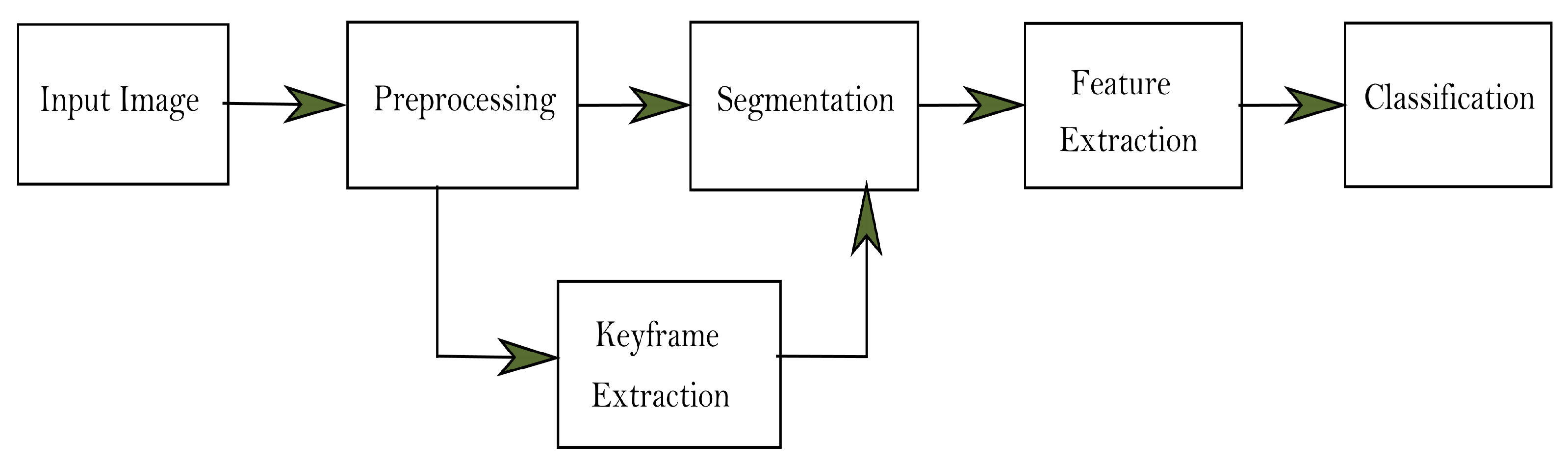
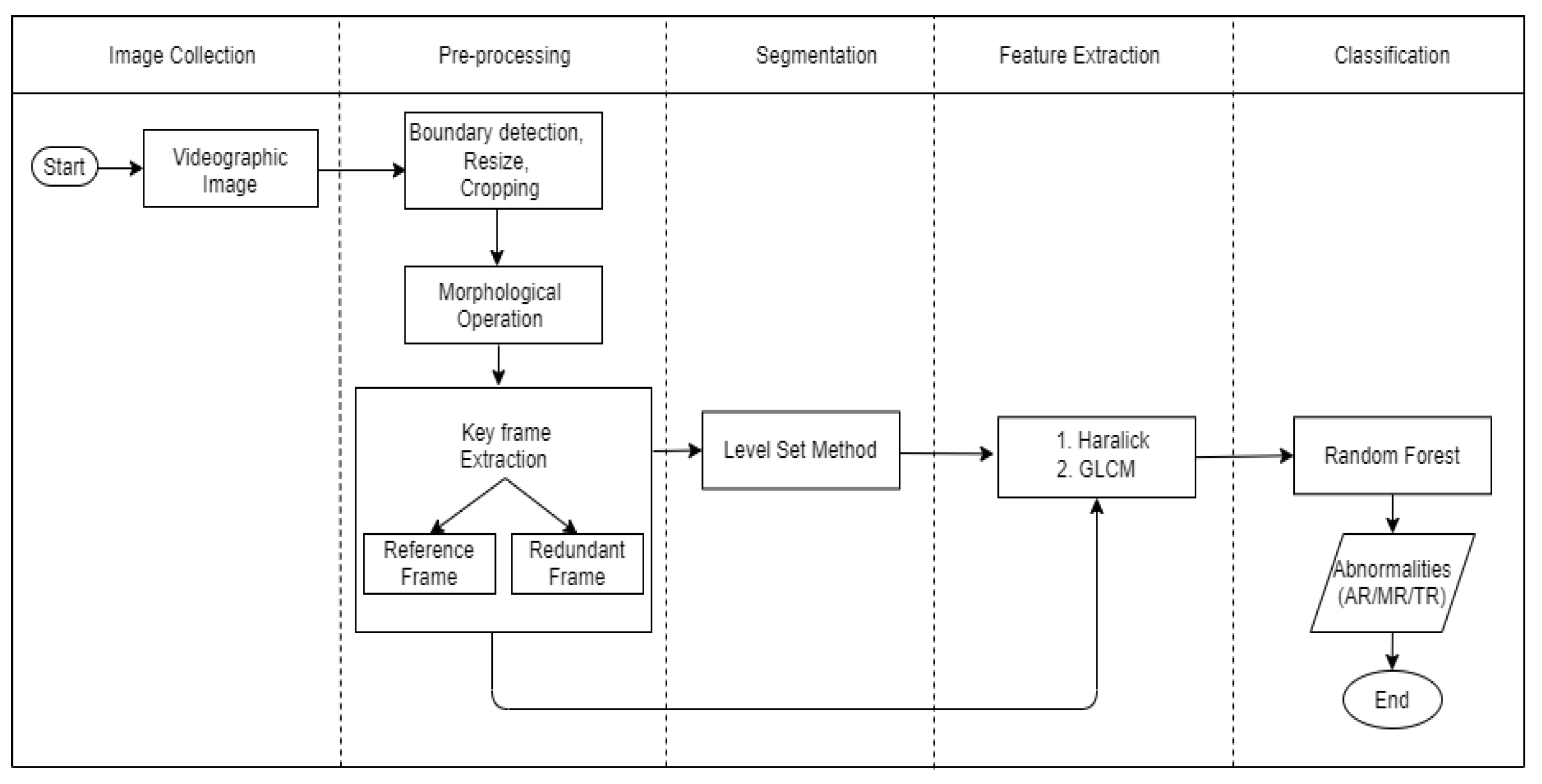
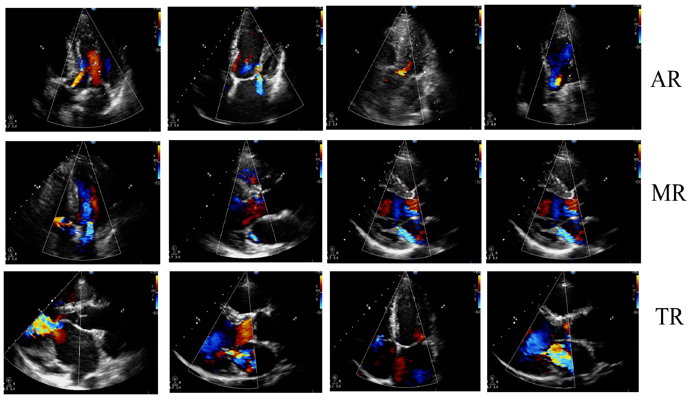
  • An automated system is designed to classify valvular regurgitation using echo with all the steps involved, such as preprocessing, keyframe extraction, segmentation, feature extraction, and classification.
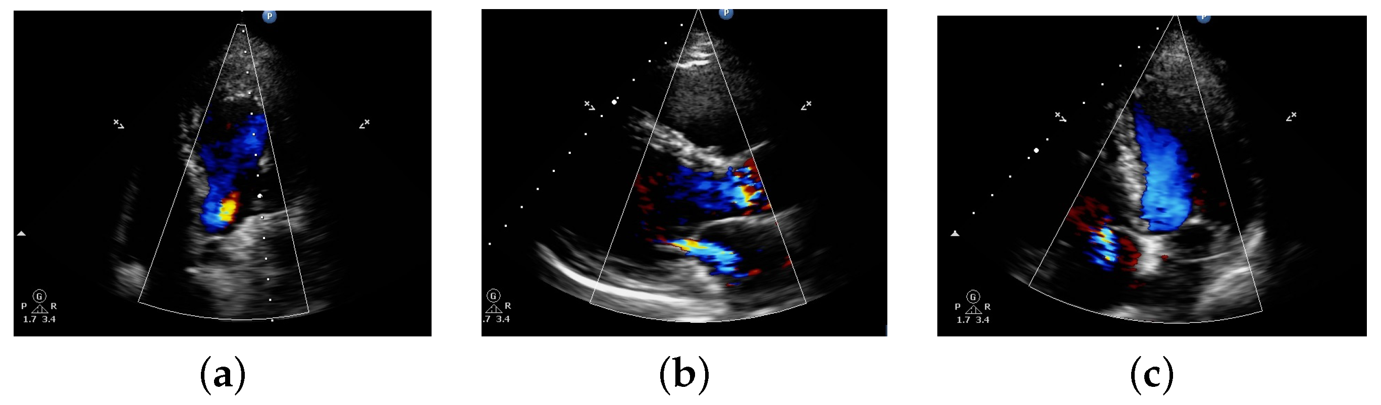
  • In contrast to most of the existing work where authors use image file format, here, we have used videographic images to classify valvular regurgitation.
  • Using videographic images, the number of frames is large, and there may be similar frames. In this work, we have used the keyframe extraction technique, which reduces the number of frames from video and also minimizes redundancy. This is the beginning of the application of keyframe extraction in regurgitation classification. Here, the reference keyframe extraction and redundant frame keyframe extraction techniques have been incorporated.
  • The data used are validated by a cardiologist in the case of classification.
  • The utilization of videographic images, keyframe extraction, and methodologies such as Level set, Haralick features, and GLCM with Random Forest distinguish this research from others.
  • To evaluate the robustness of the model, we have used both segmented images and non-segmented images and evaluate the performance of the model.
  • The results of the proposed method are compared to several existing methodologies, and the results show that our implemented method provides higher performance accuracy than other state-of-art techniques.
The rest of the paper is organized as follows: Works related to regurgitation and heart-related classification are described in Section 2. In Section 3, the methodologies used are explained in brief. Section 4 provides the experimental result, and Section 5 includes the conclusion and future work.

2. Related Works

The heart is a sophisticated structure that requires a trained cardiologist for the proper diagnosis of any abnormalities. Some of the works that deal with the heart perspective related to our work are described below.
Pinjari [8] worked with valvular regurgitation using color Doppler images. Two types of regurgitation were considered, namely MR and AR, whereby the images were first converted into YCbCr space. Two filters were used for noise removal, namely the Wiener filter and Gaussian filter. After filtering using Fuzzy K Means and anisotropic diffusion, segmentation was carried out, and Proximal Isovelocity Surface Area Method (PISA) was used for quantification, which classifies regurgitation into mild mitral regurgitation, moderate aortic regurgitation, and severe aortic regurgitation. Allan et al. [12] used 2D echo and proposed an approach for information extraction in apical view. The procedure takes the information of patients and image for classification into volume and label. For finding intensity and label, Joint Independent Component Analysis (JICA) was used. The approach classified moderate MR with an accuracy of 82%.
Varghese and Jayanthi [24] used an approach for segmentation of echo from videos. A closed curve was used to detect heart boundary and Gaussian Mixture Model (GMM) clustering for segmentation. Balaji et al. [3] worked on view classification using echo. Two features were used namely histogram features and statistical features to classify of four standard views, namely, parasternal short axis (PSAX), parasternal long axis (PLAX), apical two chambers (A2C), and apical four chambers (A4C), was carried out. For 200 images, an accuracy of 87.5% was achieved. Another work by Balaji et al. in [25], similar to that in [3], on view classification was done. Mathematical morphology was used before segmentation using Connected Components Labeling (CCL). Classification of three standard cardiac views, namely parasternal short axis (PSAX), apical two chambers (A2C), and four-chamber (A4C) views, was carried out with an accuracy of 94.56%. Nandagopalan [16] has worked on view classification using a Bayesian classifier. Danilov et al. worked on preprocessing using median filter and Ramponi filter and segmentation using active contours. Supha [26] dealt with the left ventricle (LV) segmentation by detecting LV boundary using fuzzy logic and watershed algorithm along with hidden Markov model-based scheme. Oo et al. [17] used a level set method for LV boundary detection. Mazaheri et al. [18] also worked with LV boundary segmentation and reviewed using level set, active contour, and active shape models. In [27], heart valve disease for aortic stenosis (AS) was assessed. A review on machine learning techniques for heart disease prediction can be seen in [28], and work based on heartbeat counts for the classification of heart diseases could be observed in [29].
In the next section, a discussion on the different existing methods and the proposed approach used for the classification of regurgitation into AR, MR and TR can be observed.

3. Methodology

3.1. Existing Methodologies Used in Proposed Methodology

3.1.1. Gray Level Cooccurrence Matrix (GLCM) and Haralick Texture Features

GLCM is a statistical method of extracting texture features that considers the spatial relationship of pixels in an image. A square matrix of size N × N defines gray level values of pixels at a different position. For the image, I ( i , j ) , the intensity features and texture features that were extracted are Energy, Correlation, Entropy, Contrast, Homogeneity, Mean, Standard Deviation, Root Mean Square (RMS), Skewness, Variance, Smoothness, Kurtosis, shade, prominence and Inverse Difference Normalized, Inverse Difference Moment Normalized (IDM) [30,31]. Haralick texture features are also texture descriptors of an image that specify the spatial relationship among the neighboring pixels in an image [32]. Haralick features are calculated using GLCM and widely used due to their simplicity and perceptive interpretations [33]. The different extracted Haralick features are angular second moment, sum of squares, sum average, sum variance, sum entropy, difference variance, difference entropy, Info measure of correlation 1, and info measure of correlation 2 [34]. Texture features are selected because they provide information about the intensities of an image. Such features partition images into the region of interest and classify them.

3.1.2. Random Forest (RF)

RF is used as it is a stable algorithm having multiple trees and is not biased. It can even take care of missing values in data. RF is a supervised classification technique used in solving classification and regression problems. Two stages are present in the RF algorithm: one is to create the forest, and another is to predict the forest. The RF model calculates a response variable from the randomly created number of decision trees and then puts each feature set to be modeled down each decision tree. The response is then determined by evaluating the responses from all of the trees. At each internal node of the decision tree, entropy is given by the formula in Equation (1) [35].
E n t r o p y = i = 1 n p i X l o g p i
where n = number of classes and p i is the probability of each given classes.

3.1.3. Level Set Methodology (LSM)

It is a method developed in the 1980s that has become popular in imaging processing and computer vision that is used to analyze shapes and surfaces [36,37]. It is used for segmentation where a surface (x) is taken, and a contour is obtained as its output. The front (the point where the surface is at its zero levels) is defined as a zero level set (x = 0). This technique provides accurate numerical as well as adhering to topological changes as well [36]. The intersection of x with the plane creates a contour. For a point, p(a,b) the derived quantity p(t) is its position over time. The evolution of the level set function resembles that of the Hamilton Jacobi equation [38]. It is dependent on partial differential equations, where different parameters are combined to obtain an interface for image segmentation [19]. LSM can be defined in Equations (2)–(4) as follows:
x ( a , b , t ) < 0     i f     ( a , b ) ϕ ¯
x ( a , b , t ) = 0     i f     ( a , b ) τ
x ( a , b , t ) > 0     i f     ( a , b ) ϕ ¯
where ϕ denotes sub region inside τ and ϕ ¯ .

3.2. Proposed Methodology

The major computational steps in the proposed approach are image preprocessing, keyframe extraction, unsupervised segmentation (without ground truth), feature extraction, and classification. The overall flowchart of the algorithm used in the proposed methodology is given in Figure 3, and is explained in subsequent sections.

3.2.1. Image Preprocessing

In this paper, the echo obtained are in Audio Video Interleave (AVI) format which were extracted into frames. To improve feature extraction, the image in the dataset is preprocessed before the extraction of features. The first operation is to normalize the image size, and all the images are resized to 224 × 224 number of pixels. The next step is to convert the RGB image to a grayscale image for better representation of an image. To make the uniform background, a masking operation is performed and finds the region of interest (ROI). Median filtering technique is used to remove the noises and some connected components. Some morphological operations, such as erosion and dilation, are performed to remove the unnecessary pixels, add boundary pixels, and fill small holes in the masked image. After that the following steps are performed:
  • Binarize the image; get the membership of each pixel using label_image.
  • Using regionprops, the area of each object in an image is calculated. It measures image quantities and features.
  • Sort the area and calculate the centroid of the image.
  • Using ismember, the desired image is computed.
  • Store the frames into a folder for each video.

3.2.2. Image Keyframe Extraction

This method overcomes any irregularities in an image boundary and helps reduce and eliminate any artifacts. The obtained frames are then stored in a folder, and keyframe extraction is applied. Two types of frame extraction are used in this paper. Firstly, using reference frame extraction, a static image captured during videographic echo is taken as a reference frame and compared with the frames obtained from the videographic echo. Mathematically, a reference frame R e f i for each patient P i is compared to frames F 1 , F 2 , , F n where n is the number of frames present for each patient i. For this, we have used Euclidean distance to obtain a single or few frames from the videographic echo by eliminating images having a lower similarity index [39]. Similar frames will have a low value, and dissimilar frames will have higher values. The top one or three best values are taken and used for our implementation purpose. This is useful when a reference frame is available to compare but not suitable for videos with no frame as a valid reference frame. Since we have an available reference frame for each video we can compare to every frame of a particular video. Mathematically it can be represented as Equation (5):
d i s t ( i , j ) = j = 1 N i = 1 M ( i j )
where i = Reference frame extracted by an expert, j = A single frame in a video, N = Total number of reference frames and M = Total number of frames.
For video frames having no reference frame, uniform sampling is used where skipping every two frames has been done. This helps in removing redundancy between images. For this, for each frame F in F 1 , F 2 , , F n select F i + 3 where i = 0 upto n. Mathematically for all videos (Vid) it can be written as shown in Equation (6)
i = 1 n V i d i = j = 1 k F j + 3
where j = 1 to k, k = total number of frames present in a video. After keyframe extraction, extraction of features is performed. We have extracted the features from the keyframe in two different forms: one is extraction of features with segmenting the ROI, another one is extraction of features directly from the keyframe.

3.2.3. Image Segmentation

Currently, there are a variety of tools accessible for manually segmenting an image. Such manual work is time-consuming and may potentially result in erroneous results. Here, an unsupervised technique is used for segmentation. Segmentation is carried out using the LSM [17], which is a commonly used deformable model combined with Fuzzy C Means (FCM) [19]. LSM is computationally intensive, but performance-wise has a powerful impact. Segmentation starts with the FCM algorithm, followed by LSM as per [19]. It is used when shapes and contours are involved and can help detect the presence of any regurgitation in an image. Nonetheless, segmentation for nonuniform images is still complex, and research is still being carried out to date.

3.2.4. Feature Extraction Using GLCM Texture Features and Haralick Texture Feature

Different features are extracted from videographic images to describe the image, which is further used for classification. We have used GLCM texture features and Haralick texture feature in our work. These features are selected due to their performance, GLCM is a widely used statistical texture feature and Haralick is an extension to GLCM that develops spatial indices that can be interpreted easily and are correlated. These are inspired by [31,32,40,41]. In this work, a set of 19 statistical texture features are extracted from the segmented and non-segmented images as shown in Table 1 with their mathematical expressions [32,33,34].
Due to the lack of segmentation using features such as GLCM and Haralick features, the segmentation can be reliable. These are robust methods. The features are extracted from the segmented and nonsegmented images, and the values are stored in a comma-separated values (CSV) file.

3.2.5. Classification

Classification is carried out using Random Forest (RF). RF is preferred over other classifiers such as SVM as this paper involves multiclass classification, not binary classification where it is known to perform better [42,43,44]. It also gives us the probability of belonging to the class. It can also handle imbalanced data such as those relied upon in this work. It is robust to outliers [44]. RF classifier works well in small datasets and outperform other ensemble classifier as has the ability to tackle overfitting issues.
The CSV file is read using the readcsv command from the panda library. The data is split into training and testing using the k-fold split command, and then this is fed to a random forest classifier that classifies the testing data into three classes 0, 1, and 2 (AR, MR, and TR, respectively).

4. Experimental Results

4.1. Experimental Setup

For running the program, we have used Python programming. It is implemented using Google Colab, an online, freely-available platform. The libraries and modules used are Matplotlib, Keras, Sklearn and PIL. The detailed specifications of Google Colab hardware used are provided in Appendix A. The different results obtained are given next. The proposed technique follow the same block diagram as shown in Figure 3.

4.2. Dataset

For carrying out the experiment and analysis, data were obtained from Hope Clinic, Shillong. A color Doppler data consisting of five patients’ data in video format was used for each regurgitation. The number of data obtained after reference frame extraction is 170, where for 20% testing data data division is 136 for training and 34 for testing, and the data count obtained after redundant frame extraction is 532, where for 20% testing data data division is 424 for training and 106 for testing. Here, data are divided into 10%, 20%, 30%, 40% and 50% from the total obtained data as testing data. Using k-fold cross-validation, the number of folds is 2, 3, 5, and 8 folds cross-validation. K-fold cross-validation helps to avoid overfitting and resampling of data which aids in assessing the performance of a model. The input images after cropping and resizing can be seen in Figure 4.

4.3. Output of Proposed Methodology

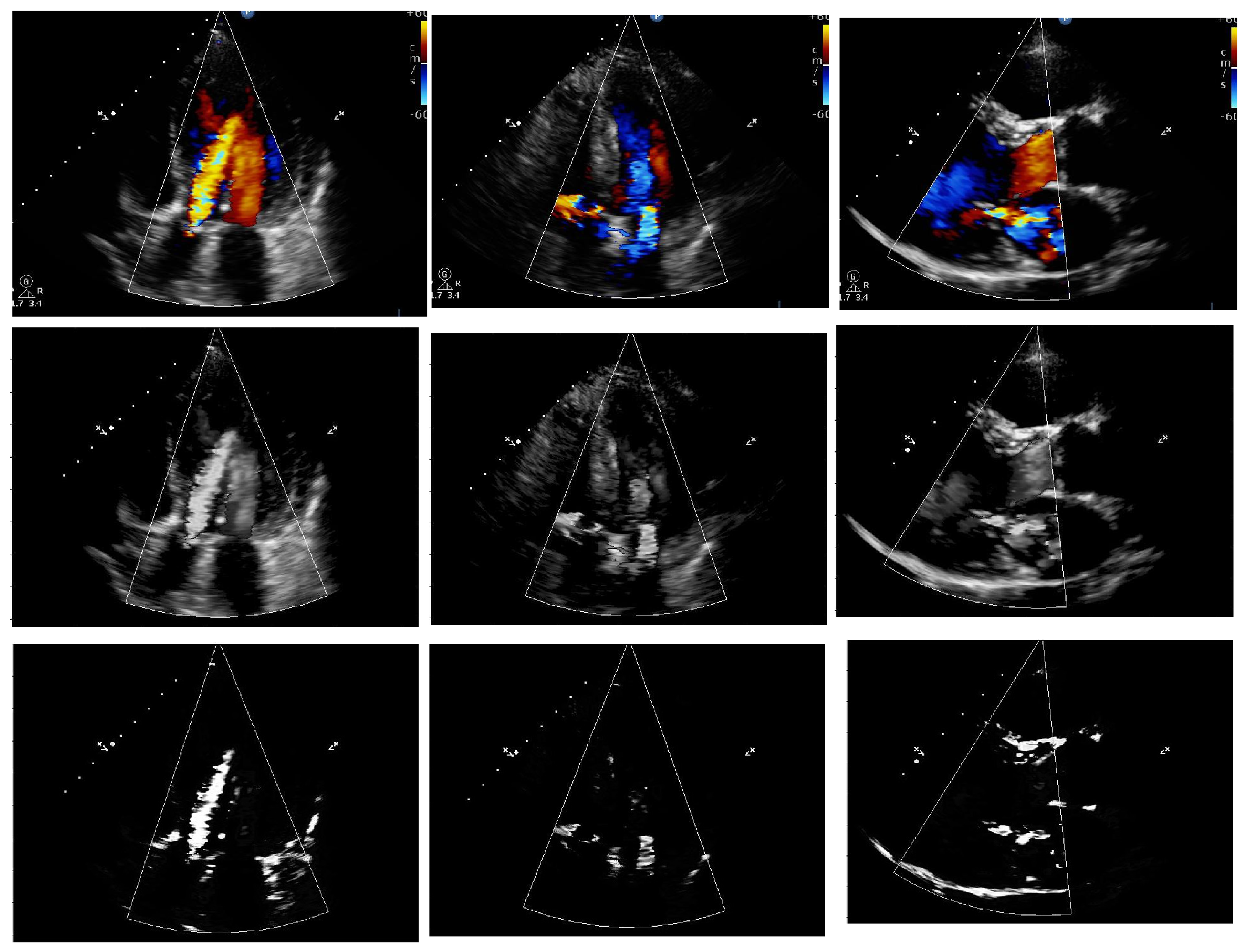
4.3.1. Preprocessing and Segmentation Output

After cropping and resizing, preprocessing is carried out. A preprocessed boundary detection has been applied, and the result can be seen in Figure 5. The figure includes the original images and the preprocessed images. After which segmentation is carried out for both redundant and reference frames. The purpose of this is to test whether segmentation provides a better result or not in later phases of diagnosis, mainly in predicting the presence or absence of any regurgitation in an image.
The output showing segmented images to that of the original images is given in Figure 5. Segmentation is not validated as ground truth is not available for videos. However, the segmented region is carried out for feature extraction, where values of each image are obtained. These values provide the differences and similarities of each frame to one another.

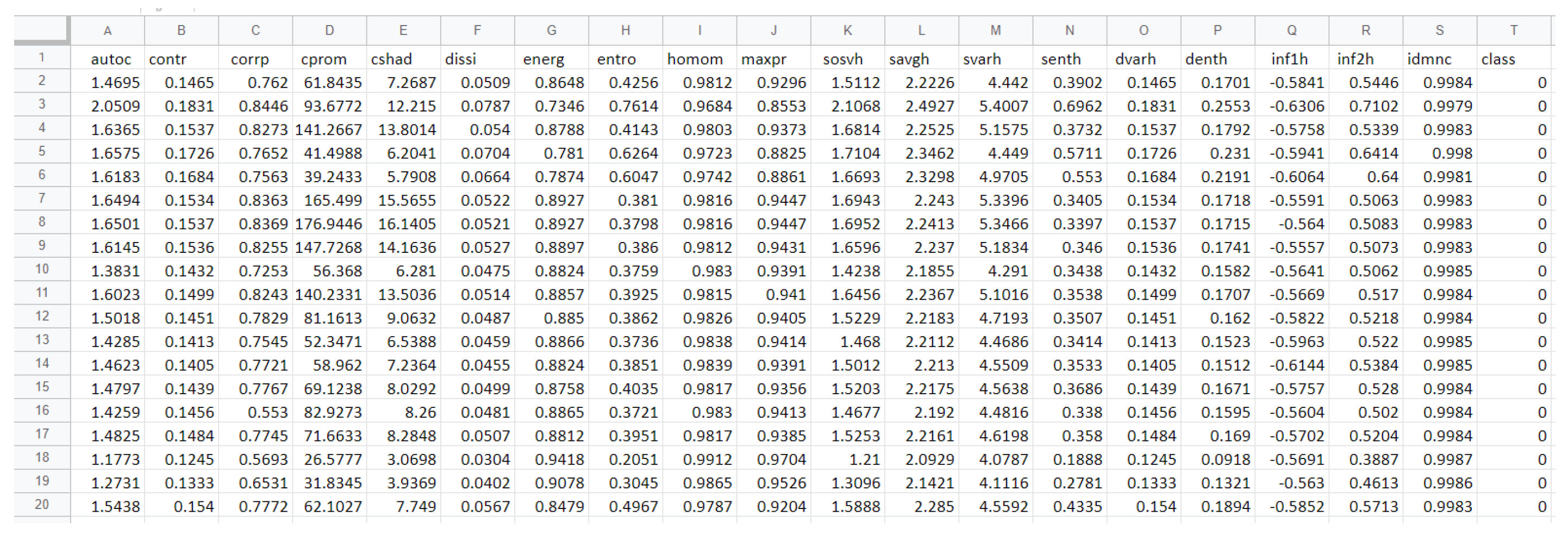
4.3.2. Features Extracted

The different GLCM and Haralick features extracted using Table 1 are stored in a CSV file which look like the image provided in Figure 6. The figure shows obtained features for selected frames. The 19 different features are contrast as c o n t r , dissimilarity as d i s s i , energy as e n e r g , entropy as e n t r o , correlation as c o r r p , homogeneity as h o m o m , variance as s o s v h , autocorrelation as a u t o c , sum average as s a v g h , sum entropy as s e n t h , sum variance as s v a r h , difference entropy as d e n t h , difference variance as d v a r t h , information measure of correlation 1 as i n f o 1 , information measure of correlation 2 as i n f o 2 , cluster prominence as c p r o m , cluster shade as c s h a d , inverse difference normalized as m a x p r and inverse difference moment normalized as i d m n c . With the features, class label is also provided for training phase where 0 is for AR, 1 is for MR and 2 is for TR.

4.3.3. Classification Output

After feature extraction, RF is used to classify the images into three types of regurgitation, namely AR, MR, and TR. Here, two types of classification are carried out which is reference frame classification and redundant frame classification. For each type of classification, two approaches have been used, the segmentation approach and the without segmentation approach. It is crucial to determine whether or not segmentation is an essential factor in classifying regurgitation in the heart. It also gives us a clear idea of validation and analysis of images in the future.
The classification was assessed using four measures based on the confusion matrix. These are Accuracy, Precision, Recall, and F1-score [45]. Classification is implemented using k-fold cross-validation for statistical purposes since data used are not massive.
  • Accuracy: It is the measure of correctly classified images as a percentage. It can be calculated using Equation (7).
    A c c u r a c y = T P + T N T P + F P + T N + F P
  • Precision: It is the fraction of True Positives (TP) and False Positives (FP). Precision can be calculated using Equation (8).
    P r e c i s i o n = T P T P + F P
  • Recall: It represents the fraction of True Positives (TP) and False Negatives (FN). It can be calculated using Equation (9).
    R e c a l l = T P T P + F N
  • F1-score: It is a harmonic mean of precision and recall. It is given by Equation (10).
    F 1 - S c o r e = 2 × Precision × Recall Precision + Recall
The following observations were made based on the output obtained from Table 2, Table 3, Table 4, Table 5, Table 6 and Table 7.
  • Using reference frame extraction, two-fold cross-validation highest accuracy obtained is 85.29% and 91.17% for with segmentation and without segmentation, respectively, and three-, five-, and eight-fold cross-validation highest accuracy is 100% in both cases.
  • Using redundant frame extraction, the best accuracy for two-fold is 87.73% and 98.76%, three-fold is 85.91% and 94.36%, five-fold is 85.71% and 100%, and eight-fold is 84.61% and 100% for with segmentation and without segmentation, respectively.
  • The overall accuracy for two-fold is 76.64% and 83.52%, three-fold is 88.69% and 86.95%, five-fold is 89.22% and 96.46%, and eight-fold is 77.50% and 95% for with segmentation and without segmentation, respectively, in the case of the reference frame, and two-fold is 69.36% and 92.39%, three-fold is 71.26% and 92.71%, five-fold is 63.14% and 96.23%, and eight-fold is 72.30% and 100% for with segmentation and without segmentation respectively in the case of the redundant frame. The overall accuracy of two-, three-, five-, and eight-fold for with and without segmentation for reference frame is 83.56% and 90.48%, respectively. The overall accuracy of two-, three-, five-, and eight-fold for with and without segmentation for reference frame is 69.01% and 95.33%, respectively.
  • Using five folds provided the best result when testing data are divided into 10%, 20%, 30%, 40%and 50%.
  • Based on the output obtained on the accuracy, precision, recall, and F1-score, it can be seen that in most cases, without segmentation gives a better result compared to with segmentation approach. The result that reflects this can be visualized using eight-fold cross-validation, a smaller data distribution using a reference frame.
  • It can be concluded that without using segmentation can also be applied to classify regurgitation in the heart. This might not be the case for all types of diagnosis. It might not be valid for cases of data having ground truth segmentation as well. This can be true for fully unsupervised segmentation techniques and not for supervised or semisupervised segmentation. Using the redundant frame approach provides better accuracy in the case of without segmentation.

4.4. Classification Comparison with Existing Methodologies

To classify AR, MR and TR, the results are compared with SVM and PCA-SVM, which were previously used to classify normal and abnormal images or types of regurgitations. The results of our model is compared with the two methodologies as shown in Table 8. For comparison with other methodologies, taking the average best accuracy of our method, it can be observed that the proposed method is better than the existing method as shown in Table 8. Other parameters are not compared as they are not available in other papers. Moreover, using our data, a comparison is made with PCA + SVM and SVM as a method. Classification is performed using five folds for the existing methodologies, based on the output obtained from Table 6 and Table 7 for the proposed methodology, in which five folds show promising results compared to other folds. The result is provided in Table 9.
The following summary has been observed after implementing the SVM, PCA-SVM, and the proposed approach.
  • From Table 9, it can be observed that our method provides a better result in most cases compared to PCA-SVM and SVM without segmentation and better accuracy to both the methods in the case when using segmentation.
  • In the majority of cases, using 10% testing data provides more promising results than when using 20% or more data. This is mainly due to the data size, which is small in our case.
  • The highest accuracy obtained in SVM, PCA-SVM and the proposed approach is 100% which occurs once in SVM and PCA-SVM and eight times using the proposed approach.
  • Another observation is made where it can be seen that using the redundant frame extraction method, the result is better when using without any segmentation while using reference frame it is better to use with segmentation. This shows that segmentation is more valid and reliable with a known parameter like ground truth than without any ground truth. Furthermore, this is an important aspect of clinical usage.

4.5. Benefits and Limitations of the Proposed Approach

An expert has validated the classification output. Although no deep learning methodologies are used, based on the few datasets using RF as a classifier has overcome that of the SVM classifier, whereas, for binary classification, SVM has been the most used classification technique. RF is used here since it has the capability of distinguishing multiple classes. Overall, the proposed model works as the primary purpose is classification. Segmentation, in this case, is a step that help reduces the size of our data that can be used for feature extraction. Frame extraction, on the other hand, helps reduces slices of data which is crucial as we want only essential slices and not every slice. Our data already consisted of a frame where the exact location of regurgitation appears, but no ground truth was obtained from it.
Data is not large, and no data augmentation is used to test the model’s capability. This deteriorates the performance of a model like deep learning; therefore, a machine learning RF classifier with texture features is used instead of CNN and other relevant models. This work may not be applicable for larger data or any other data as methodologies used are specifically for heart-related field like the LS method. Segmentation output is fully unsupervised, which is not viable for detecting the region of interest. This model is not clinically validated.
Additionally, this effort is technical and not clinical. Clinical usage of a method needs to be precise with efficiency and effectiveness. If more data are fed, the system might not perform well, and we may require a denser model, like deep-learning model that can handle this easily.

5. Conclusions

The use of automated techniques in echo to classify heart regurgitation and its diagnosis has recently emerged in cardiology. In most of the work, researchers identified regurgitation from the image file. In this work, we have designed an automated machine learning-based technique that can be useful in echo regurgitation detection and diagnosis from a video file. Three different types of regurgitation, namely AR, MR, and TR, are considered in this work. One of the advantages of this approach is that the generation of keyframes from the video file which reduces the total number of frames by a large margin. From the results, it is observed that in some folds using segmentation and without segmentation in both reference and redundant frames, the accuracy obtained accuracy is 100% with an overall highest accuracy of 95.33%. In comparison to other techniques proposed by the researchers, as shown in Table 9, the output obtained using our approach is much higher in terms of performance accuracies. Identifying regurgitation from real-time video images in clinics is a crucial future aspect in this area. Though the model gives higher performance accuracies, the dataset used to train and validate the results is small. Using this model in a real-time clinic requires a large number of data to train and validate the model. So, dataset collection based on real-time data is essential in this area.
Using such algorithms will provide a solution to the cardiologist, which will aid in diagnosis and may even assist or replace human efforts in the future. A traditional approach is applied here, which can be studied with additional advanced techniques in the future. Future work also includes the classification of regurgitation severity and early detection of regurgitation, which will reduce the chances of damage to the valves. Also, work with more videographic images and experimentation using deep learning and reinforcement learning models, which are not explored in valvular disease, can be an important aspect of research in this field. These state-of-the-art techniques can tackle and provide higher accuracy, scalability, and efficiency when used correctly.

Author Contributions

Conceptualization, I.W. and A.K.M.; methodology, I.W.; software, I.W.; validation, A.K.M. and G.S.; formal analysis, I.W. and S.M.H.; investigation, I.W.; writing—original draft preparation, I.W. and S.M.H.; writing—review and editing, S.M.H., A.K.M., M.J. and E.J.; supervision, A.K.M., G.S. and M.J.; Funding acquisition, M.J. and Z.L.; project administration, A.K.M., G.S. and Z.L. All authors have read and agreed to the published version of the manuscript.

Funding

The APC was covered by Wroclaw University of Science and Technology K38W05D02 and K43W08ND12.

Informed Consent Statement

Patients’ informed consent was obtained by the clinic.

Data Availability Statement

Limited data are available on request due to the large size of the data.

Acknowledgments

A special appreciation and thanks go to D. S. Sethi, Director of Hope Clinic, Shillong for providing the data and helping in evaluation and identification of the different types of abnormalities.

Conflicts of Interest

The authors declare no conflict of interest.

Appendix A

Specifications of Google Colab.
Filesystem Size Used Avail Use% Mounted on
overlay 108G 38G 71G 35% /
tmpfs 64M 0 64M 0% /dev
shm 5.8G 0 5.8G 0% /dev/shm
/dev/root 2.0G 1.1G 910M 54% /sbin/docker-init
tmpfs 6.4G 32K 6.4G 1% /var/colab
/dev/sda1 55G 38G 17G 70% /etc/hosts
tmpfs 6.4G 0 6.4G 0% /proc/acpi
tmpfs 6.4G 0 6.4G 0% /proc/scsi
tmpfs 6.4G 0 6.4G 0% /sys/firmware
processor : 0
vendor_id : GenuineIntel
cpu family : 6
model : 79
model name : Intel(R) Xeon(R) CPU @ 2.20GHz
stepping : 0
microcode : 0x1
cpu MHz : 2199.998
cache size : 56320 KB
physical id : 0
siblings : 2
core id : 0
cpu cores : 1
apicid : 0
initial apicid : 0
fpu : yes
fpu_exception : yes
cpuid level : 13
wp : yes
flags : flags : fpu vme de pse tsc msr pae mce cx8 apic sep mtrr pge mca cmov pat pse36 clflush mmx fxsr sse sse2 ss ht syscall nx pdpe1gb rdtscp lm constant_tsc rep_good nopl xtopology nonstop_tsc cpuid tsc_known_freq pni pclmulqdq ssse3 fma cx16 pcid sse4_1 sse4_2 x2apic movbe popcnt aes xsave avx f16c rdrand hypervisor lahf_lm abm 3dnowprefetch invpcid_single ssbd ibrs ibpb stibp fsgsbase tsc_adjust bmi1 hle avx2 smep bmi2 erms invpcid rtm rdseed adx smap xsaveopt arat md_clear arch_capabilities
bugs :cpu_meltdown spectre_v1 spectre_v2 spec_store_bypass l1tf mds swapgs taa mmio_stale_data retbleed
bogomips : 4399.99
clflush size : 64
cache_alignment : 64
address sizes : 46 bits physical, 48 bits virtual
power management:
processor : 1
vendor_id : GenuineIntel
cpu family : 6
model : 79
model name : Intel(R) Xeon(R) CPU @ 2.20GHz
stepping : 0
microcode : 0x1
cpu MHz : 2199.998
cache size : 56320 KB
physical id : 0
siblings : 2
core id : 0
cpu cores : 1
apicid : 1
initial apicid : 1
fpu : yes
fpu_exception : yes
cpuid level : 13
wp : yes
flags : fpu vme de pse tsc msr pae mce cx8 apic sep mtrr pge mca cmov pat pse36 clflush mmx fxsr sse sse2 ss ht syscall nx pdpe1gb rdtscp lm constant_tsc rep_good nopl xtopology nonstop_tsc cpuid tsc_known_freq pni pclmulqdq ssse3 fma cx16 pcid sse4_1 sse4_2 x2apic movbe popcnt aes xsave avx f16c rdrand hypervisor lahf_lm abm 3dnowprefetch invpcid_single ssbd ibrs ibpb stibp fsgsbase tsc_adjust bmi1 hle avx2 smep bmi2 erms invpcid rtm rdseed adx smap xsaveopt arat md_clear arch_capabilities
bugs : cpu_meltdown spectre_v1 spectre_v2 spec_store_bypass l1tf mds swapgs taa mmio_stale_data retbleed bogomips : 4399.99
clflush size : 64
cache_alignment : 64
address sizes : 46 bits physical, 48 bits virtual
power management:
MemTotal: 13297228 kB
MemFree: 10934088 kB
MemAvailable: 12479992 kB
Buffers: 58388 kB
Cached: 1655996 kB
SwapCached: 0 kB
Active: 492796 kB
Inactive: 1688232 kB
Active(anon): 984 kB
Inactive(anon): 432992 kB
Active(file): 491812 kB
Inactive(file): 1255240 kB
Unevictable: 0 kB
Mlocked: 0 kB
SwapTotal: 0 kB
SwapFree: 0 kB
Dirty: 196 kB
Writeback: 0 kB
AnonPages: 466716 kB
Mapped: 227304 kB
Shmem: 1272 kB
KReclaimable: 80608 kB
Slab: 109852 kB
SReclaimable: 80608 kB
SUnreclaim: 29244 kB
KernelStack: 4592 kB
PageTables: 8732 kB
NFS_Unstable: 0 kB
Bounce: 0 kB
WritebackTmp: 0 kB
CommitLimit: 6648612 kB
Committed_AS: 2882592 kB
VmallocTotal: 34359738367 kB
VmallocUsed: 9412 kB
VmallocChunk: 0 kB
Percpu: 1416 kB
HardwareCorrupted: 0 kB
AnonHugePages: 0 kB
ShmemHugePages: 0 kB
ShmemPmdMapped: 0 kB
FileHugePages: 0 kB
FilePmdMapped: 0 kB
CmaTotal: 0 kB
CmaFree: 0 kB
HugePages_Total: 0
HugePages_Free: 0
HugePages_Rsvd: 0
HugePages_Surp: 0
Hugepagesize: 2048 kB
Hugetlb: 0 kB
DirectMap4k: 82752 kB
DirectMap2M: 5156864 kB
DirectMap1G: 10485760 kB

References

  1. Mayoclinic: Heart Disease. Available online: https://www.mayoclinic.org/diseases474conditions/heart-disease/diagnosis-treatment/drc-20353124 (accessed on 7 April 2019).
  2. Wahlang, I.; Saha, G.; Maji, A.K. A Study on Abnormalities Detection Techniques from Echocardiogram. In Advances in Electrical and Computer Technologies; Springer: Singapore, 2020; pp. 181–188. [Google Scholar]
  3. Balaji, G.N.; Subashini, T.S.; Chidambaram, N. Automatic classification of cardiac views in echocardiogram using histogram and statistical features. Procedia Comput. Sci. 2015, 46, 1569–1576. [Google Scholar] [CrossRef] [Green Version]
  4. Transthoracic and Transesophogeal Echocardiography (TEE) and Stress-Echo. Available online: https://www.tcavi.com/services/transthoracic-and-transesophogeal-echocardiography-and-stress-echo/ (accessed on 5 March 2020).
  5. Wahlang, I.; Maji, A.K.; Saha, G.; Chakrabarti, P.; Jasinski, M.; Leonowicz, Z.; Jasinska, E. Deep Learning Methods for Classification of Certain Abnormalities in Echocardiography. Electronics 2021, 10, 495. [Google Scholar] [CrossRef]
  6. Lancellotti, P.; Tribouilloy, C.; Hagendorff, A.; Popescu, B.A.; Edvardsen, T.; Pierard, L.A.; Badano, L.; Zamorano, J.L. Recommendations for the echocardiographic assessment of native valvular regurgitation: An executive summary from the European association of cardiovascular imaging. Eur. Heart J. Cardiovasc. Imaging 2013, 14, 611–644. [Google Scholar] [CrossRef] [PubMed] [Green Version]
  7. Varadan, V.K.; Kumar, P.S.; Ramasamy, M. Left lateral decubitus position on patients with atrial fibrillation and congestive heart failure. In Nanosensors, Biosensors, Info-Tech Sensors and 3D Systems 2017; SPIE: London, UK, 2017; Volume 10167, pp. 11–17. [Google Scholar]
  8. Pinjari, A.K. Image Processing Techniques in Regurgitation Analysis; Jawaharlal Nehru Technological University: Anantapuram, India, 2012. [Google Scholar]
  9. Healthy Living. Cardiac Catheterization. Available online: https://www.heart.org/en/health501topics/heart-attack/diagnosing-a-heart-attack/cardiac-catheterization (accessed on 20 April 2019).
  10. Kasthuri, A. Challenges to healthcare in India-The five A’s. Indian J. Community Med. Off. Publ. Indian Assoc. Prev. Soc. Med. 2018, 43, 141. [Google Scholar]
  11. Kumar, R.; Wang, F.; Beymer, D.; Syeda-Mahmood, T. Cardiac disease detection fromechocardiogram using edge filtered scale-invariant motion features. In Proceedings of the IEEE Computer Society Conference on Computer Vision and Pattern Recognition Workshops (CVPRW), San Francisco, CA, USA, 13–18 June 2010; pp. 162–169. [Google Scholar]
  12. Allan, G.; Nouranian, S.; Tsang, T.; Seitel, A.; Mirian, M.; Jue, J.; Hawley, D.; Fleming, S.; Gin, K.; Swift, J.; et al. Simultaneous analysis of 2D echo views for left atrial segmentation and diseasedetection. IEEE Trans. Med. Imaging 2017, 36, 40–50. [Google Scholar] [CrossRef] [PubMed]
  13. Zhang, M.; Tian, L.; Li, C. Key frame extraction based on entropy difference and perceptual hash. In Proceedings of the IEEE International Symposium on Multimedia (ISM), Taichung, Taiwan, 11–13 December 2017; pp. 557–560. [Google Scholar]
  14. Paul, M.K.A.; Kavitha, J.; Jansi Rani, P.A. Key-frame extraction techniques: A review. Recent Patents Comput. Sci. 2018, 11, 3–16. [Google Scholar] [CrossRef] [Green Version]
  15. Ali, I.H.; Al-Fatlawi, T. Key Frame Extraction Methods. Int. J. Pure Appl. Math. 2018, 119, 485–490. [Google Scholar]
  16. Nandagopalan, S. Efficient and Automated Echocardiographic Image Analysis Throughdata Mining Techniques; Amrita Vishwa Vidyapeetham University: Tamil Nadu, India, 2012. [Google Scholar]
  17. Oo, Y.N.; Khaing, A.S. Left ventricle segmentation from heart ECHO images using imageprocessing techniques. Int. J. Sci. Eng. Technol. Res. 2014, 3, 1606–1612. [Google Scholar]
  18. Mazaheri, S.; Wirza, R.; Sulaiman, P.S.; Dimon, M.Z.; Khalid, F.; Tayebi, R.M. Segmentation methods of echocardiography images for left ventricle boundary detection. J. Comput. Sci. 2015, 11, 957–970. [Google Scholar] [CrossRef] [Green Version]
  19. Li, B.N.; Qin, J.; Wang, R.; Wang, M.; Li, X. Selective level set segmentation using fuzzy region competition. IEEE Access 2016, 4, 4777–4788. [Google Scholar] [CrossRef]
  20. Sarica, A.; Cerasa, A.; Quattrone, A. Random forest algorithm for the classification of neuroimaging data in Alzheimer’s disease: A systematic review. Front. Aging Neurosci. 2017, 9, 329. [Google Scholar] [CrossRef] [PubMed] [Green Version]
  21. Kulkarni, V.Y. Effective learning and classification using random forest algorithm. Int. J. Eng. Innov. Technol. 2014, 3, 267–273. [Google Scholar]
  22. Correia, A.H.; Peharz, R.; de Campos, C.P. Joints in Random Forests. Adv. Neural Inf. Process. Syst. 2020, 33, 11404–11415. [Google Scholar]
  23. Kong, Y.; Yu, T. A deep neural network model using random forest to extract feature representation for gene expression data classification. Sci. Rep. 2018, 8, 16477. [Google Scholar] [CrossRef] [Green Version]
  24. Varghese, M.; Jayanthi, K. Contour segmentation of echocardiographic images. In Proceedings of the International Conference on Advanced Communication Control and Computing Technologies (ICACCCT), Ramanathapuram, India, 8–10 May 2014; pp. 1493–1496. [Google Scholar]
  25. Balaji, G.N.; Subashini, T.S.; Suresh, A. An efficient view classification of echocardiogramusing morphological operations. J. Theor. Appl. Inf. Technol. 2014, 67, 732–735. [Google Scholar]
  26. Supha, L.A. Tracking and Quantification of Left Ventricle Borders in Echocardiographic Images with Improved Segmentation Techniques; Anna University: Chennai, India, 2013. [Google Scholar]
  27. Baumgartner, H.; Hung, J.; Bermejo, J.; Chambers, J.B.; Edvardsen, T.; Goldstein, S.; Lancellotti, P.; LeFevre, M.; Miller, J.F.; Otto, C.M. Recommendations on the echocardiographic assessment of aortic valve stenosis: A focused update from the European association of Cardiovascular imaging and the American society of echocardiography. Eur. Heart J. Cardiovasc. Imaging 2016, 18, 254–275. [Google Scholar] [CrossRef]
  28. Aljanabi, M.; Qutqut, H.M.; Hijjawi, W. Machine learning classification techniques for heart disease prediction: A review. Int. J. Eng. Technol. 2018, 7, 373–379. [Google Scholar]
  29. Alarsan, F.I.; Younes, M. Analysis and classification of heart diseases using heartbeat features and machine learning algorithms. J. Big Data 2019, 6, 81. [Google Scholar] [CrossRef] [Green Version]
  30. Wahlang, I.; Sharma, P.; Saha, G.; Maji, A.K. Brain Tumor Classification Techniques using MRI: A Study. Res. J. Pharm. Technol. 2018, 11, 4764–4770. [Google Scholar] [CrossRef]
  31. Suhag, S.; Saini, L.M. Automatic Brain Tumor Detection and Classification using SVM Classifier. Int. J. Adv. Sci. Eng. Technol. 2015, 3, 119–123. [Google Scholar]
  32. Haralick, R.M.; Shanmugam, K.; Dinstein, I.H. Textural features for image classification. IEEE Trans. Syst. Man Cybern. 1973, 6, 610–621. [Google Scholar] [CrossRef] [Green Version]
  33. Löfstedt, T.; Brynolfsson, P.; Asklund, T.; Nyholm, T.; Garpebring, A. Gray-level invariant Haralick texture features. PLoS ONE 2019, 14, e0212110. [Google Scholar] [CrossRef] [PubMed]
  34. Haralick Texture Features. Available online: http://murphylab.web.cmu.edu/publications/boland/boland_node26.html (accessed on 27 April 2019).
  35. Schonlau, M.; Zou, R.Y. The random forest algorithm for statistical learning. Stata J. 2020, 20, 3–29. [Google Scholar] [CrossRef]
  36. Jiang, X.; Zhang, R.; Nie, S. Image segmentation based on level set method. Phys. Procedia 2012, 33, 840–845. [Google Scholar] [CrossRef] [Green Version]
  37. Huang, B.; Pan, Z.; Yang, H.; Bai, L. Variational level set method for image segmentation with simplex constraint of landmarks. Signal Process. Image Commun. 2012, 82, 115745. [Google Scholar] [CrossRef]
  38. Introduction to Level Set. Available online: https://math.berkeley.edu/~sethian/2006/Semiconductors/\protect\discretionary{\char\hyphenchar\font}{}{}ieee_level_set_explain.html (accessed on 27 April 2019).
  39. Euclidean Distance. Available online: https://en.wikipedia.org/wiki/Euclidean_distance (accessed on 2 May 2019).
  40. Brynolfsson, P.; Nilsson, D.; Torheim, T.; Asklund, T.; Karlsson, C.T.; Trygg, J.; Nyholm, T.; Garpebring, A. Haralick texture features from apparent diffusion coefficient (ADC) MRI images depend on imaging and pre-processing parameters. Sci. Rep. 2017, 7, 4041. [Google Scholar] [CrossRef] [Green Version]
  41. Mathworks. Available online: https://www.mathworks.com/matlabcentral/answers/375100-i-want-to-explain-a-detailed-code-glcm-of-my-project-is-detection-on-breast-cancer-and-i-want-to (accessed on 7 April 2019).
  42. Tripathi, A.; Goswami, T.; Trivedi, S.K.; Sharma, R.D. A multi class random forest (MCRF) model for classification of small plant peptides. Int. J. Inf. Manag. Data Insights 2021, 1, 100029. [Google Scholar] [CrossRef]
  43. Rustam, Z.; Sudarsono, E.; Sarwinda, D. Random-forest (RF) and support vector machine (SVM) implementation for analysis of gene expression data in chronic kidney disease (CKD). IOP Conf. Ser. Mater. Sci. Eng. 2019, 546, 052066. [Google Scholar] [CrossRef]
  44. Sleeman IV, W.C.; Krawczyk, B. Multi-class imbalanced big data classification on spark. Knowl.-Based Syst. 2021, 212, 106598. [Google Scholar] [CrossRef]
  45. Vakili, M.; Ghamsari, M.; Rezaei, M. Performance analysis and comparison of machine and deep learning algorithms for IoT data classification. arXiv 2020, arXiv:2001.09636. [Google Scholar]
Figure 1. Diagram showing Doppler echo from the dataset of patients having (a) aortic regurgitation (AR), (b) mitral regurgitation (MR), and (c) tricuspid regurgitation (TR), respectively.
Applsci 12 10461 g001
Figure 2. Flowchart of steps involved in diagnosis of diseases.
Applsci 12 10461 g002
Figure 3. Flowchart of proposed Methodology.
Applsci 12 10461 g003
Figure 4. Input images for AR, MR, and TR.
Applsci 12 10461 g004
Figure 5. The first row shows the input image, second row the preprocessed images and third row the segmented images for AR, MR and TR respectively.
Applsci 12 10461 g005
Figure 6. Features obtained for frames 1–20, as represented in the CSV file.
Applsci 12 10461 g006
Table 1. Features extracted with their mathematical expressions.
Sl. No.Name of FeaturesMathematical Expression
1Contrast f 1 = i = 1 N j = 1 N ( i j ) 2 P i , j
2Dissimilarity f 2 = i = 1 N j = 1 N P i , j | i j |
3Energy f 3 = i j P i , j 2
4Entropy f 4 = i = 1 N j = 1 N P i , j l g P i , j
5Correlation f 5 = i = 1 N ( i μ i ) ( j μ i ) σ i 2 σ j 2
6Homogeneity f 6 = i = 1 N j = 1 N P i , j 1 P i , j 2
7Variance f 7 = i = 1 N P i , j ( 1 μ ) 2 )
8Autocorrelation f 8 = i = 1 N i , j P i , j
9Sum average f 9 = l = 2 2 N l . P x + y l
10Sum entropy f 10 = n = 2 2 N P x + y , n l o g ( P x + y , n )
11Sum variance f 11 = l = 2 2 N ( l f 4 ) 2 P x + y l
12Difference entropy f 12 = l = 0 N 1 P x y l P x + y l
13Difference variance f 13 = l = 0 N 1 l 2 P x + y l
14Information measure of correlation 1 f 14 = H X Y H X Y 1 m a x ( H X , H Y )
15Information measure of correlation 2 f 15 = ( 1 e x p ( 2 ( H X Y 2 H X Y ) ) )
16Cluster Prominence f 16 = i = 1 N j = 1 N ( i + j μ x μ y ) 4 P i , j
17Cluster Shade f 17 = i = 1 N j = 1 N ( i + j μ x μ y ) 3 P i , j
18Inverse Difference Normalized f 18 = i = 1 N j = 1 N P ( i , j ) 1 + k n
19Inverse Difference Moment Normalization f 19 = i = 1 N j = 1 N P ( i , j ) 1 + k 2 n 2
Table 2. Reference frame without segmentation.
No. of
Fold
%PrecisionRecallF1-Score
P0P1P2R0R1R2F0F1F2
2-folds1010078.5710076.9210010086.9587.99100
2010084.6177.7710084.6177.7710084.6177.77
3072.7281.8158.3380.0075.0058.3376.1878.2558.33
4075.0081.8181.6110064.2881.8185.7171.9981.81
5084.6110077.7784.6110077.7784.6110077.77
3-folds1050.0010010010050.0010066.6666.66100
2010066.6687.510080.0077.7710072.7282.34
3075.0060.0010010010071.4285.7175.0083.32
40100100100100100100100100100
5010071.4275.0010071.4275.0010071.4275.00
5-folds1066.6610010010060.0010079.9975.00100
20100100100100100100100100100
30100100100100100100100100100
40100100100100100100100100100
5010085.7110080.0010010088.8892.30100
8-folds10100100010075.00010085.710
20100100100100100100100100100
30100100100100100100100100100
40100100100100100100100100100
5010010050.0010066.6610010079.9966.66
Table 3. Reference frame with segmentation.
No. of
Fold
%PrecisionRecallF1-Score
P0P1P2R0R1R2F0F1F2
2-folds1010028.5790.0055.5510075.0071.4244.4481.81
2083.3369.2377.7783.3310053.8483.3381.8163.62
3081.8172.7275.0060.0010081.8169.2284.2073.68
4075.0072.7210075.0072.7210075.0072.72100
5010058.3310086.6610075.0092.8573.6885.71
3-folds1010050.0072.7272.7210080.0084.2066.6676.18
2088.8850.0010072.7210088.8879.9966.6694.11
30100100100100100100100100100
4010066.6610010010075.0010079.9985.71
5010010087.5088.8810010094.1110093.33
5-folds10100100100100100100100100100
2010066.66055.55100071.4279.990
3010010075.0089.7110010094.5710085.71
4010010060.0066.6610010079.9910075.00
50100100100100100100100100100
8-folds1010033.3310010010033.3310049.9949.99
20100100100100100100100100100
3033.3310050.0010020.0010049.9933.3366.66
4010010075.0066.6610010079.9910085.71
5050.0010010010050.0010066.6666.66100
Table 4. Redundant frame without segmentation.
No. of
Fold
%PrecisionRecallF1-Score
P0P1P2R0R1R2F0F1F2
2-folds1095.2396.7790.9097.5690.9093.7596.3893.7492.30
2095.7499.1710097.8299.5894.4496.7699.3797.14
3088.8871.4293.9386.9586.9583.7887.9078.4288.56
4085.0096.7780.0091.8978.9490.3288.3186.9584.84
5094.5996.6697.5010093.5495.1297.2195.0796.29
3-folds1093.7588.2395.6596.7788.2391.6695.2388.2393.61
2092.5990.0091.6696.1585.7191.6694.3387.8091.66
3091.6690.9088.4684.6190.9095.8387.9990.9091.99
4096.5595.2390.4796.5595.2390.4796.5595.2390.47
5094.4492.8595.2394.4486.6610094.4489.6597.55
5-folds10100100100100100100100100100
2094.1183.3392.3088.8890.9092.3091.4286.9592.30
30100100100100100100100100100
4086.6687.5095.0092.8577.7795.0089.6482.3495.00
50100100100100100100100100100
8-folds10100100100100100100100100100
20100100100100100100100100100
30100100100100100100100100100
40100100100100100100100100100
50100100100100100100100100100
Table 5. Redundant frame with segmentation.
No. of
Fold
%PrecisionRecallF1-Score
P0P1P2R0R1R2F0F1F2
2-folds1080.9564.5148.2779.0750.0073.6879.9956.3358.87
2076.5972.0058.8281.8156.2566.6679.1163.1562.49
3088.8871.4210095.2386.9580.4891.9478.4289.18
4075.0077.4131.4262.5057.1468.7568.1865.7443.12
5081.0855.1742.5062.5059.2561.2970.5857.1350.19
3-folds1087.5081.2586.9587.5068.4210087.5074.2893.01
2048.1445.0058.3354.1639.1358.3350.9741.8658.33
3078.2663.6684.6169.2373.6884.6173.4668.2884.61
4065.5171.4266.6670.3762.5070.0067.8566.6668.28
5083.3371.4266.6685.7152.6382.3584.6060.6073.67
5-folds1077.7766.6666.6677.7761.5372.7277.7763.9969.55
2082.3558.3375.0077.7763.6375.0079.9960.8675.00
3085.7180.0088.8880.0072.7210082.7576.1894.11
4060.0062.5036.8452.9435.7163.6356.2471.6146.66
5062.5069.2384.6183.8352.9484.6171.6159.9984.61
8-folds1066.6671.4240.0060.0050.0066.6663.1558.8249.99
2055.5571.4260.0055.5555.5575.0055.5562.4966.66
3077.7762.5077.7787.5062.5070.0082.3462.5073.68
4081.8190.0080.0090.0081.8180.0085.7085.7080.00
5086.6680.0083.3392.8580.0071.4289.6480.0076.91
Table 6. Performance metrics for 10%, 20%, 30%, 40% and 50% testing data using Reference frame extraction for with and without segmentation for two, three, five, and eight folds.
FoldPerformance
Metrics
With SegmentationWithout Segmentation
10%20%30%40%50%10%20%30%40%50%
2-foldsAccuracy67.6476.4776.4782.3585.2991.1788.2370.5879.4188.23
Precision72.8576.7776.5182.5786.1192.8587.4670.9579.5487.46
Recall76.8579.0580.6082.5787.2292.3087.4571.1182.0387.46
F1-score65.8976.2575.7082.5784.0891.6487.4670.9279.8387.46
3-foldsAccuracy78.2682.6010086.9595.6582.6086.9582.6010082.60
Precision74.2479.6210088.8895.8383.3384.7278.3310082.14
Recall84.2487.2010091.6696.2983.3385.9290.4710082.14
F1-score81.6580.2510088.5695.8177.7785.0281.3410082.14
5-foldsAccuracy10069.2392.3084.6110090.0010010010092.30
Precision10055.5591.6686.6610088.8810010010095.23
Recall10051.8596.5788.8810086.6610010010093.33
F1-score10050.4793.4284.9910084.9910010010093.72
8-foldsAccuracy75.0010050.0087.5075.0087.5010010010087.50
Precision77.7710077.7791.6683.3366.6610010010083.33
Recall77.7710073.3388.8883.3358.3310010010088.88
F1-score66.6610049.9988.5677.7761.9010010010082.21
Table 7. Performance metrics for 10%, 20%, 30%, 40% and 50% testing data using Redundant frame extraction for with and without segmentation for two, three, five, and eight folds.
FoldPerformance
Metrics
With SegmentationWithout Segmentation
10%20%30%40%50%10%20%30%40%50%
2-foldsAccuracy66.6669.8187.7361.3261.3294.3498.7685.8486.7996.26
Precision64.5769.1386.7661.2759.5894.3098.3084.7487.2596.25
Recall67.5868.2487.5562.7961.0194.0797.2885.8987.0596.22
F1-score65.0668.2586.5159.0159.3094.1497.7584.9686.7096.19
3-foldsAccuracy85.9150.7076.0567.6076.0593.0591.5490.2794.3694.36
Precision85.2350.4975.5167.8673.8092.5491.4190.3494.0894.17
Recall85.3050.5475.8467.6273.5692.2291.1790.4494.0893.70
F1-score84.9350.3875.4567.5972.9292.3591.2690.2994.0893.88
5-foldsAccuracy71.4273.1785.7150.0071.4210090.4710090.69100
Precision70.3671.8984.8653.1172.1110089.9110089.72100
Recall70.6772.1384.2450.5973.7910090.6910088.54100
F1-score70.4371.9584.3458.1772.0710090.2210090.22100
8-foldsAccuracy57.6961.5373.0784.6184.61100100100100100
Precision66.0262.3272.6883.9383.33100100100100100
Recall58.8862.0373.3383.9381.42100100100100100
F1-score57.3261.5672.8483.8082.18100100100100100
Table 8. Comparison table for all the methodologies in the classification of heart abnormalities.
AuthorMethodologies UsedTypes of ClassificationType of ImagesAccuracy (%)
Allan [12] (2017)JICA, PCA, SVMTypes of regurgitationStatic82
Kumar [11] (2010)Affine transform, Histogram, Pyramid matching, SVMNormal or abnormal (hypokinesis)Static90.5
ProposedBinarization, Levelset method, Haralick and GLCM, Random ForestTypes of regurgitationVideographic95.33 (Highest obtained accuracy in case of reference frame without segmentation)
Table 9. Performance metrics for 10%, 20%, 30%, 40% and 50% testing data using Reference frame as *Ref and redundant frame as *Red for with and without segmentation.
MethodPerformance
Metrics
With SegmentationWithout Segmentation
10%20%30%40%50%10%20%30%40%50%
SVM (Ref)Accuracy0.880.660.500.510.5010.570.470.420.34
Precision0.900.660.560.520.5610.550.460.440.34
Recall0.900.730.500.480.1710.600.530.530.51
F1-score0.880.630.500.480.4310.560.430.430.73
PCA-SVM (Ref)Accuracy0.700.710.710.640.570.850.570.520.500.51
Precision0.660.690.750.660.580.890.720.510.520.51
Recall0.500.830.810.740.580.890.490.570.640.70
F1-score0.890.630.500.480.430.860.640.520.500.46
SVM (Red)Accuracy0.330.400.420.400.330.900.880.900.900.94
Precision0.330.330.660.580.460.770.790.830.830.92
Recall0.160.160.270.260.250.910.900.920.920.94
F1-score0.220.220.380.370.320.840.840.870.870.93
PCA-SVM (Red)Accuracy0.540.580.470.510.4710.930.950.930.69
Precision0.510.560.470.400.4810.930.940.910.73
Recall0.540.570.470.400.4810.930.960.940.80
F1-score0.530.560.460.500.4810.930.950.920.77
Proposed (Ref)Accuracy10.690.920.8410.901110.92
Precision10.550.910.8610.881110.95
Recall10.510.960.8810.861110.93
F1-score10.500.930.8410.841110.93
Proposed (Red)Accuracy0.710.730.850.500.7110.9010.901
Precision0.700.710.840.530.7210.8910.891
Recall0.700.720.840.500.7310.9010.881
F1-score0.700.710.840.580.7210.9010.901
Publisher’s Note: MDPI stays neutral with regard to jurisdictional claims in published maps and institutional affiliations.

