Improved Deep Recurrent Q-Network of POMDPs for Automated Penetration Testing

Abstract

With the development of technology, people’s daily lives are closely related to networks. The importance of cybersecurity protection draws global attention. Automated penetration testing is the novel method to protect the security of networks, which enhances efficiency and reduces costs compared with traditional manual penetration testing. Previous studies have provided many ways to obtain a better policy for penetration testing paths, but many studies are based on ideal penetration testing scenarios. In order to find potential vulnerabilities from the perspective of hackers in the real world, this paper models the process of black-box penetration testing as a Partially Observed Markov Decision Process (POMDP). In addition, we propose a new algorithm named ${\mathrm{ND}}^3\mathrm{RQN}$, which is applied to the automated black-box penetration testing. In the POMDP model, an agent interacts with a network environment to choose a better policy without insider information about the target network, except for the start points. To handle this problem, we utilize a Long Short-Term Memory (LSTM) structure empowering agent to make decisions based on historical memory. In addition, this paper enhances the current algorithm using the structure of the neural network, the calculation method of the Q-value, and adding noise parameters to the neural network to advance the generalization and efficiency of this algorithm. In the last section, we conduct comparison experiments of the ${\mathrm{ND}}^3\mathrm{RQN}$ algorithm and other recent state-of-the-art (SOTA) algorithms. The experimental results vividly show that this novel algorithm is able to find a greater attack-path strategy for all vulnerable hosts in the automated black-box penetration testing. Additionally, the generalization and robustness of this algorithm are far superior to other SOTA algorithms in different size simulation scenarios based on the CyberBattleSim simulation developed by Microsoft.

1. Introduction

With the development of network technology, people’s daily lives are closely related to networks. A cyber attack is a frequent and severe threat to both individuals and corporations that is caused by many cybersecurity vulnerabilities. The importance of cybersecurity is of global concern. Penetration testing (PT) is an important method for testing cybersecurity that simulates the attacks of hackers to find any potential vulnerabilities in the target networks.

PT refers to the processes, tools, and services designed and implemented to simulate attacks and to find potential vulnerabilities in networks. PT tries to compromise the network of an organization in order to identify the security vulnerabilities. The main objective of PT is to discover potential vulnerabilities that hackers can exploit. In traditional manual PT, professional testers identify the vulnerabilities in the target network based on some prior information about the network such as the topology of network and the software running on the node. The PT path refers to the sequence of PT actions from the start host to the target host that is taken by testers, which enables testers to access the start host and the target host. However, traditional manual PT relies on manual labor. Manual PT requires testers starting over for each new task. The high cost in terms of manpower and resources is an unavoidable disadvantage. Additionally, the existing pool of professional testers is insufficient compared to the large quantity of PT tasks. Automated PT can free up the hands of testers. There is an urgent demand for a reliable and efficient automated PT solution.

Artificial intelligence (AI) is an efficient and credible method. The method used in this paper also combines AI algorithms with traditional methods such as Q-learning. Supervised learning, unsupervised learning, and reinforcement learning (RL) are three different categories of AI methods. Both Supervised Learning and Unsupervised Learning require training on datasets and these methods pay attention to datasets that are extracted and isolated from the environment. However, in the process of PT, penetration testers constantly interact with the network environment and make judgments based on the various network settings of the PT. PT is a sequential decision-making problem. In the process of PT, the agent needs to make decisions based on observations of the environment. At the same time, RL algorithms, which are based on the theory of the Markov Decision Process (MDP), learn what to do to maximize a numerical reward gained in the process of training [1], which is the optimal policy. The agent trained in these RL algorithms is not told which action to take, and through trial and error, must find the maximum reward gained by these actions. The policy is a mapping of the observations of the environment to actions. Typically, the policy is a function approximator, such as a deep neural network. RL does not need static data and only focuses on the interaction with the environment. This characteristic fits well with the automated PT problem.

At present, RL algorithms are used in the field of PT. Zennaro et al. [2] applied Q-learning in a cybersecurity capture-the-flag competition and this application for verified RL algorithms can be used in a straightforward PT scenario. Focusing on the area of SQL injection assaults, Erdodi et al. [3] employed Q-learning to resolve the SQL injection attack planning problem and first portrayed the SQL injection problem as an RL problem.

The study of PT paths is one of the key problems in PT, which requires reducing the probability of detection by defense mechanisms. One autonomous security analysis and PT framework ASAP uses the Deep Q-Network (DQN) algorithm to identify the PT paths provided by Chowdhary et al. [4]. In order to find the PT paths in a variety of situations with varied sizes, Schwartz [5] developed the network simulation tool NASim and applied the improved DQN algorithm. Zhou et al. proposed the enhanced DQN algorithm named NDD-DQN [6] and another algorithm named Improved DQN [7] to identify PT paths. NDD-DQN solves the large action space problem and the sparse reward problem. Improved DQN has greater applicability to large-scale network scenarios and quicker convergence than other state-of-the-art (SOTA) algorithms. The performance of the above improved DQN algorithms, NDD-DQN and Improved DQN, is better than traditional algorithms at convergence speed, robustness, and scalability in a large-scale network setting. In order to solve the high costs of experts and high-dimensional discrete state spaces, Jinyin Chen et al. [8] used the knowledge of experts to pre-train RL and used the discriminator of GAIL for training. GAIL-PT has good stability and lower costs and uses less time, but GAIL combined with other complex RL algorithms would still be complex. However, the above-mentioned researches are all based on MDP, whose testers have complete information about the target network configuration such as the software running on the network nodes and the network topology. In addition, the target of cybersecurity testing is to find potential vulnerabilities that can be exploited by attackers rather than just a path.

Black-box PT, one of the most important types of PT, can provide testers with simulated hackers to interact with environments for testing the security of target networks because testers are not given any inside information, except for the entrance point. Thus, testers require a large amount of specialized knowledge. At the beginning of a black-box PT, testers can only obtain the target network’s entrance information. For penetration testers, the rarely observable information poses a big challenge because it can activate protection mechanisms and even result in failures when the wrong choices are made. Thus, for modeling the black-box PT, the Partially Observed Markov Decision Process (POMDP) can effectively describe the uncertainty of the observations in the target network of the testers. In comparison with the MDP model, the POMDP model adds three additional variables to define the environment from the view of testers. Observation $\mathcal{O}$ stands for testers’ current observable information and provides a partial description of the current state of the global environment. Testers might see the same $\mathcal{O}$ in a different state, which would make it difficult for testers to make decisions. Therefore, the POMDP environment does not suit the MDP algorithms. Furthermore, the experimental findings in Section 3 demonstrate that current MDP algorithms cannot be applied to the larger and more complicated network scenarios of the POMDP model. Zhou et al. [9] recently proposed a path discovery algorithm NIG-AP based on network information gain that uses network information to obtain incentives and direct the agent to take the best action in the POMDP environment. NIG-AP integrates information entropy into the design of the reward values but focuses only on finding a PT path.

The objective of this paper is to find all the potential vulnerabilities in automated black-box PT. In this paper, we first model the process of black-box PT as a POMDP model. Then, we propose a novel algorithm ${\mathrm{ND}}^3\mathrm{RQN}$, which enhances the current traditional DQN algorithms to apply to this new environment. For dealing with a decision problem, we combine Long Short-Term Memory (LSTM) with the DQN in order to deal with the question of the same observation under different states. The structure of LSTM empowers the agent to remember the history, and the agent could distinguish the same observation based on different historical actions. In addition, the enhanced algorithm improves the exploration’s efficiency by the structure of the neural network, which improves the exploration efficiency with decoupling. We change the Q-value calculation method, which decouples the action selection method from the target Q-value generation to solve overestimation problems. Finally, we add noise factors to the neural network parameters, adding randomness to promote the range of exploration of the agent.

The rest of this paper is organized as follows. In Section 2, we introduce the preliminary knowledge of modeling PT using POMDP. In Section 3, we describe the enhanced method of the new RL algorithm. In Section 4, we build four scenarios of different sizes and show the experimental results from the perspective of the mean episode rewards, mean episode steps, and number of detected nodes. Finally, in Section 5, we write a summary of the experimental findings and present the future work.

2. Preliminary

2.1. Penetration Testing

Penetration testing (PT) is a cybersecurity analysis method that is used to check the effectiveness of the defensive strategies set by security workers. Although intrusive by nature, PT is harmlessly bound by a contract, whose target is to find all potential vulnerabilities, rather than exploit the vulnerabilities to cause illegal damage. The testers’ actions in PT are authorized. The steps in the PT process are: prepare, analyze, document, and improve [10]. During the first step, fundamental network-related data are provided to the testers. The amount of information acquired varies depending on the classification of the PT, which is described in the paragraph that follows. In the second step, the tester analyzes the data acquired in the previous step to identify the vulnerable nodes in the target network. The analysis step heavily relies on the tester’s knowledge. To alert developers to the target network vulnerabilities and how to remedy them, the tester documents the PT process. Excellent testers document the vulnerabilities found in this process from two perspectives: the simplicity and potential for exploits, and the complexity and expense of improvements.

The classification of PT is shown in

Table 1. The Classification of Penetration Testing.

Type	Prerequistes	Advantages	Disadvantages
White-box	Testers thoroughly comprehend the target networks’ logical structures.	This method saves time and complete testing can be achieved.	Considered the slowest type of PT.
Black-box	The structures and configurations of target networks are fully unknown to testers, except for the entry points.	This method can simulate a real attack to find unexpected results and is easily understood.	Impossible to perform a complete test.

. This classification is based on how much information a penetration tester can gather beforehand without personally probing the system. As Table 1 shows, PT is divided into black-box PT and white-box PT. White and black represent the degree of visibility of the structure and configuration of the target network. White means visible and black means invisible. In the process of white-box PT, the testers discover potential vulnerabilities based on the pre-known configuration of the target network such as the open ports and running services. In black-box PT, which is based on testers’ professional knowledge and experience, testers probe the information and analyze the target network without any initial internal network information.

2.2. POMDP

The Markov Decision Process (MDP) is a general framework for modeling sequential decision-making problems and is the theoretical basis of reinforcement learning. In the MDP, the transition of an environment’s state is determined by the current state. However, in the real world, environments rarely match the characteristics of MDPs. The Partially Observed Markov Decision Process (POMDP) is a more suitable framework for describing transitions in a real environment. Previously, POMDPs were suggested as a model for PT [11].

POMDPs are usually defined by a tuple $<\mathcal{S},\mathcal{A},\mathcal{O},\mathcal{T},\mathcal{R},\Omega ,b_0>$. We combine PT scenarios to explain their specific meaning. The meaning of $\mathcal{S}$, $\mathcal{A}$, $\mathcal{T}$, and $\mathcal{R}$ are the same as in MDPs. State space $\mathcal{S}$ describes the information about the environment such as the detected host, exploitable vulnerabilities, and so on. Action space $\mathcal{A}$ means that the agent possessed the ability to solve the target tasks such as scanning networks, exploiting vulnerabilities, and so on. Transition $\mathcal{T}\left(s_{t+1}\right|a_t,s_t)$, the probability of the environment’s state transformation, describes how the state of environment changes once the agent has finished its action $a_t$. Reward $\mathcal{R}(a_t,s_t)$ means the value of the results in which the agent interacts with the environment. The agent obtains reward r after finishing action $a_t$ at state $s_t$. In the process of PT, different nodes have different values. For example, the server containing the database is sensitive and the value of this server is certainly high. If the action fails to succeed, the agent would receive a negative reward.

In addition, $\mathcal{O}$, $\Omega$, and $b_0$ are unique to POMDPs. Observation $\mathcal{O}$ is the discrete set of environment observations from the perspective of the agent, and the observation only describes a partial environment, which may be enough to deduce the full information about the environment [12]. The transition of observation $\Omega \left(o_t\right|s_{t+1},a_t)\in [0,1]$ describes the probability corresponding to the current state $s_{t+1}$ and observation $o_t$ after the agent executes $a_t$. Belief $b_0$ means the initial probability distribution of the state [13]. The belief function $b_{t+1}\left(s_{t+1}\right)=Pr\left(s_{t+1}\right|o_t,a_t,b_t)$ is a statistic for the history of actions and observations, which shows the probability distribution of the states [14]. The calculation of belief is as follows:

$$\begin{array}{cc}\hfill b_{t+1}\left(s_{t+1}\right)& =Pr\left(s_{t+1}\right|o_t,a_t,b_t)\hfill \\ \hfill & =\frac{Pr\left(o_t\right|s_{t+1},a_t,b_t)Pr\left(s_{t+1}\right|a_t,b_t)}{Pr\left(o_t\right|a_t,b_t)}\hfill \\ \hfill & =\frac{\Omega (s_{t+1},a_t,o_t){\sum }_{s\in S}^{}Pr\left(s_{t+1}\right|a_t,b_t,s_t)Pr\left(s_t\right|a_t,b_t)}{Pr\left(o_t\right|a_t,b_t)}\hfill \\ \hfill & =\frac{\Omega (s_{t+1},a_t,o_t){\sum }_{s\in S}^{}T\left(s_{t+1}\right|a_t,s_t)b\left(s_t\right)}{Pr\left(o_t\right|a_t,b_t)},\hfill \end{array}$$

(1)

in which state s, observation o, and action a are all the history of the agent in the same training episode.

In the POMDP, the agent can only observe part of the environment (the full state of environment is hidden) and chooses an action based on those observations. The goal of the POMDP tasks is to find a policy that has maximum discount rewards. The optimal policy is given by

$$V_t\left(b\right)=\underset{a\in \mathcal{A}}{max}{Q}_t(b,a),$$

(2)

$$Q_t(b,a)=\mathcal{R}(s,a)+\gamma \sum _{o\in \mathcal{O}}Pr\left(o\right|b,a)V_t\left(b^{o,a}\right),$$

(3)

where the value function $V_t\left(b\right)$ chooses the policy with the highest cumulative Q-value and $Q_t(b,a)$ is the accumulation value of action a when the current belief is b. $\mathcal{A}$ is the set of actions, which is an abstract extract from reality. $\mathcal{R}(b,a)$ is the reward given to the agent when the agent takes action a in belief b. Discount factor $\gamma \in \left[0,1\right]$ is used to charge the importance of current rewards to long-term future rewards. When the value of $\gamma$ is 0 or the smallest designed value, the agent only focuses on the current rewards and could fall into a locally optimal solution. When the value of $\gamma$ is 1 or the largest designed value, the agent focuses on the future rewards. In addition, ${\sum }_{o\in \mathcal{O}}Pr\left(o\right|b,a)V_t\left(b^{o,a}\right)$ means the accumulation of the discount historical reward values. $\mathcal{O}$ is the set of observation from the perspective of the agent. The probability of observation $Pr\left(o\right|b,a)$ means the observation from the view of the agent after taking action a in belief b.

2.3. Reinforcement Learning

Reinforcement learning (RL) is different to supervised learning and unsupervised learning, the target of which is not to characterize a learning method but to characterize a learning problem. RL focuses on using the agent interacting with the environment to find a policy that has a maximum reward based on the abstract environment and target. The core idea of RL is to learn what to do—mapping current environment states to actions—so as to maximize a numerical reward [15].

RL is used to solve sequential decision-making problems after modeling problems using the MDP. In abstract environments, the agent simulating human action in reality continuously interacts with the environment via states, actions, and rewards, as shown in Figure 1, and RL normally stores $(s_t,a_t,s_{t+1},r_t)$ as an episode. In Figure 1, the agent interacts with the environment whose actions are chosen from the action list pulled by the RL algorithm’s demand for the maximum Q value. After taking the action, the environment gives rewards to the agent and the state of the environment changes, which is decided by this action. The list of actions makes up the policy of this training episode. Through trial and error, the target of the agent is to find an optimal policy that has the maximum cumulative Q value or average rewards per episode.

The traditional RL algorithms, such as Q-table and Q-learning, cannot deal with high-dimensional problems. In 2013, Deep Mind proposed a deep Q-learning algorithm [16], which is one of the important starting points for DRL, and this innovation makes DRL outperform arcade learning environments, such as the Atari 2600 game.

3. Methodology

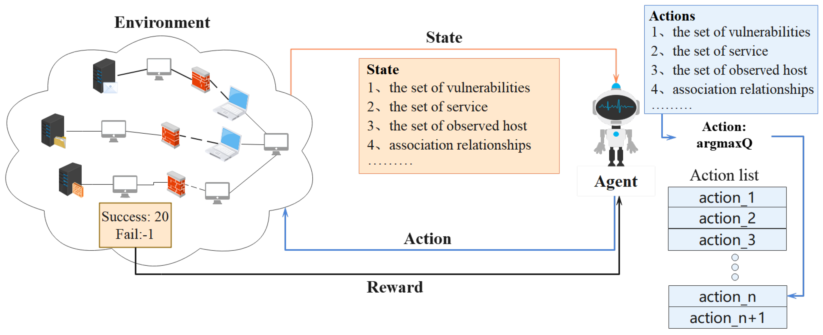
PT is a testing method for assessing network security by simulating authorized hackers’ attacks. When testers test the security of the target networks with the method of black-box PT, they have an incomplete or even complete lack of information about the target networks. In the POMDP model, the agent, which is designed to simulate a human in the real world, also has an incomplete view of the environment. Therefore, in this paper, we use POMDPs to design the process of the automated black-box PT. In POMDPs, the agent cannot decide the next action when observing the same partial information and the MDP algorithms do not work well. However, the previous action in the same process of PT can guide the next action choice. In other words, the action history of an agent within a PT task can assist in decision making. At the same time, LSTM has longer-term memory compared to RNN and better performance in understanding longer semantic sequences. In another words, combing the LSTM and DQN is an improved method of dealing with the decision-making questions in the POMDP [17,18,19].

Furthermore, the POMDP has similar disadvantages to the MDP, and high-quality replay memory is more important in the POMDP, which needs a balance of exploration and exploitation and a better strategic assessment method. Thus, this paper added noise parameters to a neural network to improve the ability of an agent to explore the environment randomly, which could avoid local optimal solutions. The structure of dueling DQN, which is described in detail in the next section, improved the capabilities of the policy evaluation. In addition, this paper delay updated the Q-value function, which reduced the overestimation. To sum up, the new algorithm called N3DRQN integrates all the afore-mentioned components, such as the structure of LSTM, the structure of the Dueling DQN, the Q-value calculation method from the Double DQN, and the noise parameters from Noisy Nets, and is designed to be applied to black-box PT modeled using the POMDP.

The algorithm of ${\mathrm{ND}}^3\mathrm{RQN}$ is described in Algorithm 1, and the training procedure of ${\mathrm{ND}}^3\mathrm{RQN}$ is further explained in the following sections. The meaning of complex signals in following equations and algorithm can be found in

Table A1. The meaning of the symbols in the equations.

Symbol	Mean
($\mu$,$\sigma$)	The learnable parameters in Noisy Nets.
$\epsilon$	The static value.
$\theta$	The noise parameters.
$\zeta$	The linear composition of $\mu$ and $\sigma$.
r	The value of a reward.
$\gamma$	The discount factor.
$\xi$	The set of noise parameters.
$\zeta$	The parameters of the network.

.

Algorithm 1 N3DRQN

Initialize the maximum number of episodes M, the maximum number of steps N Initialize the replay memory D, the set of random variables $\epsilon$ Initialize policy net function $Q^{-}$ with random weights ${\zeta }^{-}$, the target net function Q network with weights $\zeta$, the action selection network $\zeta$″ Initialize the environment $env$ Initialize the target network replacement $N_t$ Initialize the minimum number of episodes $N_{min}$ for episode = 1, M do     Reset the environment state $s_0\sim env$, and observation $o_0\sim \mathcal{O}$     Set $s\leftarrow s_0$, $o\leftarrow o_0$     for step = 1, T do         Sample the noise parameters $\xi \sim \epsilon$         With probability, select action $a_t\leftarrow \underset{b\in \mathcal{A}}{argmaxQ}(o,b,\xi ;{\zeta }^{-})$         execute $a_t$, next state $s^{\prime }=T\left(s^{\prime }\right|s,a_t)$, next observation $o=Z\left(o\right|s^{\prime },a_t)$, reward $r_t=\mathcal{R}(s,a_t)$         Store the transition $(s,a_t,r_t,s^{\prime })$ in D         if $\left|D\right|>N_{min}$ then            Sample a minimum batch of transitions $N_j\leftarrow (s_j,a_j,r_j,s_j^{\prime })$ from D randomly            Sample the noise parameters of the online network $\xi$            Sample the noise parameters of the target network $\xi$′            Sample the action selection network $\xi$″            for j = 1, $|N_j|$ do                if $s_j^{\prime }$ = terminal state then                    $y=r_j$                else                    $a^{*}\left(s\right)\leftarrow \underset{b\in \mathcal{A}}{argmaxQ}(s^{\prime },a,{\xi }^{″};\zeta )$                    $y\leftarrow r_j+\gamma Q(s^{\prime },a^{*},{\xi }^{\prime };{\zeta }^{-})$                end if                Do a gradient with loss ${(y-Q(s^{\prime },a,\xi ;\zeta ))}^2$            end for         end if     end for     if $(episode\%N_t)==0$ then         update the target network $\zeta \leftarrow {\zeta }^{-}$     end if end for

3.1. Extension of DQN

Double DQN. Q-Learning and the DQN both use the maximum action values for selecting the next action, and this value causes a large overestimation. In [20,21], Hado proposed a new algorithm called the Double DQN, which can reduce this overestimation. For a clearer comparison, the core formulas of the two algorithms are listed. Standard Q-learning and DQN algorithms use the equation

$$Y_t^{DQN}=r_t+\gamma \underset{a\in \mathcal{A}}{max}{Q}_t(s_{t+1},a;{\theta }^{-}),$$

(4)

to estimate the value of action $a_t$ in state $s_t$. The part of ${max}_a{Q}_t$ could cause an overestimation because the agent chooses the maximum Q value in the action set $\mathcal{A}$. This part uses the weights of ${\theta }^{-}$ delay updated. Discount parameter $\gamma$ is used to charge the importance of the current rewards. Reward $r_t$ is the reward of the action chosen by the agent in the current state $s_t$.

Compared to a Double DQN, the equations at the same location are as follows:

$$Y_t^{Double}=r_t+\gamma Q_t(s_{t+1},a^{*};{\theta }^{-}),$$

(5)

$$a^{*}\stackrel{def}{=}argma{x}_{a}Q(s_{t+1},a;\theta ),$$

(6)

which are used to select the action. Equation (5) still uses ${\theta }^{-}$ to estimate the value of the greedy policy according to the current value, but a Double DQN selects $a^{*}$ to calculate $Y_t$ that corresponds to the maximum Q value. This tiny change improves the problem of overestimation.

Dueling DQN. A Dueling DQN improves the policy evaluation capabilities by optimizing the structure of a neural network. A Dueling DQN divides the last layer of the neural network into two parts in the Q network. One part is the value function $V(s;\theta ,\beta )$, which is only related to the state s of the agent, and the other part is the advantageous function $A(s,a;\theta ,\alpha )$, which is related to the agent’s state s and action a. Finally, the output of the Q-value function is a linear combination of the value function and the advantageous function

$$Q(s,a;\psi )=V(s;\theta ,\beta )+[A(s,a;\theta ,\alpha )-\frac{1}{\left|A\right|}\sum _{a^{\prime }}A(s,a^{\prime };\theta ,\alpha )],$$

(7)

where $\theta ,\alpha$, and $\beta$, respectively, represent the common parameters of the network, the specific parameters of the advantageous function, and the specific parameters of the value function. The parameter $\psi =\left(\theta ,\alpha ,\beta \right)$ is a combination of the above parameters. The function V is used to evaluate the long-term goals, which is a long-term judgment of the current state s. The function A is the advantageous function, which measures the strengths and weaknesses of the different actions in the current state s.

Noisy Nets. During the process of the agent finding an optimal policy, the importance of balance between exploration and exploitation cannot be ignored. In order to advance the exploration efficiency, Deep Mind [22] proposed Noisy Nets, which are easy to implement and add few computational overheads. The other heuristic exploration methods are limited to small state-action spaces [23,24] compared to Noisy Nets.

Noisy Nets replace the original parameters of the network with noise parameters ${\theta }^{\prime }\stackrel{def}{=}\mu +\sigma \odot \epsilon$, where $(\mu ,\sigma ,\epsilon )$ are random linear parameters and ⊙ represents the dot product. In addition, the equation

$$y\stackrel{def}{=}({\mu }^{\omega }+{\sigma }^{\omega }\odot {\epsilon }^{\omega })x+{\mu }^b+{\sigma }^b\odot {\epsilon }^b,$$

(8)

is used in place of the standard linear equation $y\stackrel{def}{=}\omega x+b$. The random parameters add the stochasticity of neural networks to stimulate the agent to explore the environment. This improvement reduces the probability of the agent falling into local optimum situations. The new loss function of the network is defined as $\overline{L}\left(\zeta \right)\stackrel{def}{=}E\left[L\left(\theta \right)\right]$, which $\zeta \stackrel{def}{=}(\mu ,\sigma )$, $\theta \sim Gaussian(\mu ,\sigma )$.

LSTM. LSTM [25] is one of the most efficient dynamic classifiers and has excellent performance in speech recognition, handwriting recognition, and polyphonic music modeling. LSTM contains three gates (input, forget, output), a block input, a single cell, an output activation function, and peephole connections, and solves the problem of gradient disappearance or gradient explosion in RNNs. The core of LSTM is the use of memory cells to remember long-term historical information and to manage it with a gate mechanism, where the gate structure does not provide information but is only used to limit the amount of information.

3.2. ${\mathrm{ND}}^3\mathrm{RQN}$

In this section, we propose the algorithm ${\mathrm{ND}}^3\mathrm{RQN}$, which was applied to find all the potential vulnerabilities in automated black-box PT. In order to be able to converge, our method used experience replay [26]. This mechanism adds randomness of the data and removes their correlations by randomly sampling from history transitions. In addition, this method set two identical networks to iterative update, policy net and target net [26], to enhance the stability of the algorithm. Target net remains frozen for certain steps; then, the weights of policy net are assigned to the weights of target net.

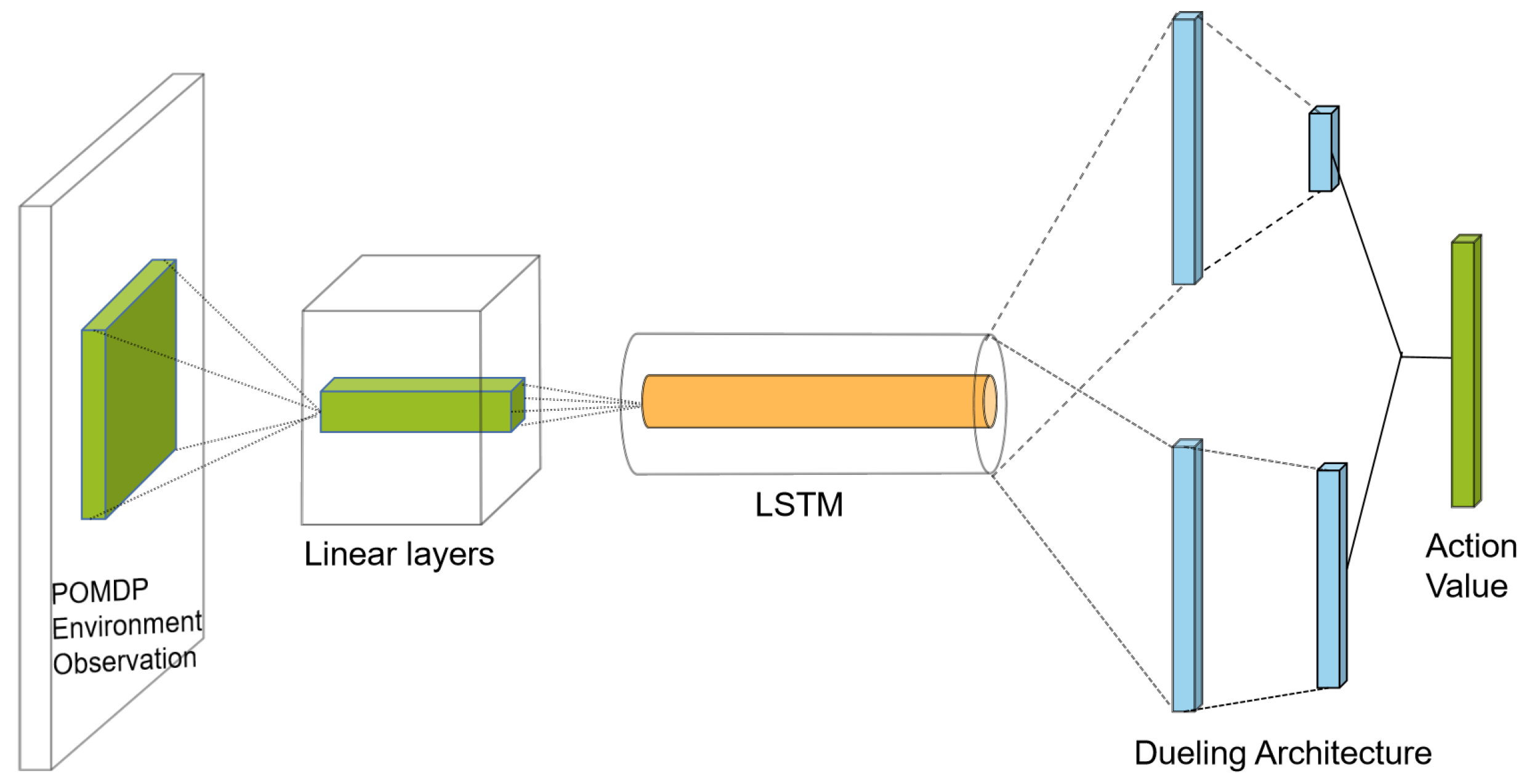
As shown in Figure 2, ${\mathrm{ND}}^3\mathrm{RQN}$ replaced part of the fully connected layers with an LSTM layer, which had the ability for memory. This structure enabled the agent to remember historically chosen actions. In addition, ${\mathrm{ND}}^3\mathrm{RQN}$ combined the structure of the Dueling DQN with the noise parameters for both the Q network and the target network. This change improved the policy evaluation capabilities and used two networks to decouple the action selected from the target Q-value generation to overcome the overestimation problem of the DQN.

The input of ${\mathrm{ND}}^3\mathrm{RQN}$ is a POMDP environment observation vector; the linear layers are fully connected to the input layers and fully connected with each other. The hidden layers consist of the linear layers and the LSTM layer, and the structure of the Dueling DQN added the noise parameters. The output from the structure of the Dueling DQN makes up the two parts that calculate the Q-value. The Q-value is the value of all actions in the next state.

After improving the afore-metioned disadvantages of the DQN, the updated equation of the Q-function is:

$$\begin{array}{c}\hfill y=\left\{\begin{array}{cc}r+\gamma Q(s^{\prime },a^{*},{\xi }^{\prime };{\zeta }^{-}),& otherwise\\ r,& s_t=terminal\end{array}\right.\end{array}$$

(9)

$$a^{*}=\underset{b\in \mathcal{A}}{argmaxQ}(s^{\prime },a,{\xi }^{″};\zeta ),$$

(10)

where $\xi$ is the set of noise parameters, and $\zeta$ is the network parameters. In addition, the overall loss function is defined as

$$\begin{array}{c}\hfill L\left(\zeta \right)={\mathbb{E}}_{(s,a,r,s^{\prime })\sim D}[{(r+\gamma Q(s^{\prime },a^{*},{\xi }^{\prime };{\zeta }^{-})-Q(s^{\prime },a,\xi ;\zeta ))}^2],\end{array}$$

(11)

where $\xi$ belongs to the set of Gaussian noises $\epsilon$ and $a^{*}$ is the optimization from the Double DQN architecture as explained in Equation (10).

$$\begin{array}{c}\hfill L\left(\theta \right)={\mathbb{E}}_{(s,a,r,s^{\prime })\sim D}[{(r+\gamma Q(s^{\prime },a^{*};{\theta }^{\prime -})-Q(s^{\prime },a;{\theta }^{\prime }))}^2],\end{array}$$

(12)

where the noise parameters belongs to the set of Gaussian noises and $a^{*}$ is the optimization from the Double DQN architecture as explained in Equation (10).

Above all, in order for the agent to have memory ability, ${\mathrm{ND}}^3\mathrm{RQN}$ combines the LSTM structures in the neural networks. The structure of the Dueling DQN with the noise parameters creates a balance between exploitation and exploration. In addition, the calculation method of the Q-value is the same as in the Double DQN to prevent overestimation.

4. Experiments

In this section, this paper compares ${\mathrm{ND}}^3\mathrm{RQN}$ with three other algorithms in multiple baseline scenarios, based on the CyberBattleSim simulation developed by Microsoft. Firstly, in order to compare the learning and convergence speed, this paper designed three experimental scenarios to compare the performance of ${\mathrm{ND}}^3\mathrm{RQN}$, RANDOM, DQN, and Improved DQN [7] under the same parameter values. The algorithm Improved DQN is a new algorithm that was proposed last year in the related field. Then, we compared the effectiveness of these four algorithms in a more complex scenario and the goal of these two experiments was to access to all nodes in the network.

4.1. CyberBattleSim and Network Scenario

CyberBattleSim is an open-source project released by Microsoft. This project is based on the OpenAI gym implementation for building highly abstract complex network topology simulation environments. CyberBattleSim provides researchers in related fields with an environment for designing network topologies autonomously.

CyberBattleSim provides three methods for creating a topological environment, as shown in

Table 2. Three methods for creating scenarios provided by CyberBattleSim.

Creation Method	Key Parameters	Means	Network Structure
CyberBattleChain	chainSize	the length of the chain	Chain
CyberBattleRandom	nClients	the number of clients	Random network
CyberBattleToyCtf	nodes and edges	the list of user-defined nodes and edges	User-defined

. Agents can take abstract action extracted from various PT tools in the customized network topology environment. In the initialized environment, the target of the agent is to find the potential vulnerabilities in the target hosts by constantly exploiting vulnerabilities or moving laterally. The success rate of the agent’s action is determined by the experience of experts during the actual PT. The reward function equals the value of the node minus the cost of the action. The more sensitive nodes have a higher value. The cost of the action depends on the qualification of time, money, and complexity. The initial belief is the information about the entrance point in the network. More detailed information can be found on Microsoft’s official website.

The first method, CyberBattleChain, creates a chain-shaped network with a size of input parameters of plus 2, where the start and end nodes are set as fixed. The second method, CyberBattleRandom, uses a function of a randomly generated network in the complex networks to randomly connect generated nodes with different random attributes. The third method, CyberBattleToyCtf, presents a user-defined implementation of the network architecture and nodes.

Based on the above methods, CyberBattleSim creates four typical scenarios for experimentation. The configurations of these scenarios, which each cover a different number of nodes, is shown in

Table 3. The list of network scenarios.

	Nodes	OS	Ports	Services	Remote Vulnerabilities	Local Vulnerabilities
Chain-10	12	4	8	8	2	5
Chain-20	22	4	8	8	2	5
Toyctf	10	3	7	7	8	3
Random	35	4	3	7	1	3

. In order to verify the effectiveness of ${\mathrm{ND}}^3\mathrm{RQN}$ in automated PT, we conducted comparative experiments in the top three different scale scenarios provided by CyberBattleSim: Chain-10, Chain-20, and Toyctf. In addition, we compared the effectiveness of the different algorithms of PT in the scenario Random.

These four basic scenarios all consist of the same elements. Node represents a computer or server in the network, and the information about the OS, Ports, Services, and Firewall Rules is used to describe the node properties. All of these elements are highly abstracted. Vulnerability is another important element, which is described by the type of vulnerability, the precondition of exploiting a vulnerability, the success rate of the exploit, and the cost of the exploit. The full descriptions of these elements are highly abstracted from the real world and details can be found in the open access project CyberBattleSim.

In order to clearly compare,

Table 4. The comparison of states and observations.

State	Observation	Introduction
Discovered node count	none	The number of new node discovered by the agent.
none	Discovered nodes	The list of node information which has been discovered, such as privilege, OS, the configuration of discovered ports and services.
Owned node count	none	The number of new node checked by the agent.
Discovered not owned node	none	The number of new node which is reachable not tested.
Node information	none	The information of each node in the network, if the node tested or not, whether services exist or not.
Discovered services count	List of leaked services	The list of leaked services discovered by the agent.

presents a comparison of the states and observations. State describes the full information about the environment, and observation is the partial information. In this case, state uses three types of information to describe the state of each node in the network, including some nodes not found by the agent. Observation only contains some node information that has been tested by the agent.

4.2. Experimental Results and Discussion

To evaluate the effectiveness of ${\mathrm{ND}}^3\mathrm{RQN}$, we used three metrics to analyze the experimental results separately: mean episode rewards, mean episode steps, and the number of detected nodes. During the training process, the agent takes one action called one step, and all the steps from the initial state to the final goal are called one episode. Mean episode rewards are the mean values of the agent gaining the rewards per episode. Mean episode steps are the mean values of the agent taking the steps per episode. The number of detected nodes means the number of hosts that have vulnerabilities, as detected by the agent.

In this part, this paper used two baseline algorithms, the RANDOM algorithm and DQN algorithm. The RANDOM algorithm selects actions randomly and the DQN [4,27] combines tabular Q-learning and neural networks, which can characterize large-scale state spaces to solve the convergence problem in large-scale state spaces. The Improved DQN [7], which is a recent improvement to the DQN algorithm, was used in the comparison experiments. Through comparing the experimental results obtained in the four scenarios using the above algorithms and metrics, it was found that ${\mathrm{ND}}^3\mathrm{RQN}$’s convergence speed and effectiveness in completing the target task both increased significantly with the complexity of the scenario. The performance of the other algorithms mentioned above was the opposite.

In the first section below, three typical small-scale complex network scenarios are set up: Chain-10, Chain-20, and Toyctf. The results of the experiments are compared using two metrics: mean episode rewards and mean episode steps. These experiments set the achievable goal of gaining access to all the nodes in the network. In the second section, we use a larger scale typical complex network scenario, Random, for comparing these four algorithms’ abilities to gain the target node, which could be transmitted from the metric, that is, the number of detected nodes. In the final section, this paper presents an analysis and conclusion based on the above experiments.

4.2.1. Small Typical Scenarios

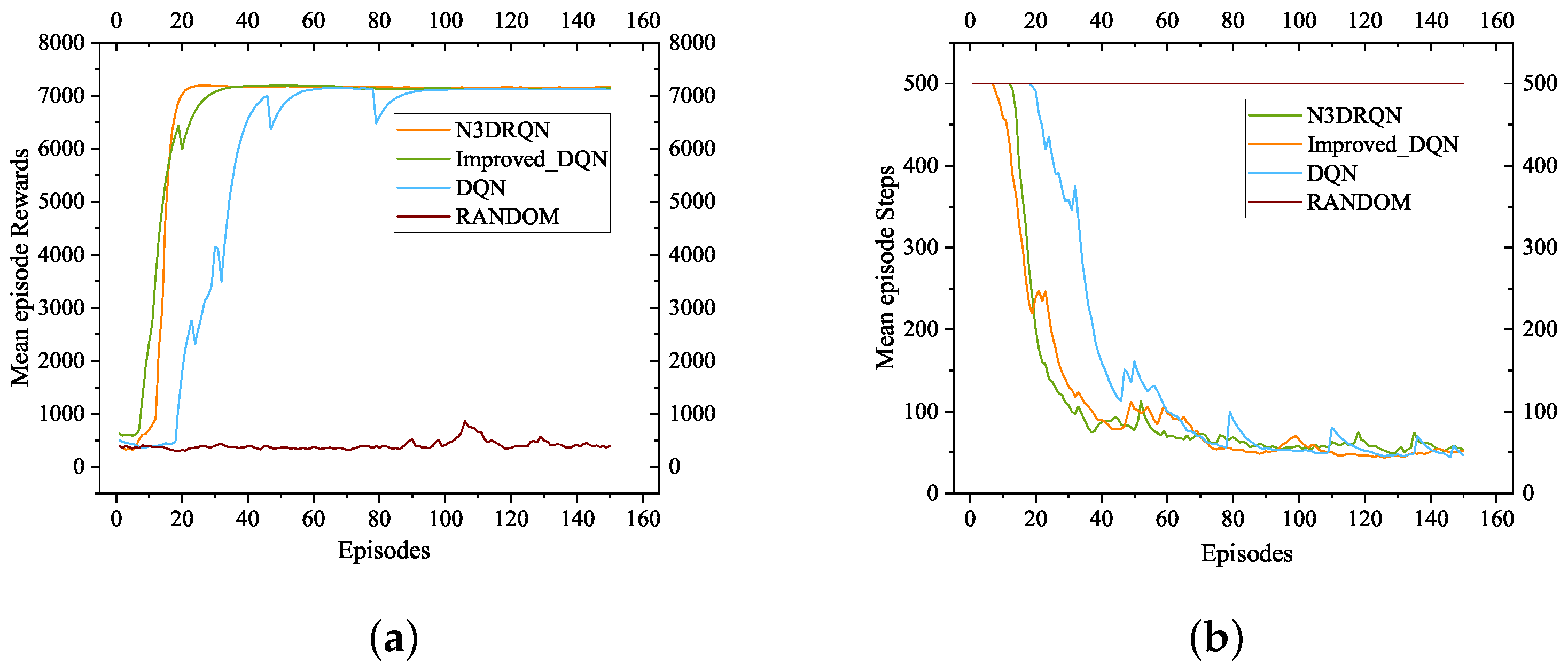
This experiment compares the convergence speed of the RANDOM, DQN, Improved DQN, and ${\mathrm{ND}}^3\mathrm{RQN}$ algorithms in the same scenario with the same parameter values as shown in

Table 5. The list of parameters.

Parameter	Value
learning rate	0.0001
hidden layer size	64
gamma (the discount $\gamma$ in Equation (9))	0.9
iteration counts (total number of step per episode)	500
replay memory size	100,000
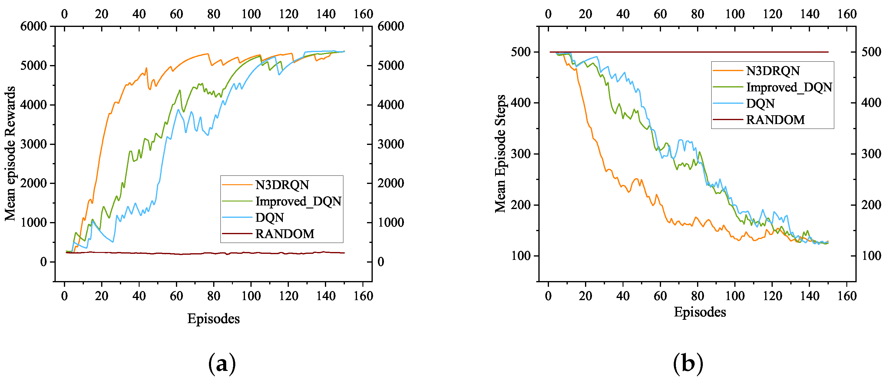
training episode count (total number of episode)	150

. In this part of the experiment, each agent in each algorithm could train 150 episodes, and in each episode, the agent only had 500 times, also known as steps to choose actions. Each episode ended when the number of steps reached 500 or when the experimental target was completed. The target of experiment was to find the optimal policy that could guide the testers to all potential vulnerabilities.

Figure 3a shows the increasing trend in these four methods’ rewards as the number of training times increased in the Chain-10 environment. In addition, Figure 3b shows the decreasing trend in the four algorithms’ step counts per episode as the training times increased in the Chain-10 environment. The horizontal axis in Figure 3 represents the cumulative number of episodes used by the agent to execute the action. The increase in the number of episodes represents the development of the training process. In Figure 3a, the vertical axis represents the mean rewards per episode. In Figure 3b, the vertical axis represents the mean number of steps per episode.

In the Chain-10 environment, the ${\mathrm{ND}}^3\mathrm{RQN}$ and Improved-DQN algorithms started to converge almost simultaneously after around 24 episodes. ${\mathrm{ND}}^3\mathrm{RQN}$ completed the convergence first among these four algorithms. The DQN was a few episodes behind in convergence. The number of steps taken to complete the goal was around 50 except for RANDOM. RANDOM could not converge in the Chain-10 environment.

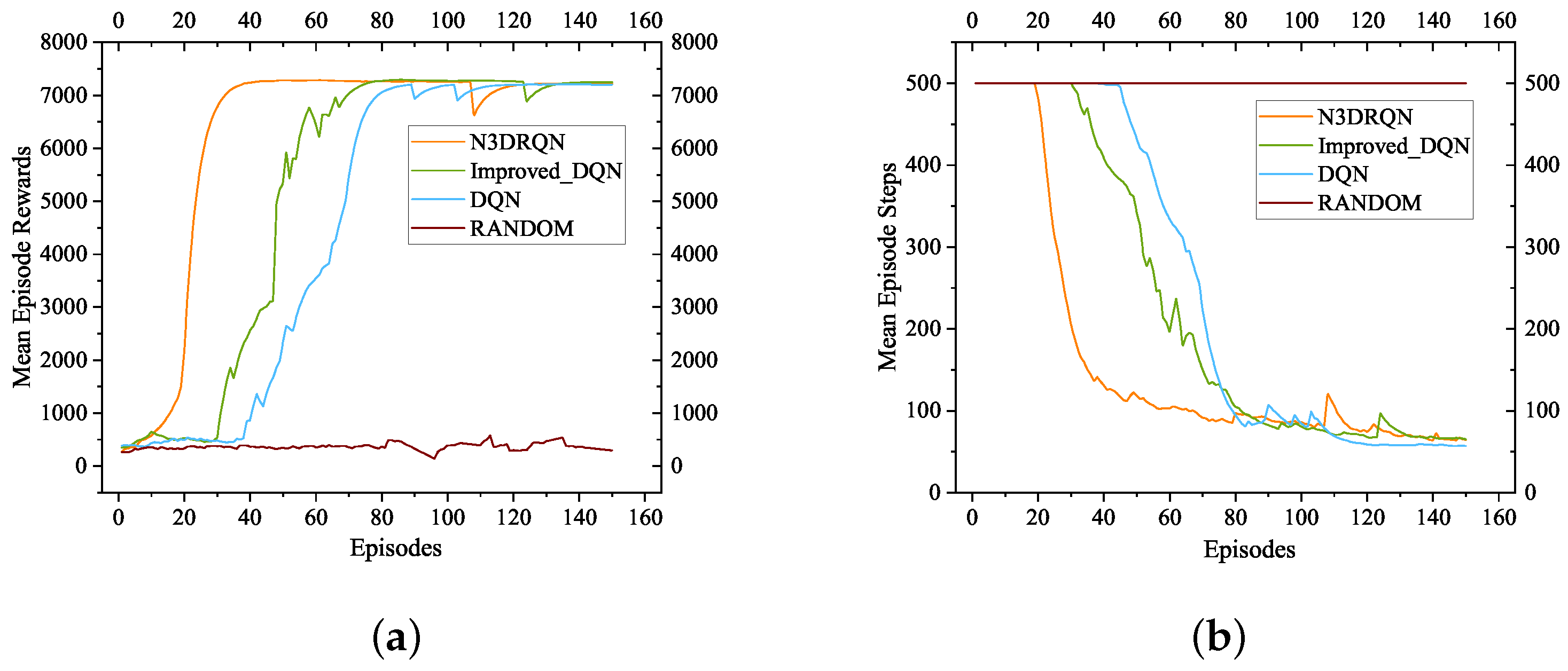
In order to verify the applicability of the improved algorithm ${\mathrm{ND}}^3\mathrm{RQN}$ at larger scales and more complex scenarios, this paper presents another two experiments in this section. The Chain-20 environment had the same structure as the Chain-10 and was compared to 10 more nodes. Additionally, Toyctf was no longer a chained environment, but a more typical structure of a complex network environment in a realistic world. As Figure 4 and Figure 5 show, ${\mathrm{ND}}^3\mathrm{RQN}$ was the first algorithm to converge after about 35 episodes in Chain-20 and about 76 episodes in Toyctf, which means the scaling performance of the improved algorithm was better. At the same time, the convergence order of other methods was the same as the experiment in the Chain-10 environment. RANDOM was still unable to converge. In addition, the least number of steps in the convergence situation showed the same trend, where ${\mathrm{ND}}^3\mathrm{RQN}$ used about 80 steps in Chain-20 and about 130 steps in Toyctf.

Therefore, the efficiency of ${\mathrm{ND}}^3\mathrm{RQN}$ was more evident in the larger or more complex network environments, which means that ${\mathrm{ND}}^3\mathrm{RQN}$ had better robustness in complex and large-scale network environments.

In order to compare the convergence speed clearly,

Table 6. Solved episodes is the minimum episodes for the agent to learn the optimal policy.

Scenario	${\mathbf{ND}}^3\mathbf{RQN}$	Improved-DQN	DQN
Chain-10	24	37	59
Chain-20	35	76	88
Toyctf	76	104	129

presents the number of convergence episodes for the algorithms in the three scenarios, except for RANDOM that never converged. In Table 6, the first column is the name of the scenario and the first line is the name of the algorithm. The other nine numbers are the numbers of convergence episodes for the corresponding algorithm in the corresponding scenario. These numbers are able to show the efficiency of the new algorithm ${\mathrm{ND}}^3\mathrm{RQN}$, which converged faster than the other algorithms. As shown in Table 6, each algorithm was able to find an optimal policy that caused all the potential vulnerabilities in the target network to be compromised while minimizing the number of steps. At the same time, although the environments were constructed with more hosts and more configurations, the performances of all the algorithms dropped.

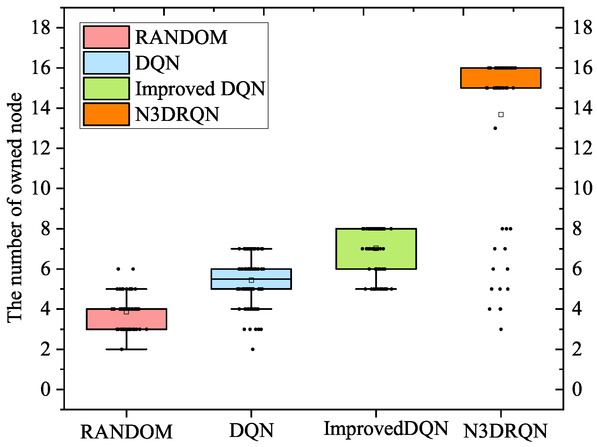
4.2.2. Large Typical Scenarios

In the Random environment, the target of this experimental task was to gain access to all hosts in the current network. We used the metric, number of detected hosts, to analyze the results of the experiment, and we compared the four algorithms’ experimental results, RANDOM, DQN, Improved-DQN, and ${\mathrm{ND}}^3\mathrm{RQN}$. As Figure 6 shows, the horizontal axis represents the algorithms and the vertical axis represents the number of detected nodes. A single point on this box plot represents a result of episodes and the boxes show the areas where the experimental results contain 50% of the experimental results (75%–25%). The lines extending from the boxes are the maximum and minimum values and the other points that are not inside the lines are the outliers.

The order of the results was the same as the above three experiments. ${\mathrm{ND}}^3\mathrm{RQN}$ was far ahead in its ability to perform PT in the POMDP environment, and could obtain a sequence of actions that could access 18 hosts in the Random environment. The other methods performed equally poorly and gained access to up to 8 hosts.

4.2.3. Conclusions

${\mathrm{ND}}^3\mathrm{RQN}$ converged first and had the best results in complicated scenarios according to the results of the four experiments mentioned above. This method was more appropriate for PT in the POMDP environment. The following are the main causes:

1. Our work used POMDP to model the process of automated black-box PT, first based on CyberBattleSim, and improved the algorithm to adapt the agent to the partially observable view. The observation of the agent in the POMDP environment was different from the agent in the MDP environment. The agent chose an action based on the observation, which is always the partial information of the state. Therefore, when the agent was under the same observation but with a different global state, the importance of the historical experience of the agent came to the fore. In other words, the improved ${\mathrm{ND}}^3\mathrm{RQN}$ algorithm incorporated the structure of LSTM to give the agent the ability to remember, and the new ability caused the agent to distinguish the same observation. The agent remembered previously selected action sequences and made a choice based on these past selections.

2. We used three methods for dealing with the balance between exploration and exploitation when training the agent in PT. Thus, the Noisy Nets and the structure of the Dueling DQN were used in ${\mathrm{ND}}^3\mathrm{RQN}$. The neural network imparted a random noise factor via the Noisy Nets, which increased the unpredictability of the parameters. By comparing the short-term and long-term rewards, the agent decided on its current activities, and the rewards pushed it in that direction. In addition to improving the exploration’s efficiency, the issue of overestimating the Q-value was resolved with the introduction of the Double DQN technique.

3. In Section 3, this paper used four experiments to charge the performance of the new ${\mathrm{ND}}^3\mathrm{RQN}$ algorithm. To evaluate how the RL algorithm performance differs with network size, we looked at the scalability of RL. We set four different configuration networks and ran the four mentioned algorithms. As the experimental results showed, all the algorithms were able to find an optimal policy that accessed all the potential vulnerabilities, which minimized the number of steps. However, ${\mathrm{ND}}^3\mathrm{RQN}$ as proposed in this paper converged faster than the other algorithms. In the complex environments, the vulnerability finding efficiency of ${\mathrm{ND}}^3\mathrm{RQN}$ was the best compared to the other three algorithms.

4. Generality is one of advantages of RL. The improved RL algorithms could achievev better performance in a wide range of games [16,26]. Based on this fact, it was feasible to apply RL to different sizes of networks. In addition, current RL algorithms are not able to be directly applied to real network scenarios in automated PT. However, Daniel Arp et al. [28] proposed ten subtle common pitfalls, which led to over-optimistic conclusions when researchers applied machine learning to study and address cybersecurity problems. The limitation of automated PT research field is that current RL algorithms cannot be directly applied to real networks. The reason for this limitation is the high demand for real-time feedback on environmental interactions. The limitation has inspired our team’s future research direction.

5. Conclusions

In this paper, rather than using the MDP to model the PT process, we employed the POMDP model to simulate black-box PT. In the POMDP environment, the original RL method is ineffective. Hence, we mentioned a new method ${\mathrm{ND}}^3\mathrm{RQN}$ that outperformed the previous methods in various areas. Memory and exploration efficiency were enhanced by this method. The convergence performance and efficiency of ${\mathrm{ND}}^3\mathrm{RQN}$ was then evaluated utilizing four different-sized benchmark scenarios provided by CyberBattleSim. These experimental results demonstrated that the improved method ${\mathrm{ND}}^3\mathrm{RQN}$ greatly outperformed the other algorithms in large-scale complex networks. This indicates the advantages of combining a variety of reasonably improved methods.

In future work, we plan to continue to focus on automated PT. On the one hand, we plan to enrich the present agent’s behavioral actions so that they can more closely approximate the behaviors of expert penetration testers. In addition, enriching the current environment to make the simulations more closely reflect real network environments such as adding defense strategies. On the other hand, we plan to research other excellent algorithms such as hierarchical RL or multi-agent RL to improve the performance of the agent. In addition, implementing automated PT in reality is also an important research direction.