Article

TDO-Spider Taylor ChOA: An Optimized Deep-Learning-Based Sentiment Classification and Review Rating Prediction

1
School of Computer Science and Technology, Dalian University of Technology, Ganjingzi District, Dalian 116024, China
2
School of Computer Science and Technology, Dalian Maritime University, No. 1, Linggong Road, Dalian 116026, China
3
Key Laboratory of Intelligent Air Ground Cooperative Control for Universities in Chongqing, College of Automation, Chongqing University of Posts and Telecommunications, No. 2, Chongwen Road, Nan’an District, Chongqing 400065, China
*
Author to whom correspondence should be addressed.
Appl. Sci. 2022, 12(20), 10292; https://doi.org/10.3390/app122010292
Submission received: 18 September 2022 / Revised: 8 October 2022 / Accepted: 10 October 2022 / Published: 13 October 2022
(This article belongs to the Special Issue New Technologies and Applications of Natural Language Processing)

Abstract

:
Modern review websites, namely Yelp and Amazon, permit the users to post online reviews for numerous businesses, services and products. Currently, online reviewing is an imperative task in the manipulation of shopping decisions produced by customers. These reviews afford consumers experience and information regarding the superiority of the product. The prevalent method of strengthening online review evolution is the performance of Sentiment Classification, which is an attractive domain in industrial and academic research. The review helps various domains, and it is problematic to collect interpreted training data. In this paper, an effectual Review Rating Prediction and Sentiment Classification was developed. Here, a Gated Recurrent Unit (GRU) was employed for the Sentiment Classification process, whereas a Hierarchical Attention Network (HAN) was applied for Review Rating Prediction. The significant features, such as statistical, SentiWordNet and classification features, were extracted for the Sentiment Classification and Review Rating Prediction process. Moreover, the GRU was trained by the designed TD-Spider Taylor ChOA approach, and the HAN was trained by the designed Jaya-TDO approach. The experimental results show that the proposed Jaya-TDO technique attained a better performance of 0.9425, 0.9654 and 0.9538, and that TD-Spider Taylor ChOA achieved 0.9524, 0.9698 and 0.9588 in terms of the precision, recall and F-measure.

1. Introduction

Natural Language Processing (NLP) is generally an expansion of linguistics and Artificial Intelligence (AI), which is dedicated to generating computer recognition of the words or statements in human languages. Moreover, NLP is exploited to simplify the work of users and to fulfil the desire for communicating with computers in their natural language. In addition, NLP provides those users who do not have sufficient time to study novel languages or obtain exactness in it, because every user may not be experienced in machine-specific languages. In general, NLP can be separated into two sections, such as natural language creation and natural language understanding, which separates the task into recognizing and formulating the task. The major intent of NLP is to accommodate algorithm specialities to one or more system. Furthermore, the metric of NLP is evaluated on the algorithmic system, which permits combining the language generation and language understanding, and is exploited in multilingual event identification [1]. The approaches employed from the NLP and sentiment analysis areas appear in user expressions and, in turn, assistant emotions with what the user has offered. In addition, cultural standards include various twists to the specific region. For instance, the below declaration can be understood differently. The social media stand affords both prospects and challenges in this region. It provides anonymity to the person writing on the Internet; thereby, the person can express their feeling openly on the positive side. Additionally, the data are collected for specific intervals, which can demonstrate a dynamic that guarantees consistency [2].
Usually, social media is emergent because of the exploitation of innovative services and trends provided by predominant social networking sites. A social media imminent role is specified as an expediter, which improves the analysis and learning of huge data [3]. Moreover, review data dispatched on hospitality and tourism websites, including Yelp, TripAdvisor and Expedia, have attained more academic attention from various practical and theoretical perceptions. Moreover, review data characterize the promising research domain, probably because of their minimal accessibility and cost [4]. Because of the wide range of industrial and academic applications, and also the exponential progression of Web2.0, sentiment analysis is now a hot research area in NLP and data mining. Thus, several techniques and tools proficient in representing the document polarity have been devised recently. In addition, polarity identification is a binary classification task, which is appropriate for various sentiment analysis applications [5,6]. Sentiment Classification [7,8] takes into account mining users’ observations and attitudes, such as negative and positive, from text descriptions formed through user awareness, and is a traditional research topic in the NLP area [9]. Hence, sentiment analysis is also termed as opinion mining, as well as point-of-view analysis, and has been extensively considered in social networks, e-commerce sites and other sections [10,11]. Usually, sentiment analysis is used for the automatic extraction and identification of emotions or sentiments carried by text documents in the practical study region in the text mining field. Sentiment analysis tasks are usually classified into sentence, document and aspect-level analysis with regard to the natural behaviors of text databases [12].
The document-level Sentiment Classification model needs more consideration with regard to structural and relational features at the lower level compared to aspect and sentence-level Sentiment Classification, even though the approach of Sentiment Classification at document-level provides details for sentiment evaluation at other granularities. In general, sentiment analysis is widely classified into binary and ternary Sentiment Classification. The major persistence of categorizing Twitter sentiment is to unavoidably identify sentiment discrepancy in tweets as positive or negative. Usually, Twitter Sentiment Classification observes machine learning schemes in order to formulate a classifier from tweets by means of polarity labels of physically annotated sentiments [3,13]. Commonly, there are three techniques tat are utilized for sentiment analysis, which are the lexicon-based model, such as unsupervised schemes [14], machine learning, such as the supervised method [15], and the hybrid technique, including both unsupervised and supervised schemes. Various approaches by means of deep learning, such as Convolutional Neural Networks (CNN) and Recurrent Neural Networks (RNNs), are more effectual in the text Sentiment Classification process. The integrated machine learning approaches with the deep learning model offered an improved Sentiment Classification performance. Moreover, the Sentiment Classification scheme, depending on the deep learning scheme, utilizes end-to-end patter and also executes classifier and text representation using a neural network [16].
Additionally, preceding approaches for sentiment analysis trained the shallow methods for attaining acceptable polarity classification outcomes. Moreover, these schemes are employed in conventional classification systems, including Support Vector Machines (SVM), Latent Dirichlet Allocation (LDA) and Naïve Bayes, on linguistic features, such as Part-of-Speech (POS) tags, n-grams and lexical features.
The major intention is to devise a Sentiment Classification and Review Rating Prediction technique. Here, review data were taken as the input and pre-processing was performed using a stop word removal and stemming process. Then, most significant features, including SentiWordNet-based statistical features, Term Frequency-Inverse Inverse Document Frequency (TF-IDF)-based features, the number of capitalized words, punctuation marks, numerical words, elongated words, emoticons, hashtags and the number of sentences were mined in the feature extraction stage to enhance classification. Afterwards, the extracted features were passed to the HAN and GRU for Review Rating Predictions and the classification process, respectively. Moreover, the HAN was trained by Jaya TDO algorithm, and the GRU was trained based on TD-Spider Taylor ChOA.
The major contributions of the paper are as follows:
  • Designed TD-Spider Taylor ChoA model for Sentiment Classification: The GRU architecture was applied for performing Sentiment Classification. Additionally, the GRU model was trained by a developed optimization algorithm, named TD-Spider Taylor ChoA, which is newly designed by the combination of ChoA, Taylor series, TDO and SMO algorithms.
  • Developed Jaya TDO-HAN approach for Review Rating Prediction: Here, the HAN model was applied for predicting review ratings from extracted features. Moreover, the HAN model was trained by the proposed Jaya-TDO algorithm. Accordingly, the designed Jaya-TDO was designed by integrating Jaya optimization and the TDO algorithm.
The remainder of the paper is organized as follows: Section 2 describes conventional Sentiment Classification and Review Rating Prediction methods. In Section 3 we briefly introduce the architecture of the proposed framework. The systems’ implementation and evaluation are described in Section 4, and results and discussions are summarized in Section 5. Finally, Section 6 concludes the overall work and future research studies.

2. Related Work

A literature survey of the existing Sentiment Classification and review rate prediction model is explicated in this section. Li L. et al. [17] devised an attention-based Bi-GRU neural network model for Sentiment Classification. Here, the word2vec model was applied for word vector description, and an attention method was exploited for sentiment analysis. The prediction accuracy was high in this method. However, it failed to include fine-grained machine learning schemes for detecting an unpredictable review. Liu, S. and Lee, I. [12] presented sequence encoding with a CNN model for the Sentiment Classification process. The dependency-graph-driven position encoding was improved with weighted sentiment features, and it was combined with feature representation. Moreover, conventional word embedding features were integrated with an encoded sentiment sequence for a revised DCNN for Sentiment Classification. The classification performance was highly enhanced, even though this model failed to embrace large and inclusive data for performing empirical experiments. Alamoudi, E.S. and Alghamdi, N.S. [18] modeled a word embedding and deep learning approach for Sentiment Classification. Here, three various kinds of predictive schemes, deep learning, machine learning and transfer learning, were applied. Yogesh Chandra and Antoreep Jana [7] designed sentiment analysis using machine learning and deep learning. Here, polarity-based sentiment analysis and deep learning models were used to classify the user’s tweets as having positive or negative sentiment. Deep learning models have been implied to classify the tweets. Fatma Jemai et al. [8] devised sentiment analysis using machine learning algorithms. Here, text mining techniques were created to generate and process the variables. In addition, they created a classifier to classify tweets into positive and negative sentiments to evaluate the performance of the model. This method achieved greater precision.
Furthermore, an unsupervised technique was exploited for aspect-level Sentiment Classification. Moreover, it permitted the ability of pre-trained language methods and removed more difficulties linked to supervised learning methods. The computational complexity was lower in this method, even though it failed to resolve mislabeled review issues. Chugh, A. et al. [3] presented a Spider Monkey Crow Optimization Algorithm (SMCA), along with a Deep Recurrent Neural Network (DeepRNN), for Sentiment Classification and information retrieval. Stemming and stop word removal were applied for eradicating undesirable data, and feature extraction was also carried out for the classification process. Fuzzy K-Nearest Neighbor (Fuzzy KNN) was utilized for retrieving data using a distance measure. Feng, S. et al. [19] devised InterSentiment through connecting the model user–product interaction and sentiment methods by means of deep learning. This method learns about high-level depictions by linking review sentiment and the user–product interaction, which was used for rate scoring. The error rate was highly reduced, although it failed to perform other recommendation tasks. Zheng, T. et al. [4] presented a deep learning model for Review Rating Prediction. Here, a biased rating was elucidated and the matching rules were also inclined. Moreover, data pre-processing was carried out and then feature extraction was carried out for review prediction. This approach obtained a better prediction performance, but the user had a limited amount of reviews. Ahmed, B.H. and Ghabayen, A.S. [20] designed a deep learning technique for Review Rating Prediction. This approach mainly comprised two segments, namely the Bi-GRU technique and a deep learning bidirectional gated recurrent unit. Here, the first section contains polarity prediction, and the second phase employed a review rating process from review data. The processing time was lower in this method, although it did not use other languages. Sadiq, S. et al. [21] introduced a deep learning approach for Review Rating Prediction. This approach mainly comprised a review rating and star rating. The polarity of the review was predicted based on sentiment analysis for generating a ground truth. Then, in the second stage, a star rating was predicted from a text setup of the review on the ground truth. The prediction performance was highly improved, even though the effectual datasets were not considered in this method for obtaining a better performance.
The challenges experienced by the existing Sentiment Classification and Review Rating Prediction model are specified as follows:
  • It is essential to detect and understand the user’s feelings in a sensitive complex environment for efficient Sentiment Classification. Moreover, it is not effective to implement semantic classification approaches in the event directly because of the restrictions, such as the standard emotion thesaurus.
  • An attention-based Bi-GRU neural network technique was designed in [12] for Sentiment Classification. However, it failed to utilize a publicity balanced database for the training process, and also did not include a combination of clustering and over sampling methods to generate samples as more balanced.
  • The sequence encoding with the CNN model was designed in [12] for Sentiment Classification, although it did not consider fine-tuned granularity with multi aspects and the attention model to generate adjusted sentiment sequence encoding.
  • Word embedding and deep learning were introduced in [18] for classifying the sentiment, even though it failed to perform word embeddings training on informal dialects to improve the performance.
  • In [3], an SMCA-driven DeepRNN was developed for Sentiment Classification and Review Rating Prediction, but, still, the advanced features, including feature weighting and n-grams, were not considered in this approach for improving the system performance.
The main objective of this research is to design an approach for performing Sentiment Classification and review rating prediction

3. Proposed Method

The block diagram of the proposed Sentiment Classification and Review Rating Prediction using an optimized deep learning model is displayed in Figure 1.
Originally, a review from Facebook was taken as an input and pre-processed based on stop word removal and stemming to remove redundant data. Meanwhile, the significant features were extracted from pre-processed image for effectual classification. Here, the most imperative features, including sentiwordnet features, statistical features, such as standard deviation, mean, variance and classification, and specific features, such as the amount of capitalized words, numerical words, punctuation marks, emoticons, elongated words, Term Frequency-Inverse Document Frequency (TF-IDF) [22], quantity of words in a review, hashtags, number of sentences in a review, average word length and question marks, were extracted from pre-processed data. After that, Sentiment Classification was carried out using a Gated Recurrent Unit (GRU) [23], which was trained based on the proposed Tasmanian Devil Spider Taylor-based Chimp Optimization Algorithm (TD-Spider Taylor ChOA). However, TD-Spider Taylor ChOA was newly developed by assimilating the Tasmanian Devil Optimization (TDO) approach with the Spider-Taylor-based Chimp Optimization Algorithm (Spider Taylor-ChOA). In conclusion, Review Rating Prediction was carried out by Hierarchical Attention Network (HAN) [24], along with the extracted features as input, and it was trained based on proposed Jaya Tasmanian Devil Optimization (Jaya-TDO) algorithm. Here, Jaya-TDO approach was newly formulated by incorporating Jaya algorithm and TDO approach.

3.1. Acquisition of Input Data

Let us consider the review data from a dataset M with v samples, which are illustrated as
M = M 1 , M 2 , , M t , , M b
where M t denotes tth data from a dataset, and b designates the total amount of data.

3.2. Pre-Processing Using Stop Word Removal and Stemming Method

The input review data M t were pre-processed based on stop word removal and stemming, which eliminates the redundant data, thereby increasing image qualit.
(i) Stop word removal: The words, such as articles, pronouns and prepositions, present in a sentence are termed as stop words. In addition, they must be separated before further processing; here, noises that exist in the input data were eliminated by non-information performance words. The separation of stop words helps us to enhance the process and evades more storage space.
(ii) Stemming: This model removed the prefixes and suffixes from input, which reduced the inflected words to their stem. This model was applied to eliminate feature quality in feature space, which improves the clustering performance when the different structures of features are stemmed into a single feature. Moreover, non-meaningful words from language roots were exterminated in the stemming procedure.
The output of pre-processed data was specified as H t and passed to the feature extraction segment.

3.3. Feature Extraction

The most imperative features were extracted from the pre-processed data H t , wherein statistical, sent word net and classification-specific features were extracted for further Review Rating Prediction and sentiment classification.
(i) SentiWordNet features: It helps to cluster the words into various groups of synonyms specified as Synsets. Every Synset is connected with a polarity score, such as positive and negative. The score acclimatizes the rate in 0 and 1, as well as its summation, providing the rate of 1 for all Synset. It is more dependable to decide whether the evaluation is positive or negative by considering the considered score. Moreover, words included in this feature are specified using parts of speech obtained from WordNet, thereby utilizing a program to designate score to every word. The weight tuning of the positive and negative scores is illustrated by
v j ( n ) , v j ( o ) = h y j
where v j ( n ) denotes positive score, v j ( o ) refers to negative score and h symbolizes SentiWordNet. The extracted SentiWordNet feature is denoted as G 1 .
Statistical features: The statistical features, including variance, mean and standard deviation, were extracted from the pre-processed output.
(a) Mean: It was evaluated by means of SentiWordNet: average for all words from the pre-processed review data, and given by
ζ = 1 A g k × n = 1 A g k A g k
where n implies total words, A g k denotes SentiWordNet score of every review and  A g k is total scores created from a word and means that the feature is denoted as s 1 .
(b) Variance: this feature was computed depending on the mean value, which is illustrated by
δ = n = 1 A g k g k ζ A g k
where ζ refers to the mean value and s 2 is specified as the variance.
(c) Standard deviation: this feature was assessed based on the square root of the variance, which indicates the statistic, which gauges a database distribution from the mean rate. The mean difference from every data point was utilized for identifying the standard deviation, and is the same as the square root of variance. The standard deviation is calculated by
λ = 1 Z x = 1 Z f y δ
where Z implies the number of attributes and records in a review data, f y are terms in a given data, δ denotes mean rate and the standard deviation is referred to as s 3 .
The statistical feature is a combination of standard deviation, variance and means feature, which is deliberated as
G 2 = s 1 , s 2 , s 3
Classification-Specific Features: The classification-specific feature comprises punctuation marks, elongated words, hashtags, emoticons, number of sentences in a review, number of words in a review, average word length, question marks, capitalized words, numerical words and TF-IDF, and these are explained below.
(a) Numerical words: They are defined as the total amount of numerical digits and text characters exploited for representing numerals, which is denoted as c 1 .
(b) Punctuation marks: They are represented as an exclamation mark, dot or apostrophe included in review data, and are denoted as c 2 .
c 2 = f = 1 v V l f
where V l f is the total number of punctuations included in the fth review.
(c) Elongated words: They are referred to as elongated words, and are a character repeated more than two times in a review data. They are computed by
c 3 = f = 1 v μ l f
where μ l f denotes total number of elongated words existing in fth review.
(d) Hashtags: They are specified as a consideration of letters, emoticons or numbers termed by the # symbol, and are used for categorizing the contents and generating them as more explorable, and the hashtag feature is specified as c 4 .
(e) Emoticons: They are represented as the short sequence of keyboard letters and symbols, which is denoted as c 5 .
(f) Number of sentences in a review: A sentence is referred to as set of words that makes a statement, expresses a comment and requests questions, wherein total count of sentences is denoted as c 6 .
(g) Number of words in a review: It is referred to as the number of words in a sentence, and is represented as c 7 .
(h) Average word length: It is represented as whole length of text existing in a review document, which is expressed as c 8 .
(i) Question mark: This feature means that the sentence is very likely to be a question, although 25% of questions are short of question mark. Moreover, amount of question marks in a review sentence is extracted, which is specified by c 9 .
(j) TF-IDF: It is a statistical model used to evaluate the important words in a document, where term frequency refers to number of times in which term appears and inverse frequency document frequency specifies the number of documents containing term [22]. It is defined by
c 10 = E log 1 + ς 1 log ς 2
where E refers to the amount of review data, ς 1 is term frequency, ς 2 represents inverse document frequency and TF-IDF feature is c 10 .
Here, the classification of specific feature is denoted as G 3 , which is the combination of above all features in Section 3.3 and is represented as
G 3 = c 1 , c 2 , , c 10
All of the above extracted features were combined to generate a feature vector, which is expressed by
G t = G 1 , G 2 , G 3
where G 1 denotes sentiWord net feature, G 2 represents statistical features and G 3 indicates classification-specific features.

3.4. Sentiment Classification

From the above extracted features, Sentiment Classification was carried out using GRU, and was trained by designed TD-Spider Taylor ChOA in order to improve the classification performance.

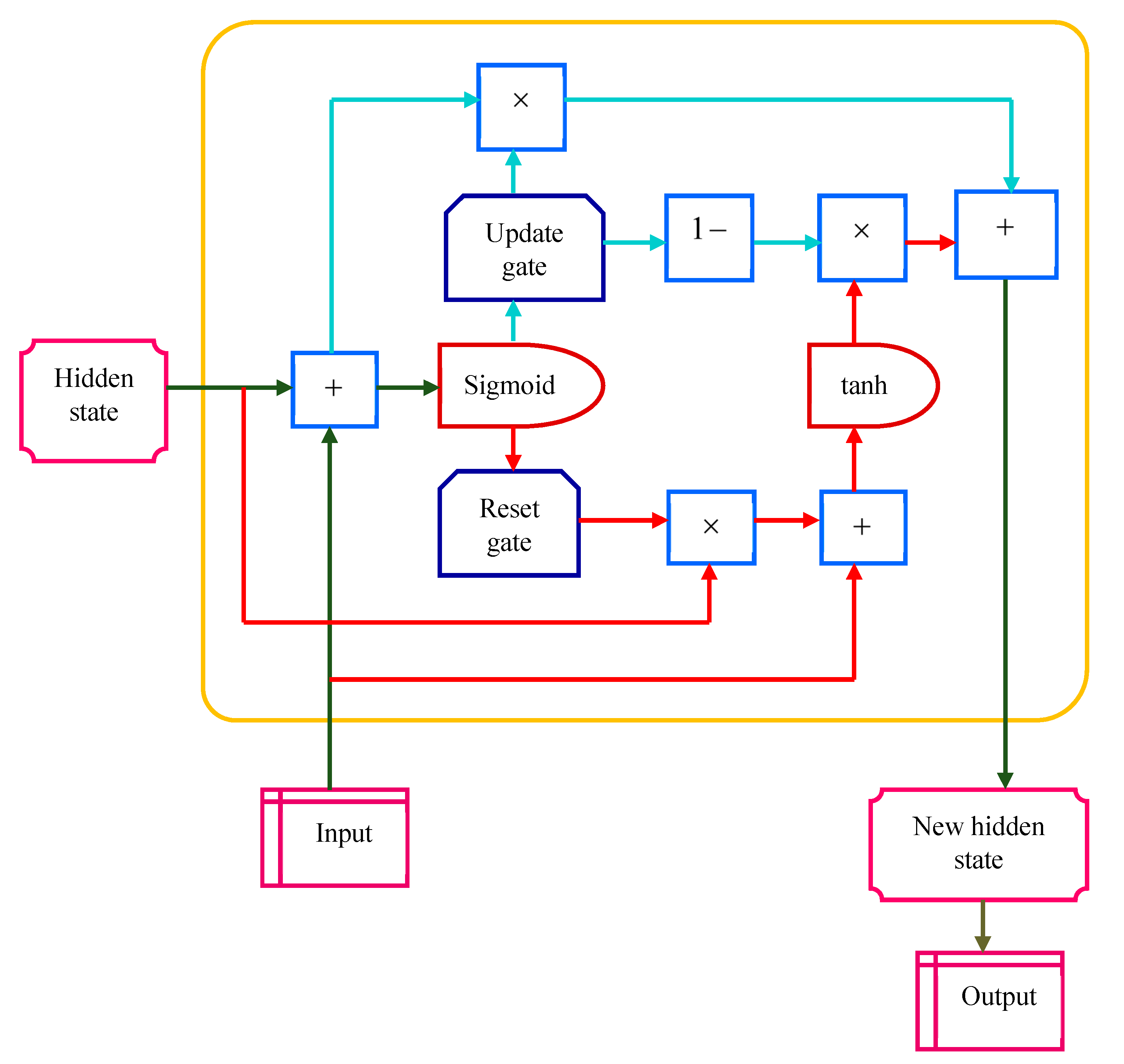
3.4.1. Structure of GRU

Usually, GRU [23] is a gating model in Recurrent Neural Network (RNN) and is better than Long Short-Term Memory (LSTM) and Conventional Neural Network (CNN). Moreover, it is not affected by vanish gradent issue. GRU is similar to LSTM, along with forget gate, although it has fewer parameters than LSTM because there is absence of output gate. Additionally, reset gate and update gate are utilized in GRU. In general, GRU utilizes internal memory capacity for accumulating and filtering the information based on their reset and update gates. GRU still has the disadvantages of slow convergence and low learning efficiency.
w e = χ J w · q e 1 , p e
d e = χ J w · q e 1 , p e
q ˜ e = tanh J · d e q e 1 , p e
q e = 1 w e · q e 1 + w e , q ˜ e
where p e indicates input vector, q e represents output vector, d e refers to reset gate vector, χ and tanh are activation functions and  w e implies update vector. The output of Sentiment Classification from GRU is denoted as V t . The structure of GRU is shown in Figure 2.

3.4.2. Training of GRU Based on Developed TD-Spider Taylor ChOA

The training process of GRU was performed using developed TD-Spider Taylor ChoA, which was newly introduced by incorporating TDO approach, SMO model, Taylor series and ChoA. Here, ChoA [25], SMO algorithm [26] and Taylor series [27] were incorporated with TDO algorithm to improve the performance in real world applications. Thus, the combination of the above-mentioned algorithms achieved better performance with regard to convergence speed, and effectively solved unconstrained and constrained issues. The algorithmic process of TD-Spider Taylor ChoA is illustrated as follows.
(a) Initialization: Originally, SMO generates the randomly dispersed population of spider monkey and is expressed by
S ( c ) = S min + S max + E ( 0 , 1 ) × S max S min
where S min and S max refer to minimum and maximum bounds and E(0,1) implies distributed random integer.
(b) Error Computation: Then, the fitness measure is calculated by Mean Square Error (MSE), in which, the fitness with minimal error is considered as best solution. The fitness measure is estimated by
ρ e = 1 m h = 1 m V t * V t 2
where V t * implies target output, m represents overall samples and  V t denotes classified output from GRU.
(c) Local Leader Phase: All spider monkeys vary their existing position depending on the details of local group member and local leader experience, which are expressed as
S ( c + 1 ) = S ( c ) + E ( 0 , 1 ) S a ( c ) S ( c ) + E ( 1 , 1 ) S r ( c ) S ( c )
where S ( c ) is current location of spider monkey, E ( 0 , 1 ) implies uniformly allocated random integer that ranges from 0 and 1, E ( 1 , 1 ) is consistently distributed random number among 1 and 1 and S r ( c ) refers to randomly selected spider monkey location.
(d) Global Leader Phase: Every updated location of spider monkey exploits practice of local group and global leader members in global leader section, which is illustrated as
S ( c + 1 ) = S ( c ) + E ( 0 , 1 ) S x ( c ) S ( c ) + E ( 1 , 1 ) S r ( c ) S ( c )
where S x ( c ) denotes location of global leader. Moreover, the updated expression of Spider Taylor-ChoA is specified as
S ( c + 1 ) = 5 S p r e j ( c ) [ 1 f s ] + f ( 4 , S ( c 1 ) S ( c 2 ) ) 5 2 f · 1 + S ( c ) 1 E ( 0 , 1 ) E ( 1 , 1 ) 2 E ( 0 , 1 ) E ( 1 , 1 ) + E ( 0 , 1 ) S x ( c ) + E ( 1 , 1 ) S r ( c ) 2 E ( 0 , 1 ) E ( 1 , 1 )
In order to solve the engineering problems, exploration phase of TDO algorithm was combined with Spider Taylor-ChoA. Here, condition 1 from exploration stage of TDO model was considered and is expressed as
S ( c + 1 ) = S ( c ) + v · ( P F · S ( c ) )
S ( c + 1 ) = S ( c ) + v · P v · F · S ( c )
S ( c + 1 ) = S ( c ) ( 1 v · F ) + v · P
S ( c ) = S ( c + 1 ) v · P ( 1 v · F )
Substituting Equation (24) in (20), we obtain
S ( c + 1 ) = 5 S p r e j ( c ) [ 1 f s ] + f l ( 4 S ( c 1 ) S ( c 2 ) ) 5 2 f · l + S ( c + 1 ) v · P ( 1 v · F ) 1 E ( 0 , 1 ) E ( 1 , 1 ) 2 E ( 0 , 1 ) E ( 1 , 1 ) + E ( 0 , 1 ) S x ( c ) + E ( 1 , 1 ) S r ( c ) 2 E ( 0 , 1 ) E ( 1 , 1 )
S ( c + 1 ) S ( c + 1 ) ( 1 v · F ) 1 E ( 0 , 1 ) E ( 1 , 1 ) 2 E ( 0 , 1 ) E ( 1 , 1 ) = 5 S p r e y ( c ) [ 1 f · s ] + f ( 4 S ( c 1 ) S ( c 2 ) ) 5 2 f · l v · P ( 1 v · F ) ]
S ( c + 1 ) ( 1 v · F ) ( 2 E ( 0 , 1 ) E ( 1 , 1 ) ) S ( c + 1 ) ( 1 E ( 0 , 1 ) E ( 1 , 1 ) ) ( 1 v · F ) · ( 2 E ( 0 , 1 ) E ( 1 , 1 ) ) = 5 . S p r e y ( c ) [ 1 f · s ] + f l ( 4 S ( c 1 ) S ( c 2 ) ) 5 2 f · l v · P ( 1 v · F ) 1 E ( 0 , 1 ) E ( 1 , 1 ) 2 E ( 0 , 1 ) E ( 1 , 1 ) + E ( 0 , 1 ) S x ( c ) + E ( 1 , 1 ) S r ( c ) 2 E ( 0 , 1 ) E ( 1 , 1 )
S ( c + 1 ) ( 1 v · F ) ( 2 E ( 0 , 1 ) E ( 1 , 1 ) ) 1 + E ( 0 , 1 ) + E ( 1 , 1 ) ( 1 v · F ) · ( 2 E ( 0 , 1 ) E ( 1 , 1 ) ) = S p v y ( c ) [ 1 f . s ] + f ( 4 S ( c 1 ) S ( c 2 ) ) 5 2 f · l v · P ( 1 v · F ) 1 E ( 0 , 1 ) E ( 1 , 1 ) 2 E ( 0 , 1 ) E ( 1 , 1 ) + E ( 0 , 1 ) S x ( c ) + E ( 1 , 1 ) S r ( c ) 2 E ( 0 , 1 ) E ( 1 , 1 )
S ( c + 1 ) = ( 1 1 + E ( 0 , 1 ) + E ( 1 , 1 ) ) ( 1 v · F ) · ( 2 E ( 0 , 1 ) E ( 1 , 1 ) ) 5 S p c y ( c ) [ 1 f . s ] + f ( 4 S ( c 1 ) S ( c 2 ) ) 5 2 f · l v · P ( 1 v · F ) 1 E ( 0 , 1 ) E ( 1 , 1 ) 2 E ( 0 , 1 ) E ( 1 , 1 ) + E ( 0 , 1 ) S x ( c ) + E ( 1 , 1 ) S r ( c ) 2 E ( 0 , 1 ) E ( 1 , 1 )
where s refers to coefficient vector, location of chimp at iteration c 1 is depicted as S ( c 1 ) , position of chimp at iteration c 2 is signified as S ( c 2 ) , S p r e y implies position of vector prey and l represents chaotic value.
(e) Global leader learning segment: Here, global leader location was updated through exploiting greedy selection model in population. Moreover, the spider monkey location with lower error rate was selected as updated global leader location.
(f) Local leader learning segment: In this section, location of local leader was updated through applying greedy selection in specific set, wherein the spider monkey with lowest error rate was chosen as updated location of local leader.
(g) Local leader decision section: If the location of any local leader is not updated to a particular threshold, then every member of specific set updates their location either by random initialization or through the utilization of integrated information from local and global leader, which is expressed by
S ( c + 1 ) = S ( c ) + E ( 0 , 1 ) S x ( c ) S ( c ) + E ( 0 , 1 ) S ( c ) S i ( c )
(h) Global leader decision phase: Here, global leader location was considered and, if it is not updated to particular iterations, then the global leader separates the population into small sets.
(i) Error re-computation: The fitness measure was calculated for every solution in which the least value is taken as optimal solution for sentiment classification.
(j) Termination: The above steps were continually processed until the best solution was obtained. Algorithm 1 provide the pseudo code of proposed TD-Spider Taylor ChOA.
Algorithm 1 Pseudo-code of proposed TD-Spider Taylor ChOA.
     Input: Population of spider monkey S
     Output: Optimum solution
Begin
Initialize the population randomly
Evaluate fitness rate based on expression (17)
Select the local and global leader using greedy selection method.
While (stopping norm is not fulfilled) do
Formulate new position with local leader using Equation (18)
Produce novel position with global leader through Equation (29)
Re-compute the fitness measure by using Equation (17)
Perform greedy selection scheme and choose the optimum one
Compute the probability of every member
Produce the new location of each group member
Update global and local position of leader
Redirect every member by Equation (30) when local group leader does not update position.
If global leader has not updated the location, then separate the group into small groups.
End while
Return the best solution
End

3.5. Review Rating Prediction

The extracted features were fed to HAN for executing Review Rating Prediction. In addition, HAN model was trained using developed Jaya-TDO technique to enhance the prediction performance.

3.5.1. Architecture of HAN

HAN [24] model comprises several elements, namely word attention, sentence attention layer, sentence encoder and word encoder. This network considers an extracted feature D g as input for Review Rating Prediction process.
(a) Word encoder: The input D g was embedded to vectors based on the embedding matrix F. In addition, bidirectional Gated Recurrent Unit (GRU) was applied to obtain word annotations through data summarizing from both the directions for signal. However, bidirectional GRU includes forward GRU, which reads features from first to last, whereas backward GRU reads features from last to first.
A = F D g · ; D g [ 1 , , Y ]
m = G R U ( A ) , D g [ 1 , Y ]
m ¯ = G R U ( A ) , D g [ Y , 1 ]
Here, annotation was attained for given data augmentation output D g by combining forward hidden state m and backward hidden state m so that m = [ m , m ] .
(b) Word attention: Every word does not uniformly contribute to sentence meaning representation. Conversely, attention component was devised to extracts words, which are important in a sentence. The representation of instructive features was combined to generate sentence vector.
z p = tanh ( F · m + o )
ρ = exp z p J z E Q exp z p J z E
E = ρ · m
Originally, word annotation m was subjected to one-layer MLP to acquire z p as the hidden representation of m; after that, significance of word as the correspondence of z p was computed with word-level context vector z E and normalized weight ρ was attained based on softmax function. Afterward, the sentence vector E was estimated using a weighted sum of word annotation by considering weights. Consequently, the context vector z E was observed as the high-level representation of the instructive word. The word context vector was randomly initialized and learned mutually in the training process. The architectural model of the HAN classifier is depicted in Figure 3.
(c) Sentence encoder: The document vector was derived and the bidirectional GRU was employed for encoding the sentences with sentence vector.
m f = G R U ( E )
m f = G R U ( E )
The sentence annotation was attained by concatenating m f and m f . Here, m f [ f m = m f , m f ] summarized nearby sentences about the sentences.
(d) Sentence attention: In sentence attention, a sentence-level context vector L is employed to identify sentence significance.
z f = tanh F I m f + o I
η f = exp z f J V f exp z f J V
Z = f η f · m f
where Z signifies document vector, which includes text information in a document. The final review rating predicted output of the HAN classifier is denoted as R t .

3.5.2. Training Process of HAN Using Developed Jaya-TDO Approach

The training procedure of HAN was completed by Jaya-TDO technique, which was newly developed by combining Jaya optimization [28] and TDO approach [29]. TDO model is bio-inspired metaheuristic model, and it is designed based on the characteristics of Tasmanian devil. This model efficiently resolves real word issues, even though it did not resolve optimization issues; thus, Jaya optimization was united with TDO. The algorithmic procedure of Jaya-TDO technique is defined below.
(a) Initialization: The initial population of Tasmanian devils is randomly produced depending on problem constraints. Here, population members of TDO recommended candidate rates for problem variables according to their search space location. Thus, every fellow of the population is a vector, along with amount of elements similar to the quantity of problem variables mathematically. The TDO members are expressed by the following matrix:
D = D 1 D i D A A × v = d 1 , 1 d 1 , y d 1 , v d j , 1 d j , y d j , v d A , 1 d A , y d A , v A × v
where D represents the population of Tasmanian devils, D i implies ith candidate solution, d j , y refers to candidate rate for yth variable, A indicates number of penetrating Tasmanian devils and v specifies quantity of variables for definite problems.
(b) Fitness computation: Afterwards, the fitness rate was calculated for every solution, in which, the fitness with lower value was specified as optimal solution and the fitness rate was evaluated by
ρ h = 1 m h = 1 m R t * R t 2
where R t * indicates target output, m denotes whole samples and R t signifies classified output from HAN.
(c) Exploration phase: The Tasmanian devil needs to feed on flesh rather than the hunting process. The behavior of the Tasmanian devil in the territory-scanning portion when identifying the meat is similar to the algorithm search process in solving space. Tasmanian devil identifies TDO exploration power, scanning different portions of search space to find real optimum portion. In search space, the position of other population members is considered as a carrion location for Tasmanian devil. Here, accidental selection of these situations was simulated by following equation in which uth population member is selected as target carrion for pth Tasmanian devil. Therefore, u must be selected randomly from 1 to T, whereas the reverse is p.
B u = L p ; u = 1 , 2 , , T ; p { 1 , 2 , , T p u }
where B u indicates selected carrion through pth Tasmanian devil. The new position was estimated for Tasmanian devil in search space based on selected carrion. The Tasmanian devil shifts to carrion when objective function is improved; otherwise, it transfers away from carrion. Additionally, Tasmanian devil motion technique is expressed by
d s , y new , R 1 = d s , y + z · v s , y C · d s , y ; O B u < O u d s , y + z · d s , y v s , y ; Otherwise
The position is recognized if objective function rate is enhanced in new location; otherwise, preceding position is chosen, which is illustrated as
L u = L u n e w , R 1 ; O u n e w , R 1 < O u L u ; otherwise
The 1st condition was taken from Equation (45) for updating process:
d s , y ( c + 1 ) = d s , y ( c ) + z · v s , y C · d s , y ( c )
d s , y ( c + 1 ) = d s , y ( c ) + z · v s , y z · C · d s , y ( c )
d s , y ( c + 1 ) = d s , y ( c ) ( 1 z · C ) + z · v s , y
From Jaya optimization,
d s , y ( c + 1 ) = d s , y ( c ) + z 1 d s , b e s t ( c ) d s , y ( c ) z 2 d s , worst ( c ) d s , y ( c )
Let us assume that d s , y ( c ) is positive; thus,
d s , y ( c + 1 ) = d s , y ( c ) + z 1 d s , best ( c ) d s , y ( c ) z 2 d s , worst ( c ) d s , y ( c )
d s , y ( c + 1 ) = d s , y ( c ) + z 1 d s , b e s t ( c ) z 1 d s , y ( c ) z 2 d s , worst ( c ) + z 2 d s , y ( c )
d s , y ( c + 1 ) = d s , y ( c ) 1 z 1 + z 2 + z 1 d s , best ( c ) z 2 d s , worst ( c )
d s , y ( c ) = d s , y ( c + 1 ) z 1 d s , b e s t ( c ) + z 2 d s , w o r s t ( c ) 1 z 1 + z 2
Substituting Equation (54) into (49),
d s , y ( c + 1 ) = d s , y ( c + 1 ) z 1 d s , b e s t ( c ) + z 2 d s , w o r s t ( c ) 1 z 1 + z 2 ( 1 z · C ) + z · v s , y
d s , y ( c + 1 ) d s , y ( c + 1 ) 1 z 1 + z 2 ( 1 z · C ) = z 2 d s , worst ( c ) z 1 d s , b e s t ( c ) 1 z 1 + z 2 ( 1 z · C ) + z · v s , y
d s , y ( c + 1 ) 1 z 1 + z 2 d s , y ( c + 1 ) ( 1 z · C ) 1 z 1 + z 2 = z 2 d s , worst ( c ) z 1 d s , b e s t ( c ) 1 z 1 + z 2 ( 1 z · C ) + z · v s , y
d s , y ( c + 1 ) 1 z 1 + z 2 1 + z · C 1 z 1 + z 2 = z 2 d s , worst ( c ) z 1 d s , b e s t ( c ) 1 z 1 + z 2 ( 1 z · C ) + z · v s , y
d s , y ( c + 1 ) = 1 z 2 z 1 + z · C z 2 d s , worst ( c ) z 1 d s , best ( c ) ( 1 z · C ) + z · v s , y 1 z 1 + z 2
where d s , y ( c + 1 ) is position of sth solution in yth dimension at iteration c + 1 , d s , worst ( c ) refers to worst location of sth solution at iteration c, d s , best ( c ) implies best location of sth solution at iteration c, z 1 and z 2 are random integers, v s , y represents selected carrion by sth solution in yth dimension and C symbolizes random integer.
(d) Exploitation segment: Other feeding technique for Tasmanian devil is to hunt and eat prey, which has two stages in attacking. Initially, it selects and attacks the prey through the observation of specific area, and it hunts to break the prey and starts eating. Here, local search of search space is similar to prey regarding chasing of neighborhood in attack location. In general, Tasmanian devils have the capacity to exploit convergence for enhanced candidate solution. Furthermore, Tasmanian devils attack the prey in nearby antagonized area in order to simulate chasing.
(e) Re-estimation of the fitness value: The fitness rate was evaluated by Equation (43) for every iteration, and the least value was taken as optimal solution.
(f) Termination: Above process recurred continuously until best solution was accomplished.

4. Systems Implementation and Evaluation

In this section, we first present the datasets, then details about the experimental setup and baseline benchmarks and, finally, evaluation metrics are shown.

4.1. Description of Datasets

In order to evaluate our system, three datasets were used, namely IMDB, Yelp 2013 and Yelp 2014 [30] https://github.com/thunlp/NSC (accessed on 10 August 2022). Social media review datasets https://shorturl.at/ENRUW (accessed on 15 August 2022) were adapted for Sentiment Classification and review rating prediction.
In this dataset, a group of 25,000 high polar movie reviews was considered for testing and training, as well as assisting in predicting negative and positive attitudes. Moreover, this dataset comprises reviews of 38,063 restaurants and 201 hotels.

4.2. Experimental Setup

The method that we proposed was implemented in the Python programming language. Our networks were trained on NVIDIA GTX 1080 in a 64-bit computer with an Intel(R) Core(TM) i7-6700 CPU @3.4GHz, 16 GB RAM and Ubuntu 16.04 operating system.

4.3. Evaluation Metrics

The performance of the proposed method was analyzed by considering the evaluation measures, such as precision, recall and F-measure.
Precision: It is the proportion of true positives to overall positives, and the precision measure is expressed as
δ = A A + B
where δ specifies the precision, A denotes the true positives and B signifies the false positives.
Recall: Recall is a measure that defines the proportion of true positives to the summing up of false negatives and true positives, and the equation is given as
ω = A A + E
where the precision measure is signified as ω , and E symbolizes the false negatives.
F-measure: It is a statistical measure of the accuracy of a test or an individual based on the recall and precision, and is given as
F m = 2 δ ω δ + ω
where F m denotes F-measure.

4.4. Baseline Methods

In order to evaluate the effectiveness of the proposed framework, our method was compared with several existing algorithms, such as:
Sentiment Classification: Hierarchical Self-Attentive Convolution Network (HSACN) [31], Multichannel Deep Convolutional Neural Network (MCNN) [32], Demand-aware Collaborative Bayesian Variational Network (DCBVN) [33], Spider Taylor-ChOA-based RMDL [34], Spider Monkey Crow Optimization Algorithm (SMCA) [3], W2v+ Attention+Bi-GRU [17] and the proposed TD-Spider TaylorChOA-GRU.
Review Rating Prediction: CNN [35], DNN [36], Bi-GRU [37], CNN+LSTM [38], Spider Taylor-ChOA-based HAN [34], and Proposed Jaya-TDO-HAN.

5. Results and Discussion

The performance results of our proposed model are presented in this section. The results were compared with the previously introduced methods, which were tested on the same datasets.

5.1. Sentiment Classification

5.1.1. Results Based on IMDB Dataset

Table 1 represents a comparative analysis of the Sentiment Classification model for several performance metrics through altering training data. The analysis of TD-Spider TaylorChOA-GRU for the precision, recall and F-measure is listed below. In 80% of training data, the precision of the developed TD-Spider TaylorChOA-GRU is 0.935. The recall of TD-Spider TaylorChOA-GRU is 0.941 for 80% of training data. In addition, considering 80% of training data, the F-measure of the developed model is 0.938.
Figure 4 represents the accuracy and loss for the Sentiment Classification model. Accuracy means the degree to which a measurement is accurate in relation to its true value. Here, when the iteration increases, the accuracy also increases. Similarly, the consequence of a poor prediction is loss. When we increase the iterations, the loss is decreased. Hence, the proposed method provides a better performance.

5.1.2. Results Based on Yelp 2013 Dataset

Table 2 represents a comparative analysis of the Sentiment Classification model for several performance metrics through altering training data. The analysis of TD-Spider TaylorChOA-GRU for the precision, recall and F-measure is listed below. In 80% of training data, the precision of the developed TD-Spider TaylorChOA-GRU is 0.914. The recall of TD-Spider TaylorChOA-GRU is 0.925 for 80% of training data and, considering 80% of training data, the F-measure of the developed model is 0.920.
Figure 5 represents the accuracy and loss for the Sentiment Classification model. Here, when the iteration increases, the accuracy also increases. When the iteration is 300, the accuracy is 0.970. Similarly, when we increase the iterations, the loss is decreased. When the iteration is 300, the loss is 0.04. Hence, the proposed method provides a better performance.

5.1.3. Results Based on Yelp 2014 Dataset

Table 3 represents a comparative analysis of the Sentiment Classification model for several performance metrics through altering training data. The analysis of TD-Spider TaylorChOA-GRU for the precision, recall, and F-measure is listed below. In 90% of training data, the precision of the developed TD-Spider TaylorChOA-GRU is 0.952. The recall of TD-Spider TaylorChOA-GRU is 0.965 for 90% of training data and, considering 90% of training data, the F-measure of the developed model is 0.959.
Figure 6 represents the accuracy and loss for the Sentiment Classification model. When the iteration is 0, the accuracy is 0.611. Similarly, when the iteration is 0, the loss is 0.397. Hence, the proposed method provides a better performance.

5.1.4. Social Media App Review Dataset

Table 4 represents a comparative analysis of the Sentiment Classification model for several performance metrics through altering training data. The analysis of TD-Spider TaylorChOA-GRU for the precision, recall and F-measure is listed below. In 90% of training data, the precision of the developed TD-Spider TaylorChOA-GRU is 0.897. The recall of TD-Spider TaylorChOA-GRU is 0.906 for 90% of training data and, considering 90% of training data, the F-measure of the developed model is 0.902.
Figure 7 represents the accuracy and loss for the Sentiment Classification model. Here, the proposed method also has the highest accuracy and minimum loss.

5.2. Review Rating Prediction

5.2.1. Results Based on Yelp IMDB Dataset

Table 5 represents a comparative analysis of the Review Rating Prediction model for several performance metrics through altering training data. The analysis of TD-Spider TaylorChOA-GRU for the precision, recall and F-measure is listed below. In 70% of training data, the precision of the developed TD-Spider TaylorChOA-GRU is 0.897. The recall of TD-Spider TaylorChOA-GRU is 0.914 for 70% of training data and, considering 70% of training data, the F-measure of the developed model is 0.906.
Figure 8 represents the accuracy and loss for the Review Rating Prediction model. Figure 8a represents the accuracy curve and Figure 8b represents the loss curve. The accuracy increases with the increase in the iteration and the loss decreases with the increase in the iteration.

5.2.2. Results Based on Yelp 2013 Dataset

Table 6 represents a comparative analysis of the Review Rating Prediction model for several performance metrics through altering training data. The analysis of TD-Spider TaylorChOA-GRU for the precision, recall and F-measure is listed below. In 70% of training data, the precision of the developed TD-Spider TaylorChOA-GRU is 0.887. The recall of TD-Spider TaylorChOA-GRU is 0.885 for 70% of training data and, considering 70% of training data, the F-measure of the developed model is 0.886.
Figure 9 represents the accuracy and loss for the Review Rating Prediction model. When the iteration is 300, the accuracy is 0.970. When the iteration is 300, the loss is 0.030. The results show that the proposed method offers a good performance regarding review rating prediction.

5.2.3. Results Based on Yelp 2014 Dataset

Table 7 represents a comparative analysis of the Review Rating Prediction model for several performance metrics through altering training data. The analysis of TD-Spider TaylorChOA-GRU for the precision, recall and F-measure is listed below. In 90% of training data, the precision of the developed TD-Spider TaylorChOA-GRU is 0.925. The recall of TD-Spider TaylorChOA-GRU is 0.941 for 90% of training data and, considering 90% of training data, the F-measure of the developed model is 0.933.
Figure 10 represents the accuracy and loss for the Review Rating Prediction model. When the iteration is 0, the accuracy is 0.629. When the iteration is 0, the loss is 0.370. Here, both the testing accuracy and training accuracy of the proposed method is high in the 300th iteration. Hence, the proposed method yields a better performance.

5.2.4. Social Media App Review Dataset

Table 8 represents a comparative analysis of the Review Rating Prediction model for several performance metrics through altering training data. The analysis of TD-Spider TaylorChOA-GRU for the precision, recall and F-measure is listed below. In 90% of training data, the precision of the developed TD-Spider TaylorChOA-GRU is 0.841. The recall of TD-Spider TaylorChOA-GRU is 0.865 for 90% of training data and, considering 90% of training data, the F-measure of the developed model is 0.853.
Figure 11 represents the accuracy and loss for the Review Rating Prediction model. Figure 11a represents the accuracy curve, which indicates both the testing accuracy and training accuracy. Figure 11b represents the loss curve, which indicates both the testing loss and training loss.

6. Conclusions and Future Work

This work presents a hybrid-optimization-enabled deep learning method for Sentiment Classification and Review Rating Prediction. Here, Yelp 2013, Yelp 2014, IMDB and social media app review datasets were taken as the input. The feature extraction process is more imperative for further Sentiment Classification and Review Rating Prediction processes. The GRU model was employed for Sentiment Classification and the HAN model was applied for Review Rating Prediction. Furthermore, the HAN and GRU models were trained by the hybrid optimization algorithm to enhance the detection and classification process. The experimental results show that the TD-Spider TaylorChOA-GRU and Jaya-TDO-HAN models obtained better results than existing methods. The proposed Jaya-TDO technique attained a better performance of 0.9425, 0.9654 and 0.9538, and TD-Spider Taylor ChOA achieved 0.9524, 0.9698 and 0.9588 in terms of the precision, recall and F-measure. In the future, the developed Sentiment Classification and Review Rating Prediction model can be further improved by extracting other features.

Author Contributions

S.K.B. designed and wrote the paper; H.L. supervised the work; S.K.B. performed the experiments with advice from B.X., P.D.S. and D.K.J. organized and proofread the paper. All authors have read and agreed to the published version of the manuscript.

Funding

This research received no external funding.

Institutional Review Board Statement

Not applicable.

Informed Consent Statement

Not applicable.

Data Availability Statement

The data used in the experiments are publicly available. Details have been given in Section 4.1.

Acknowledgments

The authors appreciate and acknowledge anonymous reviewers for their reviews and guidance.

Conflicts of Interest

The authors declare no conflict of interest.

Abbreviations

The following abbreviations are used in this manuscript:
ChOAChimp Optimization Algorithm
DCBVNDemand-aware Collaborative Bayesian Variational Network
DÉCORDeep-Learning-Enabled Course Recommender System
DNNDeep Neural Networks
GRUGated Recurrent Unit
HSACNHierarchical Self-Attentive Convolution Network
LSTM  Long Short-Term Memory
MCNN  Multi-model Convolutional Neural Network
NLPNatural Language Processing
RMDLRandom Multi-model Deep Learning
RNNRecurrent Neural Network
TDOTasmanian Devil Optimization

References

  1. Khurana, D.; Koli, A.; Khatter, K.; Singh, S. Natural language processing: State of the art, current trends and challenges. Multimed. Tools Appl. 2022, 1–32. [Google Scholar] [CrossRef]
  2. Rajput, A. Natural language processing, sentiment analysis, and clinical analytics. In Innovation in Health Informatics; Elsevier: Amsterdam, The Netherlands, 2020; pp. 79–97. [Google Scholar]
  3. Chugh, A.; Sharma, V.K.; Kumar, S.; Nayyar, A.; Qureshi, B.; Bhatia, M.K.; Jain, C. Spider monkey crow optimization algorithm with deep learning for Sentiment Classification and information retrieval. IEEE Access 2021, 9, 24249–24262. [Google Scholar] [CrossRef]
  4. Zheng, T.; Wu, F.; Law, R.; Qiu, Q.; Wu, R. Identifying unreliable online hospitality reviews with biased user-given ratings: A deep learning forecasting approach. Int. J. Hosp. Manag. 2021, 92, 102658. [Google Scholar] [CrossRef]
  5. Basiri, M.E.; Nemati, S.; Abdar, M.; Cambria, E.; Acharya, U.R. ABCDM: An attention-based bidirectional CNN-RNN deep model for sentiment analysis. Future Gener. Comput. Syst. 2021, 115, 279–294. [Google Scholar] [CrossRef]
  6. Xia, Y.; Cambria, E.; Hussain, A.; Zhao, H. Word polarity disambiguation using bayesian model and opinion-level features. Cogn. Comput. 2015, 7, 369–380. [Google Scholar] [CrossRef]
  7. Chandra, Y.; Jana, A. Sentiment analysis using machine learning and deep learning. In Proceedings of the 2020 7th International Conference on Computing for Sustainable Global Development (INDIACom), New Delhi, India, 12–14 March 2020; pp. 1–4. [Google Scholar]
  8. Jemai, F.; Hayouni, M.; Baccar, S. Sentiment Analysis Using Machine Learning Algorithms. In Proceedings of the 2021 International Wireless Communications and Mobile Computing (IWCMC), Harbin, China, 28 June–2 July 2021; pp. 775–779. [Google Scholar]
  9. Zhou, X.; Liang, W.; Huang, S.; Fu, M. Social recommendation with large-scale group decision-making for cyber-enabled online service. IEEE Trans. Comput. Soc. Syst. 2019, 6, 1073–1082. [Google Scholar] [CrossRef]
  10. Zhou, X.; Liang, W.; Kevin, I.; Wang, K.; Shimizu, S. Multi-modality behavioral influence analysis for personalized recommendations in health social media environment. IEEE Trans. Comput. Soc. Syst. 2019, 6, 888–897. [Google Scholar] [CrossRef]
  11. Jin, N.; Wu, J.; Ma, X.; Yan, K.; Mo, Y. Multi-task learning model based on multi-scale CNN and LSTM for Sentiment Classification. IEEE Access 2020, 8, 77060–77072. [Google Scholar] [CrossRef]
  12. Liu, S.; Lee, I. Sequence encoding incorporated CNN model for Email document sentiment classification. Appl. Soft Comput. 2021, 102, 107104. [Google Scholar] [CrossRef]
  13. Jianqiang, Z.; Xiaolin, G.; Xuejun, Z. Deep convolution neural networks for twitter sentiment analysis. IEEE Access 2018, 6, 23253–23260. [Google Scholar] [CrossRef]
  14. Zainuddin, N.; Selamat, A.; Ibrahim, R. Hybrid Sentiment Classification on twitter aspect-based sentiment analysis. Appl. Intell. 2018, 48, 1218–1232. [Google Scholar] [CrossRef]
  15. Kalaivani, P.; Shunmuganathan, K. Feature reduction based on genetic algorithm and hybrid model for opinion mining. Sci. Program. 2015, 2015, 12. [Google Scholar] [CrossRef]
  16. Lai, S.; Xu, L.; Liu, K.; Zhao, J. Recurrent convolutional neural networks for text classification. In Proceedings of the Twenty-Ninth AAAI Conference on Artificial Intelligence, Austin, TX, USA, 25–30 January 2015. [Google Scholar]
  17. Li, L.; Yang, L.; Zeng, Y. Improving Sentiment Classification of restaurant reviews with attention-based bi-GRU neural network. Symmetry 2021, 13, 1517. [Google Scholar] [CrossRef]
  18. Alamoudi, E.S.; Alghamdi, N.S. Sentiment Classification and aspect-based sentiment analysis on yelp reviews using deep learning and word embeddings. J. Decis. Syst. 2021, 30, 259–281. [Google Scholar] [CrossRef]
  19. Feng, S.; Song, K.; Wang, D.; Gao, W.; Zhang, Y. InterSentiment: Combining deep neural models on interaction and sentiment for Review Rating Prediction. Int. J. Mach. Learn. Cybern. 2021, 12, 477–488. [Google Scholar] [CrossRef]
  20. Ahmed, B.H.; Ghabayen, A.S. Review Rating Prediction framework using deep learning. J. Ambient. Intell. Humaniz. Comput. 2020, 13, 3423–3432. [Google Scholar] [CrossRef]
  21. Sadiq, S.; Umer, M.; Ullah, S.; Mirjalili, S.; Rupapara, V.; Nappi, M. Discrepancy detection between actual user reviews and numeric ratings of Google App store using deep learning. Expert Syst. Appl. 2021, 181, 115111. [Google Scholar] [CrossRef]
  22. Hong, T.P.; Lin, C.W.; Yang, K.T.; Wang, S.L. Using TF-IDF to hide sensitive itemsets. Appl. Intell. 2013, 38, 502–510. [Google Scholar] [CrossRef]
  23. Santur, Y. Sentiment analysis based on gated recurrent unit. In Proceedings of the 2019 International Artificial Intelligence and Data Processing Symposium (IDAP), Malatya, Turkey, 21–22 September 2019; pp. 1–5. [Google Scholar]
  24. Yang, Z.; Yang, D.; Dyer, C.; He, X.; Smola, A.; Hovy, E. Hierarchical attention networks for document classification. In Proceedings of the 2016 Conference of the North American Chapter of the Association for Computational Linguistics: Human Language Technologies, San Diego, CA, USA, 12–17 June 2016; pp. 1480–1489. [Google Scholar]
  25. Khishe, M.; Mosavi, M.R. Chimp optimization algorithm. Expert Syst. Appl. 2020, 149, 113338. [Google Scholar] [CrossRef]
  26. Bansal, J.C.; Sharma, H.; Jadon, S.S.; Clerc, M. Spider monkey optimization algorithm for numerical optimization. Memetic Comput. 2014, 6, 31–47. [Google Scholar] [CrossRef]
  27. Mangai, S.A.; Sankar, B.R.; Alagarsamy, K. Taylor series prediction of time series data with error propagated by artificial neural network. Int. J. Comput. Appl. 2014, 89, 41–47. [Google Scholar]
  28. Rao, R. Jaya: A simple and new optimization algorithm for solving constrained and unconstrained optimization problems. Int. J. Ind. Eng. Comput. 2016, 7, 19–34. [Google Scholar]
  29. Dehghani, M.; Hubálovskỳ, Š.; Trojovskỳ, P. Tasmanian devil optimization: A new bio-inspired optimization algorithm for solving optimization algorithm. IEEE Access 2022, 10, 19599–19620. [Google Scholar] [CrossRef]
  30. Chen, H.; Sun, M.; Tu, C.; Lin, Y.; Liu, Z. Neural Sentiment Classification with user and product attention. In Proceedings of the 2016 Conference on Empirical Methods in Natural Language Processing, Austin, TX, USA, 1–5 November 2016; pp. 1650–1659. [Google Scholar]
  31. Zeng, H.; Ai, Q. A hierarchical self-attentive convolution network for review modeling in recommendation systems. arXiv 2020, arXiv:2011.13436. [Google Scholar]
  32. Da’u, A.; Salim, N.; Rabiu, I.; Osman, A. Recommendation system exploiting aspect-based opinion mining with deep learning method. Inf. Sci. 2020, 512, 1279–1292. [Google Scholar]
  33. Wang, C.; Zhu, H.; Zhu, C.; Zhang, X.; Chen, E.; Xiong, H. Personalized employee training course recommendation with career development awareness. In Proceedings of the Web Conference 2020, Taipei, Taiwan, 20–24 April 2020; pp. 1648–1659. [Google Scholar]
  34. Banbhrani, S.K.; Xu, B.; Lin, H.; Sajnani, D.K. Spider Taylor-ChOA: Optimized Deep Learning Based Sentiment Classification for Review Rating Prediction. Appl. Sci. 2022, 12, 3211. [Google Scholar] [CrossRef]
  35. Zhang, K.; Qian, H.; Liu, Q.; Zhang, Z.; Zhou, J.; Ma, J.; Chen, E. Sifn: A sentiment-aware interactive fusion network for review-based item recommendation. In Proceedings of the 30th ACM International Conference on Information & Knowledge Management, Online, 1–5 November 2021; pp. 3627–3631. [Google Scholar]
  36. Chambua, J.; Niu, Z. Review text based rating prediction approaches: Preference knowledge learning, representation and utilization. Artif. Intell. Rev. 2021, 54, 1171–1200. [Google Scholar] [CrossRef]
  37. Bu, J.; Ren, L.; Zheng, S.; Yang, Y.; Wang, J.; Zhang, F.; Wu, W. ASAP: A chinese review dataset towards aspect category sentiment analysis and rating prediction. arXiv 2021, arXiv:2103.06605. [Google Scholar]
  38. Shrestha, N.; Nasoz, F. Deep learning sentiment analysis of amazon. com reviews and ratings. arXiv 2019, arXiv:1904.04096. [Google Scholar]
Figure 1. An illustration of proposed framework for Sentiment Classification and review rating prediction.
Applsci 12 10292 g001
Figure 2. An illustration of Gated Recurrent Unit (GRU).
Applsci 12 10292 g002
Figure 3. An illustration of Hierarchical Attention Network (HAN).
Applsci 12 10292 g003
Figure 4. Performance analysis based on (a) accuracy and (b) loss for Sentiment Classification using IMDB dataset.
Applsci 12 10292 g004
Figure 5. Performance analysis based on (a) accuracy and (b) loss for Sentiment Classification using Yelp 2013 dataset.
Applsci 12 10292 g005
Figure 6. Performance analysis based on (a) accuracy and (b) loss for Sentiment Classification using Yelp 2014 dataset.
Applsci 12 10292 g006
Figure 7. Performance analysis based on (a) accuracy and (b) loss for Sentiment Classification using social media app review dataset.
Applsci 12 10292 g007
Figure 8. Performance analysis based on (a) accuracy and (b) loss for Review Rating Prediction using IMDB dataset.
Applsci 12 10292 g008
Figure 9. Performance analysis based on (a) accuracy and (b) loss for Review Rating Prediction using Yelp 2013 dataset.
Applsci 12 10292 g009
Figure 10. Performance analysis based on (a) accuracy and (b) loss for Review Rating Prediction using Yelp 2014 dataset.
Applsci 12 10292 g010
Figure 11. Performance analysis based on (a) accuracy and (b) loss for Review Rating Prediction using social media app review dataset.
Applsci 12 10292 g011
Table 1. Comparative analysis of Sentiment Classification for IMDB dataset in terms of precision, recall and F-measure.
MetricsData (%)HSACNMCNNDCBVN[3][34][17]Proposed
Precision60%0.7850.8250.8550.8690.8950.9000.904
70%0.8050.8350.8650.8880.9030.9080.914
80%0.8240.8540.8850.8980.9250.9290.935
90%0.8520.8740.9050.9270.9410.9430.949
Recall60%0.7950.8350.8650.8770.9050.9080.914
70%0.8140.8410.8850.8980.9140.9190.925
80%0.8410.8650.8950.9080.9370.9390.941
90%0.8650.8850.9140.9370.9650.9680.970
F-measure60%0.7900.8300.8600.8730.9000.9040.909
70%0.8090.8380.8750.8930.9080.9130.920
80%0.8330.8600.8900.9030.9310.9340.938
90%0.8590.8800.9100.9320.9530.9550.959
Table 2. Comparative analysis of Sentiment Classification for Yelp 2013 dataset in terms of precision, recall and F-measure.
MetricsData (%)HSACNMCNNDCBVN[3][34][17]Proposed
Precision60%0.7540.7750.8140.8250.8420.8480.857
70%0.7650.7850.8250.8480.8650.8680.875
80%0.7950.8140.8470.8650.9040.9080.914
90%0.8250.8410.8850.9070.9330.9380.947
Recall60%0.7750.7950.8330.8580.8750.8790.887
70%0.7850.7960.8540.8750.8960.8980.901
80%0.8010.8250.8750.8980.9140.9180.925
90%0.8330.8650.8950.9160.9410.9480.950
F-measure60%0.7650.7850.8230.8410.8580.8630.872
70%0.7750.7910.8400.8610.8800.8830.888
80%0.7980.8200.8600.8810.9090.9130.920
90%0.8290.8530.8900.9110.9370.9430.949
Table 3. Comparative analysis of Sentiment Classification for Yelp 2014 dataset in terms of precision, recall and F-measure.
MetricsData (%)HSACNMCNNDCBVN[3][34][17]Proposed
Precision60%0.7750.7990.8330.8580.8750.8780.887
70%0.7850.8040.8480.8650.8950.8990.905
80%0.8010.8240.8650.8840.9140.9180.925
90%0.8330.8540.8950.9170.9470.9500.952
Recall60%0.7850.8010.8540.8650.8850.8900.899
70%0.7950.8240.8750.8870.9050.9100.914
80%0.8140.8350.8850.8980.9250.9290.937
90%0.8480.8650.9030.9170.9550.9600.965
F-measure60%0.7800.8000.8430.8620.8800.8840.893
70%0.7900.8140.8610.8760.9000.9040.910
80%0.8080.8300.8750.8910.9200.9230.931
90%0.8400.8600.8990.9170.9510.9550.959
Table 4. Comparative analysis of Sentiment Classification for social media app review dataset in terms of precision, recall and F-measure.
MetricsData (%)HSACNMCNNDCBVN[3][34][17]Proposed
Precision60%0.7410.7690.8070.8160.8340.8480.858
70%0.7680.7850.8210.8370.8540.8650.875
80%0.7850.8070.8410.8590.8640.8750.887
90%0.7980.8140.8650.8690.8740.8870.897
Recall60%0.7540.7780.8140.8270.8410.8580.865
70%0.7780.7990.8290.8480.8620.8760.887
80%0.7980.8140.8320.8590.8780.8870.897
90%0.8010.8250.8480.8650.8870.8980.906
F-measure60%0.7480.7740.8110.8210.8380.8530.862
70%0.7730.7910.8250.8420.8580.8700.881
80%0.7910.8110.8370.8590.8710.8810.892
90%0.8000.8200.8560.8670.8810.8920.902
Table 5. Comparative analysis of Review Rating Prediction for IMDB dataset in terms of precision, recall and F-measure.
MetricsData (%)DNNCNN+LSTMBi-GRUCNN[3][34][17]Proposed
Precision60%0.6350.6850.7410.8450.8580.8650.8770.887
70%0.6480.7030.7650.8600.8690.8850.8890.897
80%0.6850.7450.7850.8850.8980.9190.9200.925
90%0.6950.7650.8050.9010.9160.9310.9370.943
Recall60%0.6540.6990.7540.8500.8690.8850.8890.897
70%0.6750.7140.7850.8700.8870.9050.9080.914
80%0.6950.7540.8040.9080.9160.9330.9380.941
90%0.7240.7750.8250.9280.9480.9540.9590.965
F-measure60%0.6450.6920.7480.8470.8630.8750.8830.892
70%0.6610.7080.7750.8470.8780.8950.8980.906
80%0.6900.7500.7950.8470.9070.9250.9290.933
90%0.7090.7700.8150.8470.9320.9430.9480.954
Table 6. Comparative analysis of Review Rating Prediction for Yelp 2013 dataset in terms of precision, recall and F-measure.
MetricsData (%)DNNCNN+LSTMBi-GRUCNN[3][34][17]Proposed
Precision60%0.6330.6650.7040.7990.8080.8410.8480.855
70%0.6540.6960.7370.8240.8480.8650.8750.887
80%0.6960.7330.7540.8650.8870.8950.9000.905
90%0.7410.7650.7990.8950.9090.9250.9280.933
Recall60%0.6540.6990.7410.8010.8260.8540.8590.865
70%0.6750.7140.7540.8350.8590.8750.8790.885
80%0.7140.7410.7850.8950.9000.9020.9080.915
90%0.7690.8040.8410.9010.9170.9350.9390.941
F-measure60%0.6430.6820.7220.8000.8170.8480.8530.860
70%0.6640.7050.7450.8300.8530.8700.8770.886
80%0.7050.7370.7690.8800.8930.8990.9040.910
90%0.7550.7840.8190.8980.9130.9300.9330.937
Table 7. Comparative analysis of Review Rating Prediction for Yelp 2014 dataset in terms of precision, recall and F-measure.
MetricsData (%)DNNCNN+LSTMBi-GRUCNN[3][34][17]Proposed
Precision60%0.6410.6950.7410.7850.8080.8410.8480.854
70%0.6850.7140.7650.8020.8370.8650.8690.875
80%0.7010.7750.8250.8650.8760.8950.9070.914
90%0.7250.7990.8410.8950.9080.9140.9190.925
Recall60%0.6650.7140.7540.8010.8360.8540.8590.866
70%0.7010.7320.7750.8140.8590.8750.8800.885
80%0.7140.7950.8330.8750.8880.9010.9080.914
90%0.7330.8140.8540.9120.9270.9330.9390.941
F-measure60%0.6530.7040.7480.7930.8210.8480.8530.860
70%0.6930.7230.7700.8080.8480.8700.8740.880
80%0.7080.7850.8290.8700.8820.8980.9070.914
90%0.7290.8060.8480.9040.9170.9230.9280.933
Table 8. Comparative analysis of Review Rating Prediction for social media app review dataset in terms of precision, recall and F-measure.
MetricsData (%)DNNCNN+LSTMBi-GRUCNN[34]Proposed
Precision60%0.6590.6780.7040.7540.7780.807
70%0.6780.6850.7250.7780.7990.814
80%0.6990.7140.7410.7890.8140.829
90%0.7010.7330.7540.7990.8250.841
Recall60%0.6780.6900.7150.7690.7850.814
70%0.6870.6990.7350.7780.7990.824
80%0.6990.7040.7450.7870.8140.848
90%0.7040.7150.7550.8070.8250.865
F-measure60%0.6680.6840.7090.7610.7820.811
70%0.6830.6920.7300.7780.7990.819
80%0.6990.7090.7430.7880.8140.838
90%0.7030.7230.7540.8030.8250.853
Publisher’s Note: MDPI stays neutral with regard to jurisdictional claims in published maps and institutional affiliations.

