Short-Term Segment-Level Crash Risk Prediction Using Advanced Data Modeling with Proactive and Reactive Crash Data

Abstract

Highway crashes, along with the property damage, personal injuries, and fatalities that they cause, continue to present one of the most significant and critical transportation problems. At the same time, provision of safe travel is one of the main goals of any transportation system. For this reason, both in transportation research and practice much attention has been given to the analysis and modeling of traffic crashes, including the development of models that can be applied to predict crash occurrence and crash severity. In general, such models assess short-term crash risks at a given highway facility, thus providing intelligence that can be used to identify and implement traffic operations strategies for crash mitigation and prevention. This paper presents several crash risk and injury severity assessment models applied at a highway segment level, considering the input data that is typically collected or readily available to most transportation agencies in real-time and at a regional network scale, which would render them readily applicable in practice. The input data included roadway geometry characteristics, traffic flow characteristics, and weather condition data. The paper develops, tests, and compares the performance of models that employ Random effects Bayesian Logistics Regression, Gaussian Naïve Bayes, K-Nearest Neighbor, Random Forest, and Gradient Boosting Machine methods. The paper applies random oversampling examples (ROSE) method to deal with the problem of data imbalance associated with the injury severity analysis. The models were trained and tested using a dataset of 10,155 crashes that occurred on two interstate highways in New Jersey over a two-year period. The paper also analyzes the potential improvement in the prediction abilities of the tested models by adding reactive data to the analysis. To that end, traffic crashes were classified in multiple classes based on the driver age and the vehicle age to assess the impact of these attributes on driver injury severity outcomes. The results of this analysis are promising, showing that the simultaneous use of reactive and proactive data can improve the prediction performance of the presented models.

1. Introduction

Ensuring traffic safety is one of the primary goals of highway transportation authorities. To better understand the causes and factors contributing to highway crashes, and identify the measures for improving highway safety, much of the traffic safety research focuses on developing a better understanding of how, why, when, and where the highway crashes occur. The outcomes of such studies can then be used to ascertain the likelihood of crash occurrence under the given conditions and take the appropriate actions to reduce the frequency or mitigate the crashes before they occur.

Conceptually, a variety of factors contribute to the crash occurrence (or likelihood of crash) and crash severity, including the factors related to driver performance, roadway characteristics, vehicle characteristics, and environmental conditions. Some data that can help ascertain these factors are known or can be monitored in real time. This data is known as proactive data. Examples of such data are road characteristics, road-weather and traffic condition data. The advances in intelligent transportation systems (ITS), especially in the areas of connected vehicle, vehicle telemetry, and remote sensing data collection technologies, have significantly improved the ability to analyze traffic and road performance. These technologies have provided opportunities to collect and analyze data in near-real-time and aggregated to relatively short roadway segment level, including the data on prevailing vehicle speeds and travel times, lane occupancy, and road-weather and environmental characteristics. However, the challenges in this respect remain as such data collection is often limited to critical roadway segments and major highway facilities, without providing the coverage at the regnal transportation network scale. Indeed, the literature review reveals that the existing studies of real-time crash risk prediction are based on the real-time traffic counts and density collected from Automatic Vehicle Identification (AVI) sensors and real-time weather data collected from weather stations. Due to the limitation in data availability, those models could only be applied to specific, well instrumented facilities or local networks, and would not be applicable as support systems for dynamic monitoring of crash risks (in terms of crash likelihood and severity) and regional traffic operations decision making.

Moreover, the findings of the previous studies [1,2,3] suggest that the driver and vehicle characteristics represent significant factors of crash occurrence and severity of crashes. The data about the drivers and vehicles involved in a crash is collected after the crash occurrence as part of crash investigation and reporting, which is why this data is often referred to as reactive crash data. Thus, it is challenging to ascertain the effect of driver performance and vehicle characteristics data in proactive crash risk models. Yet, Reiman and Pietikäinen [4] showed that using both reactive and proactive data can be more useful for the organizations and decision makers. This premise is confirmed by Sarkar et al. [5] in a study that demonstrated the effectiveness of using a combination of reactive and proactive data in predicting the injury severity of accidents in the workplace.

The impetus and motivation for this study is the interest in developing a modeling framework for segment-level crash risk prediction considering roadway geometry characteristics, traffic flow characteristics, and weather conditions (e.g., precipitation and visibility). In contrast to previous studies, this paper demonstrates application of crash prediction models using the data that is readily available at a regional road network scale, rather than considering data generally available only at specific, well-equipped, and data-rich roadway segments. The main shortcoming of the previous models calibrated using such datasets is that they cannot be applied in locations where such data is not available in real time or near-real time, which renders these models not applicable in regional traffic operations management. In addition, this study proposes a combined real-time crash severity prediction model that includes both proactive and reactive explanatory variables, thus closing the gap that exits in the current literature due to lack of consideration of reactive data in predictive crash models. The proposed approach examines the potential improvement in predictive performance of the injury severity models by incorporating the reactive data on driver age and vehicle age. The proposed modeling framework is implemented using a case study of two freeways in the State of New Jersey, United States. Several statistical and machine learning models were compared to find the most effective one based on the prediction performance metrics. In addition, the data sampling was employed including the matched case–control and random oversampling examples (ROSE) methods to address the data imbalance problem of the dataset.

2. Summary of the Literature Review

Numerous studies have been conducted that utilized advanced data analysis methods to assess the crash risk in real time. Statistical analysis and machine learning (ML) models are the most common methods used in real-time traffic crash risk and crash severity prediction research. These models highlight the identification of factors affecting traffic crash risk and severity. In fact, both statistical analysis and ML methods focus on the prediction capabilities and false alarm rate of real-time traffic crash risk prediction models. For instance, Xu, Tarko [6] developed a three-stage sequential binary logit model to predict crash likelihood along a 29-mile segment of the I-88 freeway in San Francisco. The model considered three severity levels and it was calibrated using 22 input variables derived from the data obtained from roadside detectors in 30 s intervals. The weather condition (clear vs. adverse weather) was considered as an additional explanatory variable. The model evaluation was performed using a 20-fold cross-validation, and the findings showed that the traffic flow characteristics contributing to crash likelihood were substantially different at each severity level.

Theofilatos [7] investigated accident likelihood by incorporating real-time traffic and weather data for urban arterials in Athens, Greece. The traffic and weather data were aggregated into 1 h intervals. For every crash case, two non-crash cases were identified for the same location and time interval, one week before and one week after the crash occurrence. The random forest (RF) method was used to select the significant variables, and the Bayesian logistic regression (BLR) was used to model the likelihood of crashes. The results showed that the crash likelihood is most impacted by the standard deviation of occupancy and the coefficient of variation of traffic flow.

Yu and Abdel-Aty [8] developed crash risk assessment models that could be applied in real time crash prediction. The models were tested using the data from a 15-mile freeway section of I-70 in Colorado. The study dataset included crash record data and real-time traffic data collected from roadside radar detectors. For each crash case, four non-crash cases were identified for the same location two weeks before and two weeks after the crash occurrence. The classification and regression tree (CART) method was used to select the significant variables. The modeling methods applied in this study included (i) Bayesian logistic regression with fixed-parameters, (ii) Bayesian random-parameter logistic regression considering the seasonal variation, (iii) Bayesian random-effect logistic regression considering segment level heterogeneity, (iv) Support Vector Machine (SVM) with linear kernel, and (v) SVM with Radial Basis Function (RBF) kernel. The results showed that the Bayesian logistic regression with fixed parameters and the SVM with RBF kernel performed better than the other models.

Wang et al. [9] proposed a crash prediction model for crashes occurring at the expressway ramps in Central Florida. The dataset used in model calibration and testing consisted of the crash records collected from the Florida DOT statewide crash database, traffic flow data, roadway geometry data, and weather condition data collected from the National Climate Data Center (NCDC). Two separate BLR models were developed for single-vehicle and multi-vehicle crashes. The study found that four variables were significant in both models, including logarithm of the vehicle count in 5 min intervals, ramp configuration, road surface condition, and visibility. The traffic speed was found to be significant only in the single-vehicle model.

Theofilatos et al. [10] conducted a comparative study of crash prediction models using several machine learning (ML) and deep learning (DL) methods, including k-nearest neighbor (KNN), Naïve Bayes, decision tree (DT), RF, SVM, and shallow neural network. The models were trained and tested using the crash data for an urban motorway in Greece. For the modeling purposes, each crash record was matched with two non-crash cases. The explanatory variables were derived from the traffic data and weather data obtained in real time and matched to the crash and non-crash cases based on the corresponding time and location. The models were compared based on the performance metrics including accuracy, sensitivity, specificity, and AUC (area under the receiver operating characteristic (ROC) curve). The study found that the DL model outperformed the ML models as it provided a relatively balanced performance among all metrics.

Furthermore, Guo et al. applied RF in identifying the most critical variables in crash risk analysis study. A logistic regression model was developed to predict the crash risk on freeways in China and ascertain the relationship between traffic flow and risky driving behavior [11]. Wang et al. provided systematic ML models to predict the driving risk based on the data of drivers involved in crashes in China. Four three-based ensemble learning approaches were implemented: a gradient boosting decision tree (GBDT), an extreme gradient boosting decision tree, and RF models. The results revealed that GBDT outperformed other methods with an acceptable average precision of 0.68 [12]. Regarding the crash severity prediction, Sameen and Pradhan compared the Recurrent Neural Network (RNN), Multilayer Perceptron (MLP), and Bayesian Logistic Regression (BLR) models in prediction of injury severity based on 1130 crash records from the North-South Expressway in Malaysia, occurring over six years. The results suggested that the RNN appeared to have better prediction performance than MLP and BLR [13]. In another study, Lin et al., applied RF and Extreme Gradient Boosting (XGBoost) methods to analyze severity of crashes involving teen drivers on rural roads in West Texas. The RF and XGBoost models were each developed using two coding methods: (a) label encoder and (b) one hot encoder. The label encoder assigns numerical values to the unrepeated categories and treats categories in data as ordered. The potential shortcoming of this encoding method is that it can assume the relationships between the categories due to their ordering. On the other hand, one hot encoder converts the categorical variable into a sparse binary matrix. The results of this study indicate that the combination of label encoder and XGBoost appeared to yield better accuracy and computation time [14]. Along the same line of thought, Zhang et al. compared the prediction performance of two discrete choice models and four ML models to predict the injury severity in crashes at freeway diverge areas in Florida. This study applied ordered probit (OP) model and multinomial logit model, in comparison to RF, KNN, SVM, and decision tree models. Higher prediction accuracies were obtained with ML models as compared to discrete choice models, with RF showing the best performance and OP performing the worst [15]. In another study, Wahab and Jiang investigated the factors of injury severity in motorcycle crashes in Ghana. The authors applied ML methods including RF, J48 Decision Tree, and instance-based learning with parameter k, as well as multinomial logit model (MNLM). A ten-fold cross-validation was used to validate the ML models. This study also demonstrated superior performance of the ML methods as compared to the MNLM, with RF having the highest accuracy and extrapolation ability among the models [16].

With regards to data sampling and handling of imbalanced data in crash analysis, Kim and Lym investigated the prediction performance of the eight ML classifiers with/without data balancing in a case study of crash injury severity in Ohio, U.S. They applied the logistic and ordered logistic regression, RF, and ordered RF models. The results reveal that inclusion of data balancing improves performance of predicting severe crashes, while implementing ordering nature to develop an ordered RF model without balancing seems to yield the highest prediction accuracy [17]. Fiorentini and Losa compared four crash severity prediction models, including random tree, RF, KNN, and logistic regression, by handling the data imbalance using random undersampling the majority class (RUMC) technique. Results show that RUMC-based models enhance the positive rate of identifying fatality and injury crashes compared to imbalanced models [18].

3. Methodological Background

This section introduces analysis methods used in this study. The methods are selected based on the literature review, and each method is briefly explained in the following subsections.

3.1. Random Effect Bayesian Logistic Regression

The random effects Bayesian logistic regression (RBLR) was applied in this study as one of the methods for modeling crash risks. The Bayesian logistic regression differs from the standard (frequentist) logistic regression in the treatment of coefficients—it assumes that the coefficients follow a random distribution, rather than being fixed. The main advantage of Bayesian approach is the ability to capture uncertainty (variability) in the measured phenomena that may not be captured in the sample. This is achieved by formulating the model parameters as random variables that follow assumed prior distributions derived from some (prior) information about the measured phenomenon. The resulting confidence region associated with each estimated parameter is equivalent to the confidence interval in standard regression analysis, but it also captures the unobserved variability in the model parameters, which may improve the accuracy of the estimates. As another advantage over the standard regression models, the Bayesian models can help avoid the odds ratio overfitting, especially in complex models with large number of parameters. problem.

In this study of traffic crashes, the response variable is binary with two outcomes: $y_i=1$ and $y_i=0$. In the crash likelihood model, “1” represents a crash event and “0” represents a non-crash case. In the crash severity model, “1” represents an injury/fatal crash, and “0” represents a property-damage-only (PDO) crash. The probabilities associated with the binary events are $p_i$ and $1-p_i$, respectively. Thus, applying the Bayes theorem, the RBLR is formulated as follows:

$$y_i~ Bernoulli\left(p_i\right)$$

(1)

$$logit\left(p_i\right)={\beta }_0+{\beta }_j{X}_j$$

(2)

where the probability of each observation ($y_i$) is assumed to follow Bernoulli distribution, $X_j$ is the vector of N explanatory variables (j = 1,…, N), ${\beta }_j$ is the vector of random coefficients (slopes) associated with the explanatory variables, and ${\beta }_0$ is the random intercept in the regression model. Both the intercept and slope coefficients follow specific prior random distributions.

In general, depending on the corresponding prior probability distributions, the coefficients can be categorized into two groups: informative priors and non-informative priors. The informative priors are used when prior information about the estimated coefficients or their possible values are known, while the non-informative priors are used when little or nothing is known about the values of the coefficients except a general functional form of the prior probability distribution (most often Normal distribution).

3.2. Random Forest (RF)

Random Forest (RF) is a non-parametric supervised learning method that can be applied in both regression and classification modeling. The basic idea of the RF method is to build an ensemble of decision trees (i.e., a forest), which are randomly created through a process called bagging [19]. The bagging process consists of two components: bootstrapping and aggregation. With bootstrapping, each decision tree is trained using a random subset of features (decision factors) for splitting the nodes, and a random sample of observations from the original dataset. Each tree will still be trained using the same sample size as the original dataset, but each one will be formed through a random sampling from the original dataset with replacement. The final estimation of the response variable is then achieved by aggregating the estimates (outputs) of all decision trees in the forest. In regression models the aggregation is accomplished as an average of the decision trees outputs, while in the classification models this is accomplished by majority voting, i.e., selecting the outcome generated by the majority of trees in the forest. The RF method produces a collection of relatively uncorrelated trees, which are used to derive the output, rather than deriving the output from a single decision tree. This addresses the problem of overfitting and sensitivity to the sample dataset, which is the main shortcoming of individual decision trees. The RF method is commonly applied in modeling and analysis of highway crashes [7,10].

The hyperparameters of the RF model that should be specified include the number of decision trees in the forest and the number of features that should be randomly selected to split the nodes in each tree (referred to as mtry). These hyperparameters are optimized in the tuning process so as to minimize the error of the estimate. In that context, an important feature of the RF algorithm is differentiation of the input dataset due to random sampling. Namely, due to the sampling method applied in the bootstrapping process approximately one third of the data is not selected for model training. This subset of input data is called out-of-bag (OOB) data [20]. The OOB data is used to test the RF model and calculate the error of the estimate (referred to as OOB error). The OOB error depends on the selection of hyperparameters. For example, smaller number of randomly selected features to split the nodes at each tree (mtry) reduces the correlation among the trees, which is desirable, but it also reduces the strength (predictive power) of individual trees. Therefore, the objective of the model tuning process is to select the hyperparameters so as to minimize the OOB error.

In addition to model tuning, the OOB data can be used to quantify the variable importance. This is accomplished by assessing the change in OOB error in response to individual exclusion of explanatory variables (features) from the OOB data, while keeping the other variables unchanged. The change in OOB error can be measured by Mean Decrease Accuracy (MDA) as an average change in error over all trees in the RF after the exclusion of the given feature [21]. Higher values of MDA indicate the greater relative importance of a variable.

3.3. Gradient Boosting Machine (GBM)

Similar to RF, the Gradient Boosting Machine (GBM) is an ensemble learning method that uses decision trees as the base learning units. In contrast to RF, which uses relatively large trees and develops prediction through bootstrapping and aggregation, the GBM uses small trees and applies the concept of boosting which improves the learning strength of learner trees in a sequential manner. The GBM algorithm starts with a “weak learner” decision tree that fits the data using a simple regression model, and then calculates the error of prediction, e.g., as prediction residuals. It then develops new trees in a sequence, each growing more complex by focusing on the harder to predict examples in the data so as to reduce the prediction error. The prediction error is calculated using a differentiable loss function, and the algorithm searches for the best error reduction tree along the gradient of the loss function. Each tree in the sequence is given a certain weight (called “learning rate”) equivalent to the step-size (multiplier) of the residuals along the gradient applied to the next tree. The number of trees and the learning rate are determined (optimized) along with other model parameters in the model tuning process. In the end, the algorithm produces a complex ensemble of trees, and the final prediction is made as a weighted prediction of all trees in the ensemble. The study presented in this paper uses the multinomial deviance as the loss function. The GBM has gained a lot of popularity in machine learning modeling due to recent advancements and improvements in the search algorithm and the sampling methodology.

3.4. K-Nearest Neighbor (KNN)

KNN is a supervised machine learning method that can also be used both for classification and regression. The KNN algorithm determines the class of each observation in the analysis dataset based on the classes (e.g., PDO, injury, or fatality in the crash severity analysis) of K closest observations (nearest neighbors). The closeness is measured using some function of distance in a multi-dimensional space, with each dimension representing an explanatory variable (e.g., speed, traffic volume, geometric design characteristics, etc.). In classification algorithms, the class of an observation is determined as a majority class among its K nearest neighbors; in regression algorithms the class is determined as an average of classes of the K nearest neighbors [22]. To execute the KNN algorithm, two parameters must be specified: the value of K (i.e., how many neighboring observations should be considered for classification or regression), and the distance function (e.g., how will the distance between the neighbors be determined). Small values of K may create a model that is too specific to the training dataset, leading to overfitting and rendering the model unfit to properly classify datasets other than the one used in training. Large values of K, on the other hand, may lead to a weak, overly generalized model, unbale to properly classify both the training and testing datasets. The value of K is therefore determined in an iterative process, in which different values of K are applied and the one that yields the best performance (e.g., achieves the highest accuracy of prediction) is selected for the model. As a rule of thumb, in classification models where there are only two classes, which is the case in this study, K should be odd to avoid ties [23]. As for the distance function, in this study the Euclidean distance was used, which is formulated as:

$$dist\left(x_i,x_j\right)=\sqrt{{\displaystyle \sum }_{k=1}^p{\left(x_{ik}-x_{jk}\right)}^2}$$

(3)

where $dist\left(x_i,x_j\right)$ denotes the distance between the observations $i$and $j$, and $x_{ik}$ and $x_{jk}$ are the values of the $K$th factor for $i$ and $j$, respectively.

3.5. Gaussian Naïve Bayes (GNB)

The Naïve Bayes (NB) algorithm is a supervised probabilistic classification method based on Bayes’ theorem. The NB method classifies the observations by calculating the conditional probability that they belong to a target class given the values of model features, as follows:

$$P\left(y|X\right)=\frac{P\left(X|y\right)P\left(y\right)}{P\left(X\right)}=\frac{P\left(y\right){{\displaystyle \prod }}_{i=1}^{n}P(x_i|y)}{P\left(X\right)}$$

(4)

where $P\left(y|X\right)$ denotes the posterior probability of the observation belonging to the class $y$ given the set of features $X$, $P\left(X|y\right)$ denotes the likelihood of feature X given the class $y$, and the $P\left(y\right)$ and $P\left(X\right)$ represent the prior probabilities of the occurrence of class $y$ and feature $X$ respectively, calculated from the training data. An important assumption in this method is the strong (naïve) independence among the model features $X$. Additionally, the denominator $P\left(X\right)$ does not depend on the class $y$ and the values of features $X$ are given, so the prediction only depends on the enumerator in the formula above. In the study presented in this paper the Gaussian Naïve Based (GNB) method is applied, which uses the Gaussian (normal) distribution for the likelihood functions of feature $X$ given class $y$:

$$P(x_i|y)=\frac{1}{\sqrt{2\pi {\sigma }_y{}^2}}exp\left(-\frac{{\left(x_i-{\mu }_y\right)}^2}{2{\sigma }_y{}^2}\right)$$

(5)

where the ${\mu }_y$ is the mean and ${\sigma }_y$ is the standard deviation of the likelihood function calculated for each feature in the training dataset using maximum likelihood. The GNB method has been used in various road safety studies [10,24].

3.6. Model Performance Criteria

The performance of models in this study was evaluated using the following performance measures:

$$\mathrm{Overall}\mathrm{accuracy}=\frac{TP+TN}{Total crashes}$$

(6)

$$\mathrm{Sensitivity}=\frac{TP}{TP+FN}$$

(7)

$$\mathrm{Specificity}=\frac{TN}{TN+FP}$$

(8)

where:

• TP = True positive value, defined as the number of crash cases in the crash likelihood model (or fatal/injury crashes in crash severity model) that are correctly predicted.
• TN = True negative value, defined as the number of non-crash cases in the crash likelihood model (or PDO crashes in the crash severity model) that are correctly predicted.
• FP = False positive value, defined as the number of non-crash cases that are falsely predicted as crash cases in the crash likelihood model (PDO crashes falsely predicted as fatal/injury crashes in the crash severity model).
• FN = False negative value, defined as the number of crash cases that are falsely predicted as non-crash cases in the crash likelihood model (fatal/injury crashes falsely predicted as PDO crashes in the crash severity model).

The AUC was also used to evaluate each model. The closer the values of each of these measures are to 1, the better the prediction performance.

4. Data Collection and Preparation

4.1. Study Dataset

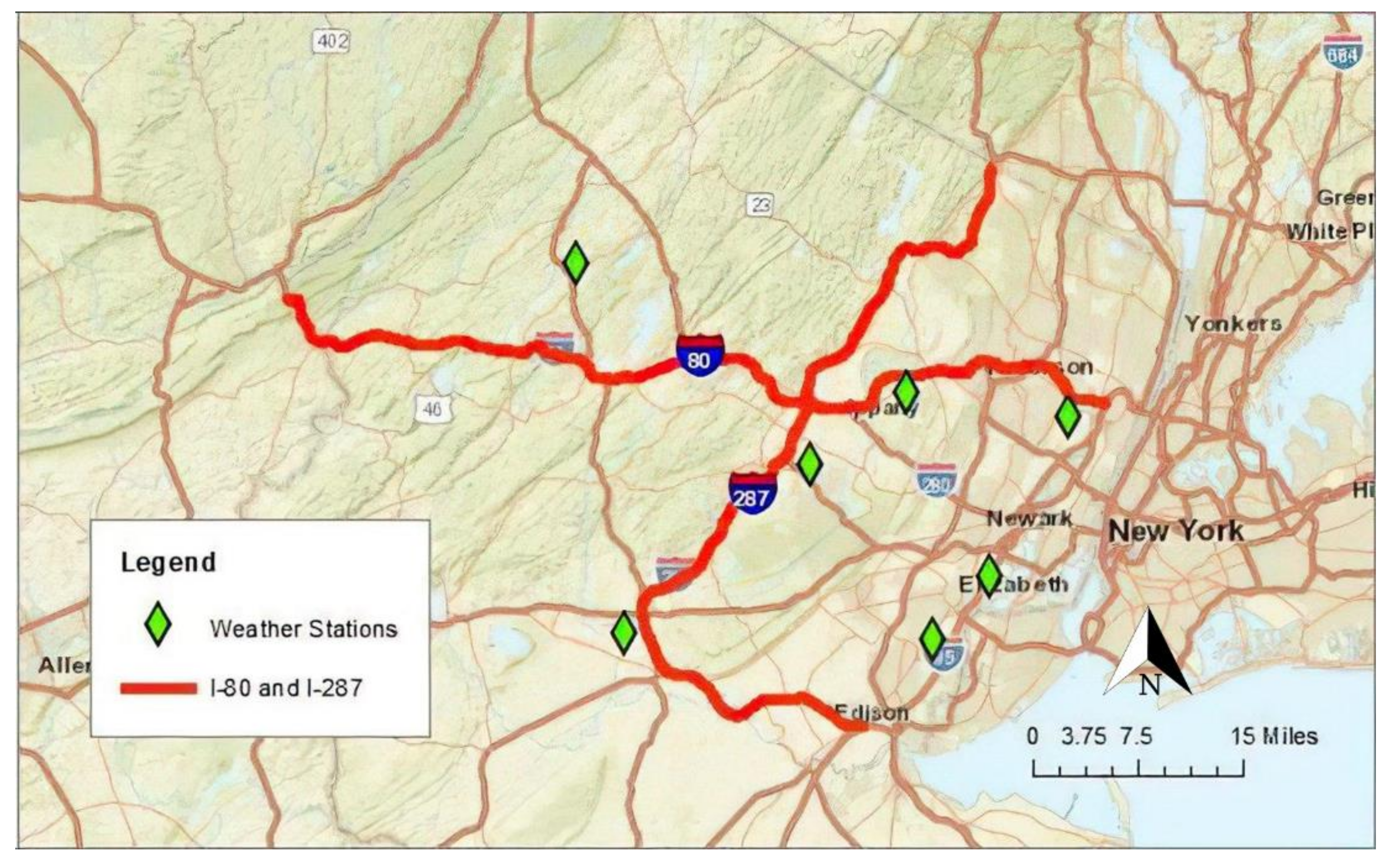
The study location included two interstate highways in New Jersey: the 68.5 miles long interstate I-80, which has a west-to-east alignment; and 67.5 miles long interstate I-287, which has a south-to-north alignment. The locations of I-80 and I-287 on the map of New Jersey along with the location of weather stations used in this study to collect the weather data are shown in Figure 1.

As stated before, the proactive data can be collected before the crash occurrence, ideally in near-real-time. The proactive data sources and datasets used in this study are readily available in real-time, at a roadway segment level, and for all sections of the major roadways in the State of New Jersey. The analysis dataset was compiled from the following sources: (a) New Jersey Department of Transportation (NJDOT) crash records database, which contains records of all reported highway crashes in the State of New Jersey; (b) NJDOT Congestion Management System (NJCMS), which provides estimated, synthesized hourly volume and volume-to-capacity ratio at a roadway segment level for all highways in NJDOT jurisdiction; (c) Prevailing vehicle speeds and travel times aggregated from the probe vehicles in 1 min increments at the roadway segment level, obtained from the Regional Integrated Transportation Information System (RITIS), (d) Historical weather observation data obtained from the Local Climatological Data (LCD) database for the weather stations managed by the National Weather Service (NWS).

The reactive data is collected after the crash occurrence and it provides additional details about the crash, such as vehicle and driver characteristics. The reactive data used in this study is contained in the statewide NJDOT crash records database, and it was used in the crash injury severity model only.

4.2. Data Integration

The study dataset included 10,155 crashes recorded from January 2017 to December 2018. Each crash record included the date and time of crash, as well as crash location as standard route identification (SRI), milepost, and direction, or as the latitude and longitude of the crash location that was matched to the SRI and milepost using the NJDOT roadway network GIS. The crash locations were matched to the corresponding NJCMS records (links) based on the SRI, the milepost range, and directionality defined for each NJCMS link. The matching NJCMS records provided the segment-level roadway characteristics, such as number of lanes and capacity, as well as traffic data such as hourly volumes and v/c ratios.

The traffic speed data at the crash location and the corresponding upstream and downstream segments was obtained from the RITIS dataset, in which the prevailing vehicle speeds are aggregated in 1-min increments for each Traffic Message Channel (TMC) link in the network. The TMC link definition tables for this study were obtained from NJDOT and they contained the Route ID, direction, and milepost range for each TMC link. This information, along with the timestamp of the reported speed, was used to associate the TMC link and the corresponding speed data with the crash records and NJCMS records. It should be noted that the limits of TMC do not coincide with the NJCMS roadway segments. Therefore, the TMC links had to be matched and conflated with the NJCMS segments in order match the speed records from the RITIS dataset to the roadway data and traffic volumes associated with the NJCMS segments. Having the speeds and volumes for consistent roadway segments (using NJCMS links as the bases), each crash record was then matched to the corresponding roadway segment.

To reduce the noise in the speed data and simulate the application of the models for crash prediction in traffic operation, each crash event was matched to 1 min speeds recorded over 10 min periods 5–15 min prior to the crash occurrence. For the modeling purposes, the 10 min average speed the standard deviation of speed, the coefficient of variation of speed, as well as average deviation from the speed limit was calculated for each of these 10 min period.

The weather data was collected from the LCD dataset and matched to each crash record based on the weather station location, date and time of the crash and the weather report. The shortest Euclidian distance was used to match the weather stations to NJCMS link associated with each crash, and by association to each crash in the analysis dataset. The weather data included hourly precipitation and hourly visibility observed during the hour of the crash. The weather stations used in this study (shown on the map in Figure 1) are all located at the regional airports.

Lastly, the effect of sun glare was assessed in this study as an additional factor of crash occurrence and severity. To assess the effect of sun glare, the position of the sun was estimated using Pysolar Python library [25] for each crash and non-crash case considering the crash location (i.e., it’s latitude and longitude), date and time (t). This procedure is illustrated in Figure 2.

As can be seen in Figure 2, the horizontal angle between the Sun and the vehicle can be calculated as:

$$h_{glare}=\left|\varnothing -\phi \right|$$

(9)

where $\varnothing$denotes the azimuth of the Sun, and $\phi$ denotes the horizonal angle of the roadway at the crash (non-crash) location relative to the East. Similarly, the vertical angle between the Sun and the vehicle can be calculated using the following equation:

$$v_{glare}=\left|\theta -{\theta }^{\prime }\right|$$

(10)

where $\theta$ denotes the sun elevation and $\theta ’$ denotes the slope of the roadway at the crash (non-crash) location. The horizontal and vertical angle of the roadway were assumed to reflect the corresponding horizontal and vertical angle of the vehicles traveling at the road segment at the time of crash (or non-crash event). The presence of sun glare affecting the driver was affirmed if the values of both $h_{glare}$ and $v_{glare}$ were less than 25°. Otherwise, it was assumed that there was no sun glare affecting the driver.

The summaries of the basic descriptive statistics of the datasets used in this study are provided in

Table 1. Summary of the roadway segment characteristics (including crash statistics).

Characteristic	I-287	I-80	Total
Number of crashes (total)	1267	8888	10,155
Number of injury/fatal crashes	236	1903	2139
Number of PDO crashes	1031	6985	8016
Roadway length (in miles)	67.5	68.5	136
Number of roadway segments (both ways)	116	164	280
Minimum length of a roadway segment (in miles)	0.020	0.100	0.020
Maximum length of a roadway segment (in miles)	5.140	4.020	5.140
Average length of a roadway segment (in miles)	1.218	0.936	1.053

and

Table 2. Summary of basic statistics for the continuous variables.

Variable	Min	Max	Mean	Median
CAPLINK	3268	8570	6138	6856
VC_RATIO	0.032	1.599	0.600	0.577
Vol16_Tr	0.032	1.450	0.576	0.554
HourlyPrecipitation	0.000	0.720	0.002	0.000
HourlyVisibility	0.000	74.00	8.898	10.00
speed_avg_1015	2.00	83.00	61.56	64.80
speed_sd_1015	0.00	25.23	1.29	0.89
speedup_dif_1015	0.00	63.00	8.72	6.20
speeddown_dif_1015	0.00	63.00	8.23	5.80

.

4.3. Explanatory Variables

The explanatory variables that were identified as the most critical and informative for crash likelihood and crash severity analysis are listed in

Table 3. Definition of the explanatory variables used in the study.

Variable	Type	Class	Source	Description
LANES	Categorical	Proactive	NJCMS	Number of lanes (the values are: 2, 3, 4, or 5)
Hour	Categorical	Proactive	NJCR	Time of the crash or non-crash (hour of the day)
Month	Categorical	Proactive	NJCR	Time of the crash or non-crash (month of the crash)
MEDIAN_TY	Binary	Proactive	NJCR	Median type (protected or non-protected)
Weekend	Binary	Proactive	NJCR	Day of the week (weekend of weekday)
Sun glare	Binary	Proactive	NJCMS	The effect of sun glare (0 = no effect, or 1 = Sun glare existed)
CAPLINK	Continuous	Proactive	NJCMS	Link capacity (vehicles/hour)
VC_RATIO	Continuous	Proactive	NJCMS	Volume-to-capacity ratio at the highway section during a given hour of the day and month [unitless]
Vol16_Tr	Continuous	Proactive	NJCMS	Hourly truck volume ratio
Hourly Precipitation	Continuous	Proactive	NWS	Hourly precipitation at the highway section during the hour of the crash or non-crash event obtained from the weather records for the closest weather station [inches/hour]
Hourly Visibility	Continuous	Proactive	NWS	Hourly visibility at the highway section during the hour of the crash or non-crash event obtained from the weather records for the closest weather station [miles]
speed_avg_1015	Continuous	Proactive	RITIS	Average speed at the highway section [miles/hour]. It is calculated for each crash and non-crash event as an average of 1 min prevailing speeds for the pertinent highway section over a 10 min period (5–15 min) prior to the crash or non-crash event.
speed_sd_1015	Continuous	Proactive	RITIS	Standard deviation of speed at the cash location [miles/hour]. It is calculated as a standard deviation of 1 min prevailing speeds for the pertinent highway section over a 10 min period (5–15 min) prior to the crash or non-crash event.
speedup_sd_1015	Continuous	Proactive	RITIS	Standard deviation of speed at the upstream highway section [miles/hour]. It is calculated as a standard deviation of 1 min prevailing speeds for the pertinent highway section over a 10 min period (5–15 min) prior to the crash or non-crash event.
speeddown_sd_1015	Continuous	Proactive	RITIS	Standard deviation of speed at the downstream highway section [miles/hour]. It is calculated as a standard deviation of 1 min prevailing speeds for the pertinent highway section over a 10 min period (5–15 min) prior to the crash or non-crash event.
speedup_dif_1015	Continuous	Proactive	RITIS	Deviation of speed from the speed limit [miles/hour] at the upstream roadway segment. Calculated as the difference between the average speed (speed_avg) and the speed limit (obtained for the upstream roadway segment from the NJCMS dataset).
speeddown_dif_1015	Continuous	Proactive	RITIS	Deviation of speed from the speed limit [miles/hour] at the downstream roadway segment. Calculated as the difference between the average speed (speed_avg) and the speed limit (obtained for the downstream roadway segment from the NJCMS dataset).
Shape_Leng	Continuous	Proactive	RITIS	Length of the highway segment [miles]
Age	Categorical	Reactive	NJCR	Driver’s age in years (the classes are defined as: age ≤ 25, 25 < age ≤ 60, and age > 60)
Veh_age	Categorical	Reactive	NJCR	Vehicle age in years (the classes are defined as: 0 < age ≤ 5, 5 < age ≤ 10, and age > 10)

.

4.4. Generating Non-Crash Cases for the Crash Likelihood Modeling

In the crash likelihood model the matched case-control methodology was used to introduce the non-crash cases to match the crash cases. The methodology is implemented by generating four non-crash cases for each crash at the same location, day of the week, and time-of-day: one case in the week before, one case two weeks before, one case in the week after, and one case two weeks after the corresponding crash occurrence. The 1:4 ratio of crash cases to non-crash cases were selected based on Ahmed and Abdel-Aty [27] who found this ratio to provide slightly better results when compared to other ratios of crash-to-non-crash cases. It should be noted that the matched case-control method employed in this study accounted for the confounding effects of the location (with the corresponding roadway characteristics) and time on crash occurrence. The other factors, such as vehicle, driver, weather and road condition parameters at the time of crash were not considered when generating non-crash cases for the analysis. After completing this step, the study dataset for the crash likelihood model had additional 40,620 records representing non-crash cases (in addition to the 10,155 crash records).

4.5. Correlation between the Explanatory Variables

Before proceeding with model estimation, it is important to check for correlation between the explanatory variables in the analysis dataset. The correlation was analyzed using the Pearson correlation coefficient matrix. Based on the correlation matrix, it was decided to exclude from further consideration the highway capacity (CAPLINK variable) as it was correlated with the number of lanes (LANES variable). The hourly volume (VOL variable) was also excluded from the models as it was correlated with the v/c ratio (v_ratio variable).

4.6. Determination of Significant Variables

The relative importance (significance) of explanatory variables was determined using an RF model, using MDA (Mean Decrease Accuracy) as the criterion of relative variable importance. The ranking of the relative variable importance is shown graphically in Figure 3 for both the crash likelihood model and the crash severity model. The vertical red (cordon) lines denote the separation between the significant variables to be considered (to the right of the cordon line) and variables that should be excluded as insignificant (to the left of the cordon line). The cordons were determined where the gap between variables was relatively large in terms of MDA.

It should be noted that in an attempt to include more parameters as models’ input, it was decided to use the second largest gap between the variables, in terms of MDA, to include (or eliminate) the variables in consideration. The literature suggests that models such as RF and GBM, are not affected by the inclusion of insignificant variables [20]. In RF, in general, nodes with the greatest decrease in impurity are found at the start of the trees, while nodes with the least decrease in impurity occur at the end of trees. Thus, the less important nodes have little effects on the models’ performance.

In both models the variables SHOULDER, Sunglare, Weekend, and MEDIAN_TY were not significant. Furthermore, the plots in Figure 3 suggested that HourlyPrecipitation and LANES should be omitted from the crash likelihood and crash severity models, respectively, due to their low relative importance.

4.7. Dealing with the Data Imbalance Problem

To overcome the problem of low frequency of fatal crashes, for the modeling purposes they were combined in a single class with injury crashes. However, even after combining the injury and fatal crashes, it was found that non-injury crash class accounted for 79% of the cases (8016 non-injury or PDO crashes out of the total of 10,155 crashes in the dataset). This may present a problem in model training: the traditional accuracy maximizer techniques may not perform adequately with the training dataset containing skewed distribution of classes, as they generally tend to perform better in favor of the majority class. In such situations it is advantageous to apply certain data transformations that result in a more balanced training dataset.

This study applied relatively novel Random Oversampling Examples (ROSE) method to resample and balance the initial training dataset. The ROSE method employs a random bootstrapping technique introduced by Menardi and Torelli [28], which can alleviate the data imbalance issue in binary classification problems. The method combines random oversampling and random undersampling by generating new artificial instances of data examples in the original classes using a smoothed bootstrapped approach [29].

Consider a training set of size n, consisting of a binary response variable $y$, with class labels $Y_j$ and a set of input data for each class, $x_{ij}, i=1,\dots , n_j$, where $n_j<n$ is the number of cases in class j. For each x belonging to the class $Y_j$, ROSE generates samples from a multivariate kernel density estimate of $f(x | y=Y_j)$ as follows:

$$\widehat{f(}x | y=Y_j)={\displaystyle \sum }_{i=1}^{n_j}{p}_{i}Pr (x | x_{ij})={\displaystyle \sum }_{i=1}^{n_j}\frac{1}{n_j} K_{H_j}\left(x-x_{ij}\right)$$

(11)

where $K_{H_j}$ denotes an estimated kernel function, and it’s smoothing matrix $H_j$ is defines as:

$$H_j=diag\left(h_1^{\left(j\right)}, \dots , h_d^{\left(j\right)}\right)$$

(12)

where d denotes the number of explanatory variables and

$$h_q^{\left(j\right)}={\left(\frac{4}{\left(d+2\right)n}\right)}^{1/\left(d+4\right)}{\widehat{\sigma }}_q^{\left(j\right)}, q=1, \dots , d$$

(13)

where ${\widehat{\sigma }}_q^{\left(j\right)}$ is the estimated standard deviation of the q-th variable. According to Bowman and Azzalini [30], the smoothing matrix minimizes the Asymptotic Mean Integrated Squared Error, assuming that the true conditional densities of the data follow Normal distribution. The practical implementation of ROSE encompasses the following steps:

• select $y^{*}=Y_j$ with probability ${\pi }_j$;
• select x such that $y_k=y^{*}, k=1, \dots , n$ with probability $\frac{1}{n_j}$;
• sample $x^{*}$ from the estimated kernel function.

Repeating steps 1 to 3 yields a newly generated training set of size m, with the probability of each class being ${\pi }_j$. Menardi and Torelli [28] showed that ROSE outperformed other well-known oversampling methods, such as synthetic minority oversampling technique (SMOTE), measured by higher values of the AUC in models implementing logistic regression and classification trees. This was the main motivation for implementing ROSE method, given the similar class of models employed in his study.

4.8. Final Preparation of the Training and the Testing Datasets

The input datasets for both crash likelihood and crash severity models were split into two subsets: (a) training dataset, which was used to train the models and contained 75% of features (data records), and (b) testing dataset, containing 25% of features. The training and testing datasets were separated using stratified sampling, which ensured that the same proportion of output class labels was preserved in both the training and testing datasets as in the original data.

For the crash severity model training, the ROSE transformation was applied to the original data to generate a synthetic training dataset used specifically for training the crash severity prediction models. When implementing ROSE, different probability values for the minority classes in the original dataset were evaluated (e.g., 0.3, 0.4, 0.5). The probability of 0.5 was selected as it provided the best model performance in terms of sensitivity and AUC values. The number of crash records (features) in the training datasets for each class before and after the ROSE transformation, as well as the size of each class in the testing datasets, are summarized in

Table 4. Size of input datasets for the crash severity models.

Models/Corresponding Classes	Training Dataset		Testing Dataset
	Before ROSE	After ROSE
Crash Severity Dataset	7616	12,719	2539
PDO Crashes	6009	6614	2003
Injury/Fatal Crashes	1607	6105	53

. The Figure 4 illustrates the effect of the ROSE transformation on balancing the majority class (PDO crashes) and minority class (injury/fatal crashes) in the training dataset. The figure shows the graphs of training data points before the ROSE transformation (on the left-hand side) and after the ROSE transformation (on the right-hand side), using as an example the relationship between the standardized speeds and V/C ratios in the data. It should be noted that any two variables could be used for the visual representation as the aim of the figure is to illustrate the change in the number of cases belonging to the minority class. As can be observed in the graphs, there is a significant increase in the number of minority class cases after applying ROSE, providing a more balanced dataset to be used in model training.

5. Model Implementation

The RBLR models were estimated in in WINBUGS statistical software, where all model parameters were assumed to be non-informative priors following Normal distribution. The slope parameters ${\beta }_i$ (where $i=1,\dots ,N$) were set to be distributed $\beta ~ Normal\left(0, 0.000001\right)$, with the mean equal to 0 and precision equal to 0.000001 (the precision being defined as the reciprocal of the variance, so the variance is equal to 1,000,000). The intercept was set to follow normal distribution ${\beta }_0 ~ N\left(0, t\right)$, with the mean equal to 0 and the precision parameter $t$ having Gamma distribution $t ~ Gamma\left(0.001, 0.001\right)$ with the mean equal to 1 and precision equal to 0.001 (i.e., the variance equal to 1000).

The Bayesian inference was estimated using the Markov Chain Monte Carlo (MCMC) simulation. Unlike the previous crash risk analysis studies, which did not provide the initial values of the decision variables in the estimation procedure, this study used ordinary logistic regression to assign the initial values to the variables. The simulation was performed with 20,000 iterations, with the first 5000 samples considered as burn-in. The 95% Bayesian Credible Interval (BCI) was used as the significance indicator of explanatory variables [31], indicating that an explanatory variable is statistically significant if the 95% BCI for the corresponding model coefficient does not include the value of zero [32]. The Deviance Information Criterion (DIC) was used to assess the model complexity and goodness-of-fit. The Bayesian logistic model with smaller values of DIC is preferable [33]. The RBLR models of crash severity and crash likelihood in this study were estimated separately using the corresponding training datasets and both converged with the acceptable DIC. The crash likelihood model had the DIC value of 8578.47 and the crash severity model had DIC value of 4850.40, both of which were lower than the DIC of the corresponding null models, indicating that the explanatory variables improve the fit of both models to the training data. The resulting models were then applied using the corresponding testing datasets to derive the performance metrics for evaluation and comparison with other models.

All other models in this study were implemented in R statistical software using CARET package version 6.0–86 [34]. Before model tuning and validation, the data preprocessing was performed including centering and scaling of all continuous variables used in the model. The model tuning and validation was performed in all ML models using 10-fold cross-validation.

6. Results

6.1. Crash Likelihood Models

The fitted RBLR crash likelihood model is summarized in

Table 5. Summary of the Bayesian logistic regression model for crash likelihood.

Variables	Mean	Std. Err	95% BCI
speed_sd_1015	0.069	0.022	(0.028, 0.111)
speed_avg_1015	0.32	0.024	(0.415, 0.295)
HourlyPrecipitation	0.125	0.033	(0.082, 0.179)
HourlyVisibility	−0.118	0.026	(−0.167, −0.071)
V_ratio	−0.138	0.027	(−0.192, −0.080)
Constant	−0.148	0.026	(−0.206, 0.103)

. The explanatory variables that were significant at the 95% BCI included standard deviation of speed (Speed_sd_1015), average speed (speed_avg_1015), hourly precipitation (HourlyPrecipitation), hourly visibility (HourlyVisibility), and v/c ratio (v_ratio). As shown in the table, hourly precipitation, average speed, and standard deviation of speed have positive relationship with the crash occurrence (increase the odds of a crash outcome), while v/c ratio and hourly visibility have negative relationship with the crash occurrence (reduce the odds of a crash outcome). Application of the model with the testing dataset produced the AUC value of 0.67.

After the data preprocessing, the estimation of the RF, GBM, and KNN models involved hyperparameter tuning. The set of tuning parameters that were found to yield the highest AUC value for the RF, GBM, and KNN models are summarized in

Table 6. Crash likelihood models’ performance summary and Hyperparameters.

Model	Hyperparameters	Accuracy	Sensitivity	Specificity	AUC
RBLR	Not applicable	0.67	0.53	0.77	0.67
RF	mtry = 4, split rule = gini, node size = 1, sample size = full training set	0.72	0.65	0.75	0.70
GBM	ntree = 250, interaction.depth = 1, shrinkage = 0.1, n.minobsinnode = 10	0.64	0.53	0.75	0.66
GNB	Not applicable	0.63	0.52	0.74	0.64
KNN	K = 13	0.58	0.50	0.65	0.61

. The optimal hyperparameters in the RF model (mtry, split rule, and node size) were obtained using the OOB sample and 10-fold cross-validation. In the GBM model, several parameters were optimized as part of model tuning: number of trees (n.trees), the size of trees (interaction.depth), the learning rate (shrinkage), and the minimum number of observations allowed per node (n.minobsinnode). The tuning of the GBM is a challenging task considering the tradeoffs between model bias and variance. For example, allowing a larger number of trees improves the learning capability of the model, but it may lead to overfitting [35]. The larger size of trees increases the order of predictor-to-predictor interaction captured in the model [36], which increases the model and computation complexity that may not result in higher predictive power. The learning rate takes values between 0 and 1; generally, the lower learning rates provide better results by allowing more gradual “climb” in the regression combined with the larger number of trees in the model [37]. Finally, the minimum number of observations per node can be used to control the impact of ‘noise’ in the data on the model performance. Generally, increasing the minimum number of observations per node results in smaller trees that are less impacted by noise in the training data. Lastly, the K-parameter in the KNN model (i.e., the number of nearest neighbors considered in classification) was obtained in an iterative search process such that the selected K-value provided the highest accuracy of prediction based on the cross-validation of the training dataset.

The performance indicators for the RBLR, RF, GBM, GNB, and KNN models, including the overall accuracy, sensitivity, specificity, and the AUC, are summarized in Table 6. The higher values for all metrics indicate better performance of the models, with the value if 1.00 indicating perfect (predictive) performance. The comparison shown in Table 6 indicates that the RF model outperforms all other models, followed by the RBLR and the GBM models.

6.2. Crash Severity Models

The summary of findings in the RBLR model for crash severity is provided in

Table 7. Summary of the Bayesian logistic regression model for crash severity.

Variables	Mean	Std. Err	95% BCI
Speed_avg_1015	0.2	0.08	(0.05, 0.4)
HourlyVisibility	0.02	0.009	(0.001, 0.03)
Sunglare	0.01	0.006	(0.005, 0.02)
Constant	0.02	0.001	(0.004, 0.04)

. The results show that crash severity increases with an increase in the average speed, hourly visibility, and the existence of sun glare, all of which are significant at the 95% BCI. The AUC value calculated using the testing dataset is equal to 0.59.

The performance metrics for the BLR, RF, GBM, GNB, and KNN models for the crash injury severity analysis is summarized in

Table 8. Crash severity models’ performance summary and Hyperparameters.

Model	Hyperparameters	Accuracy	Sensitivity	Specificity	AUC
RBLR	Not applicable	0.67	0.41	0.73	0.59
RF	mtry = 16, split rule = gini, node size = 1, sample size = full training set	0.68	0.46	0.72	0.61
GBM	ntree = 250, interaction.depth = 5, shrinkage = 0.1, n.minobsinnode = 10	0.80	0.08	0.96	0.58
GNB	Not applicable	0.67	0.41	0.73	0.58
KNN	K = 5	0.61	0.40	0.66	0.55

. It can be observed that the RF model has the highest AUC value of 0.61, and the highest sensitivity value of 0.46. It can be observed that overall, the sensitivity values of all models are quite low (the lowest being 0.08 for GBM, and others hovering around 0.4), which indicates poor performance of the models in predicting fatal/injury crashes (minority class). In terms of specificity, which reflects the ability of the models to correctly predict PDO cases (majority class), GBM provides the highest values (0.96), followed by GNB and RBLR (0.73), and RF (0.72). KNN provides the lowest sensitivity value (0.66) among all investigated models. Overall, as in the crash likelihood analysis, the RF appears to demonstrate the best performance of all tested models, although it is very similar to the performance of the RBLR and GNB models, with very minor differences in the values of performance criteria.

It should be notes that despite the high overall accuracy (0.80) and specificity (0.96) values, the GBM model cannot be recommended for predicting the severity of crashes as it exhibits very poor sensitivity (0.08).

6.3. Application of Reactive Data in the Crash Severity Model

The unsatisfactory model performance suggest that the data used for model development is not sufficient or sufficiently informative to enable accurate prediction of crash outcomes and separation of severity classes in the crash dataset. This could be caused by excessive noise in the data, the quality of the data, or missing important features in the data. To address the potential shortcoming related to missing features, the input data was expanded by adding the reactive data, specifically the driver age and vehicle age variables. As noted in the literature review, the studies have shown that driver and vehicle characteristics have a significant impact on crash occurrence and their severity outcomes [14,15,16]. Despite the critical impact of the factors described by reactive data on the crash severity outcomes, the main challenge of using the reactive data for operational crash prediction is that they are not available in real-time. To overcome this problem, the crash records in the crash severity model were divided in classes based on the driver age and vehicle age, which was provided for each crash record in the NJDOT crash records database. It should be noted that as one aims to investigate the impact of driver age and vehicle age on crash outcomes, the driver injury severity level should be considered as the dependent variables rather than the most severe crash injury in the combined studies. The summary of number of records included crash classes by driver age and vehicle age characteristics is provided in

Table 9. Summary statistics of crash records considering driver age and vehicle age, and results of the driver injury severity models.

Group #	Variable	N	%	Accuracy	Sensitivity	Specificity	AUC
1	DrAge 1 < 25 and VehAge 2 < 5	1096	8.72	0.61	0.60	0.61	0.62
2	DrAge < 25 and 5 ≤ VehAge < 10	627	4.99	0.58	0.66	0.55	0.63
3	DrAge < 25 and 10 ≤ VehAge	716	5.69	0.62	0.55	0.63	0.66
4	25 ≤ DrAge < 70 and VehAge < 5	5927	47.17	0.68	0.54	0.79	0.68
5	25 ≤ DrAge < 70 and 5 ≤ VehAge < 10	1991	15.84	0.69	0.52	0.77	0.64
6	25 ≤ DrAge < 70 and 10 ≤ VehAge	1832	14.57	0.63	0.55	0.72	0.64
7	70 ≤ DrAge and VehAge < 5	198	1.58	0.68	0.42	0.89	0.66
8	70 ≤ DrAge and 5 ≤ VehAge < 10	89	0.71	0.65	0.52	0.76	0.66
9	70 ≤ DrAge and 10 ≤ VehAge	90	0.72	0.62	0.52	0.67	0.61
Average				0.64	0.54	0.71	0.64

¹: DrAge = driver age; ²: VehAge = vehicle age.

. The case study dataset contained 12,566 driver records, with 11,059 (88%) records of non-injury cases and 1507 (12%) records of injury and fatality cases. The RF models was calibrated for each driver/vehicle age class to predict the driver injury severity. The RF method was selected as it outperformed other investigated models for the crash likelihood and crash severity analyses using the proactive data (see Section 5). The performance statistics for the RF models considering the driver age and vehicle age is summarized in Table 9.

The model performance metrics presented in Table 9 indicates that the average AUC value incased to 0.64, a 4-percentage point increase compared to the crash severity model that did not account for driver and vehicle age. An improvement was also achieved in terms of model sensitivity, which increased by 8-percentage points, from 0.46 in the crash severity model, to 0.54 in the driver severity model. Nevertheless, despite the improved performance, the accuracy and predictive power of the resulting models should be further improved to be used in operational crash severity prediction with greater reliability.

Another challenge to applying this model in practice is that the information about individual drivers and vehicles is not known in real time. In fact, as noted earlier, the information about the drivers and vehicles participating in reported crashes is only known after the crashes occurs. Nevertheless, one way of overcoming this challenge is to use as inputs the relative shares of drivers by age and vehicles by age in the total driver population and vehicle fleet respectively. These relative shares could be estimated for a given roadway section or analysis area, and for given analysis time frame (e.g., AM peak, PM, peak, weekday, weekend, etc.). Having the estimated share of each class of drivers (e.g., by age) and vehicles (by age) at a given road segment, the probability of a crash having a certain driver injury severity outcome along that segment can be calculated using the law of total probability:

$$P_i\left(S_j\right)={\displaystyle \sum }_k{P}_i\left(G_k\right) P_i(S_j|G_k)$$

(14)

where $P_i\left(S_j\right)$is the probability that a crash on segment i will result in driver injury severity outcome j, $P_i\left(G_k\right)$ is the proportion of drivers and vehicles belonging to class k (${{\displaystyle \sum }}_k{P}_i\left(G_k\right)=1)$, and $P_i(S_j|G_k)$ is the conditional probability of driver injury severity outcome j for class k.

Combined, the crash likelihood prediction model and the crash injury severity prediction model can be applied to estimate the probability of a crash and the expected severity of a crash (if the crash does occur) at a given roadway segment with the corresponding roadway, traffic, and environmental characteristics, and the assumed (estimated) composition of drivers by age and vehicles by age.

7. Practical Implications of the Presented Modeling Framework

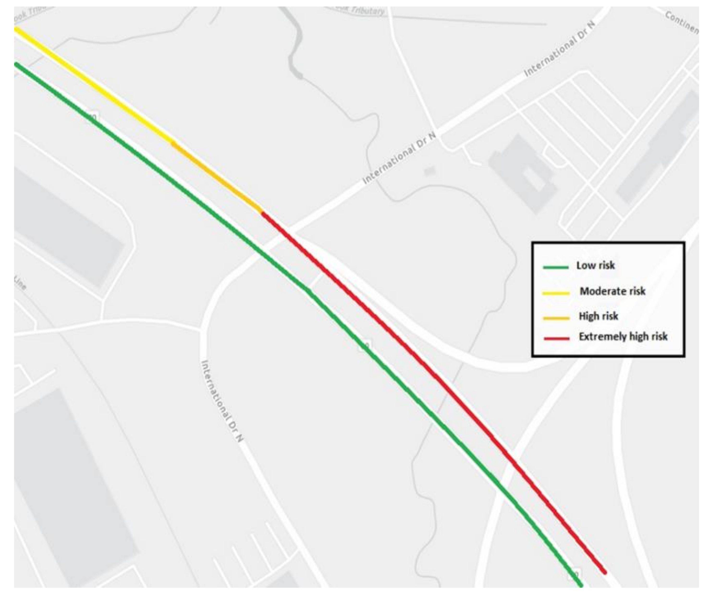
The outcomes of this research can be implemented in designing an operational traffic safety management system that can predict the relative short-term (e.g., next 5–15 min) crash risk for all regional roadways at the roadway segment level. For the operational purposes it is suggested to use relative crash likelihood as the measure of crash risk, instead of using the absolute crash probability values generated as model outputs. Each of the presented models calculates the probability of crash occurrence and its associated injury severity level for each road segment. These values can be clustered into multiple groups based on pre-defined thresholds that represent the relative risk of crash. To exemplify, the following values can be used to categorize the crash risk at a road segment level:

Low risk	if	Pi ≤ 0.3
Moderate risk	if	0.3 < Pi ≤ 0.6
High risk	if	0.6 < Pi ≤ 0.75
Extremely high risk	if	Pi > 0.75

To facilitate monitoring of the crash risk across a roadway network in real-time, a map-based system can be deployed in which the road segments are colored/labeled based on the associated relative crash risks (see a sample illustration in Figure 5). This is expected to help the traffic operations management authorities to take proactive traffic management strategies such as utilizing variable speed limits, variable message signs, and coordinated warning signals to mitigate crash risks at the high-risk locations.

8. Conclusions

The main goal of this study was to apply advanced data analytics methods to develop and evaluate crash prediction models that can be used in near-real-time. The application of several machine learning models for crash likelihood and crash severity prediction has been demonstrated in a case study of two interstate highways in New Jersey. The analysis dataset from which the explanatory variables and the response variables were derived included detailed crash data from the crash records database, basic roadway geometry data, synthetic vehicle volume and road segment capacity data, probe-vehicle traffic speed data, and weather data from the National Weather Service. In addition to crash records, the analysis included non-crash cases that were generated using the matched case-control methodology. To deal with the data imbalance between the non-injury (PDO) crashes and injury/fatal crashes, the study employed the random oversampling examples (ROSE) method. The relative importance of explanatory variables was evaluated using the RF model and they were ranked based on mean decrease accuracy (MDA).

The RBLR model further revealed (or rather confirmed) the significance of each explanatory variable in the crash prediction model. In addition to RBLR, the RF, GBM, GNB, and KNN models were also estimated for both crash likelihood and crash severity modeling. The predictive performance of the presented models was evaluated using the performance metrics that included overall accuracy, sensitivity, specificity, and the AUC value. The estimation results showed that the RF model outperformed all the other investigated models. However, none of the models based solely on the proactive data readily available to the transportation agencies performed sufficiently well for a meaningful and reliable application as operational models. The reason for such underperformance may be the lack of information and noise in the data used for model development. To address the potential shortcoming due to missing data features, a combined modeling framework has been presented that includes the data reflecting both proactive and reactive factors. The proposed method produced an improvement in the predictive performance of the injury severity model by incorporating the reactive data on driver age and vehicle age. This is achieved through implementation of a modeling framework that evaluates injury severities for different crash classes defined for different combinations of driver age and vehicle age.

It is postulated that the results of this study could help the transportation agencies and decision-makers in advancing the design and implementation of more effective operational decision support systems for roadway safety management. Such systems would assist the traffic operations personnel in implementation of operational countermeasures and tactics to reduce the likelihood of crashes, such as proactive activation of advanced warnings on variable message sign (VMS), adjustments of variable speed limits (VSL), ramp metering (RM), or deployment of highway patrol and law enforcement resources to roadway segments with higher crash risk. The proposed modeling framework also provide a basis for further research in crash risk prediction, considering the emerging datasets. Such datasets include driving behavior records collected by the vehicle telemetry and user-based insurance (UBI) systems, which are already being offered to the policy holders by the major insurance companies. Another possible source of useful data are naturalistic driving studies [38], which can also be incorporated in the analysis to achieve more accurate predictive models. Using this rich source of data will enable the prediction of crash likelihood and injury severity by simultaneous use of proactive data and reactive data, such as driver and vehicle characteristics. The increasing adoption of connected vehicle technology and the share of connected vehicles on the roads will also provide the opportunity to utilize vehicle telemetry and driver behavior data in near real time, which can further improve the performance of the crash risk prediction models proposed in this research.

The addition of the variables that have not been considered in this study such as the presence of a work zone and the locations of interchanges/intersections relative to the roadway segment, may be beneficial towards the improved accuracy and predictive capability of the ML models and may shed more light on potential pros and cons of including certain variables in the ML models. Along with consideration of connected vehicle and vehicle telemetry data, the addition of those factors and the corresponding parameters in the analysis is a promising future research direction.

References

- Darban Khales, S.; Kunt, M.M.; Dimitrijevic, B. Analysis of the impacts of risk factors on teenage and older driver injury severity using random-parameter ordered probit. Can. J. Civ. Eng. 2020, 47, 1249–1257. [Google Scholar] [CrossRef]
- Chen, C.; Zhang, G.; Yang, J.; Milton, J.C. An explanatory analysis of driver injury severity in rear-end crashes using a decision table/Naïve Bayes (DTNB) hybrid classifier. Accid. Anal. Prev. 2016, 90, 95–107. [Google Scholar] [CrossRef] [PubMed]
- Iranitalab, A.; Khattak, A. Comparison of four statistical and machine learning methods for crash severity prediction. Accid. Anal. Prev. 2017, 108, 27–36. [Google Scholar] [CrossRef] [PubMed]
- Reiman, T.; Pietikäinen, E. Leading indicators of system safety–monitoring and driving the organizational safety potential. Saf. Sci. 2012, 50, 1993–2000. [Google Scholar] [CrossRef]
- Sarkar, S.; Pramanik, A.; Maiti, J.; Reniers, G. Predicting and analyzing injury severity: A machine learning-based approach using class-imbalanced proactive and reactive data. Saf. Sci. 2020, 125, 104616. [Google Scholar] [CrossRef]
- Xu, C.; Tarko, A.P.; Wang, W.; Liu, P. Predicting crash likelihood and severity on freeways with real-time loop detector data. Accid. Anal. Prev. 2013, 57, 30–39. [Google Scholar] [CrossRef] [PubMed]
- Theofilatos, A. Incorporating real-time traffic and weather data to explore road accident likelihood and severity in urban arterials. J. Saf. Res. 2017, 61, 9–21. [Google Scholar] [CrossRef]
- Yu, R.; Abdel-Aty, M. Utilizing support vector machine in real-time crash risk evaluation. Accid. Anal. Prev. 2013, 51, 252–259. [Google Scholar] [CrossRef]
- Wang, L.; Shi, Q.; Abdel-Aty, M. Predicting crashes on expressway ramps with real-time traffic and weather data. Transp. Res. Rec. 2015, 2514, 32–38. [Google Scholar] [CrossRef]
- Theofilatos, A.; Chen, C.; Antoniou, C. Comparing machine learning and deep learning methods for real-time crash prediction. Transp. Res. Rec. 2019, 2673, 169–178. [Google Scholar] [CrossRef]
- Guo, M.; Zhao, X.; Yao, Y.; Yan, P.; Su, Y.; Bi, C.; Wu, D. A study of freeway crash risk prediction and interpretation based on risky driving behavior and traffic flow data. Accid. Anal. Prev. 2021, 160, 106328. [Google Scholar] [CrossRef] [PubMed]
- Wang, C.; Liu, L.; Xu, C.; Lv, W. Predicting future driving risk of crash-involved drivers based on a systematic machine learning framework. Int. J. Environ. Res. Public Health 2019, 16, 334. [Google Scholar] [CrossRef] [PubMed] [Green Version]
- Sameen, M.I.; Pradhan, B. Severity prediction of traffic accidents with recurrent neural networks. Appl. Sci. 2017, 7, 476. [Google Scholar] [CrossRef] [Green Version]
- Lin, C.; Wu, D.; Liu, H.; Xia, X.; Bhattarai, N. Factor identification and prediction for teen driver crash severity using machine learning: A case study. Appl. Sci. 2020, 10, 1675. [Google Scholar] [CrossRef] [Green Version]
- Zhang, J.; Li, Z.; Pu, Z.; Xu, C. Comparing prediction performance for crash injury severity among various machine learning and statistical methods. IEEE Access 2018, 6, 60079–60087. [Google Scholar] [CrossRef]
- Wahab, L.; Jiang, H. A comparative study on machine learning based algorithms for prediction of motorcycle crash severity. PLoS ONE 2019, 14, e0214966. [Google Scholar] [CrossRef]
- Kim, S.; Lym, Y.; Kim, K.-J. Developing crash severity model handling class imbalance and implementing ordered nature: Focusing on elderly drivers. Int. J. Environ. Res. Public Health 2021, 18, 1966. [Google Scholar] [CrossRef]
- Fiorentini, N.; Losa, M. Handling imbalanced data in road crash severity prediction by machine learning algorithms. Infrastructures 2020, 5, 61. [Google Scholar] [CrossRef]
- Breiman, L.; Friedman, J.H.; Olshen, R.A.; Stone, C.J. Classification and Regression Trees; Wadsworth and Brooks: Monterey, CA, USA, 1984. [Google Scholar]
- Breiman, L. Some Infinity Theory for Predictor Ensembles; Technical Report. Report No. 579; Statistics Department, University of California: Berkeley, CA, USA, 2000. [Google Scholar]
- Nicodemus, K.K. Letter to the editor: On the stability and ranking of predictors from random forest variable importance measures. Brief. Bioinform. 2011, 12, 369–373. [Google Scholar] [CrossRef] [Green Version]
- Bishop, C.M. Pattern Recognition and Machine Learning; Springer: Berlin, Germany, 2006. [Google Scholar]
- Cigdem, A.; Ozden, C. Predicting the severity of motor vehicle accident injuries in Adana-Turkey using machine learning methods and detailed meteorological data. Int. J. Intell. Syst. Appl. Eng. 2018, 6, 72–79. [Google Scholar]
- Shanthi, S.; Ramani, R.G. Classification of vehicle collision patterns in road accidents using data mining algorithms. Int. J. Comput. Appl. 2011, 35, 30–37. [Google Scholar]
- Stafford, B. Pysolar. 2021. Available online: https://media.readthedocs.org/pdf/pysolar/latest/pysolar.pdf (accessed on 8 November 2021).
- Li, X.; Cai, B.Y.; Qiu, W.; Zhao, J.; Ratti, C. A novel method for predicting and mapping the occurrence of sun glare using Google Street View. Transp. Res. Part C Emerg. Technol. 2019, 106, 132–144. [Google Scholar] [CrossRef]
- Ahmed, M.M.; Abdel-Aty, M.A. The viability of using automatic vehicle identification data for real-time crash prediction. IEEE Trans. Intell. Transp. Syst. 2011, 13, 459–468. [Google Scholar] [CrossRef]
- Menardi, G.; Torelli, N. Training and assessing classification rules with imbalanced data. Data Min. Knowl. Discov. 2014, 28, 92–122. [Google Scholar] [CrossRef]
- Tibshirani, R.J.; Efron, B. An Introduction to the Bootstrap. In Monographs on Statistics and Applied Probability; CRC Press: Boca Raton, FL, USA, 1993; Volume 57, pp. 1–436. [Google Scholar]
- Bowman, A.W.; Azzalini, A. Applied Smoothing Techniques for Data Analysis: The Kernel Approach with S-Plus Illustrations; Oxford University Press: Oxford, UK, 1997. [Google Scholar]
- Gelman, A. Objections to Bayesian statistics. Bayesian Anal. 2008, 3, 445–449. [Google Scholar] [CrossRef]
- Lunn, D.; Jackson, C.; Best, N.; Thomas, A.; Spiegelhalter, D. The BUGS Book: A Practical Introduction to Bayesian Analysis; CRC Press: Boca Raton, FL, USA, 2012. [Google Scholar]
- StataCorp, LLC. Stata Bayesian Analysis Reference Manual; StataCorp, LLC.: College Station, TX, USA, 2017. [Google Scholar]
- Kuhn, M.; Wing, J.; Weston, S.; Williams, A.; Keefer, C.; Engelhardt, A.; Cooper, T.; Mayer, Z.; Benesty, M.; Lescarbeau, R.; et al. Package ‘caret’. R J. 2020, 223, 7. [Google Scholar]
- Opitz, D.; Maclin, R. Popular ensemble methods: An empirical study. J. Artif. Intell. Res. 1999, 11, 169–198. [Google Scholar] [CrossRef]
- Hastie, T.; Tibshirani, R.; Friedman, J. The Elements of Statistical Learning: Data Mining, Inference, and Prediction; Springer: New York, NY, USA, 2009. [Google Scholar]
- Friedman, J.H. Greedy function approximation: A gradient boosting machine. Ann. Stat. 2001, 29, 1189–1232. [Google Scholar] [CrossRef]
- Dingus, T.A.; Klauer, S.G.; Neale, V.L.; Petersen, A.; Lee, S.E.; Sudweeks, J.; Perez, M.A.; Hankey, J.; Ramsey, D.; Gupta, S.; et al. The 100-Car Naturalistic Driving Study, Phase II-Results of the 100-Car Field Experiment; Department of Transportation, National Highway Traffic Safety Administration: Washington, DC, USA, 2006. [Google Scholar]