
Adaptive Neural Network Control of Zero-Speed Vessel Fin Stabilizer Based on Command Filter


Abstract
:1. Introduction
2. Problem Formulation and Preliminaries
2.1. Problem Formulation
2.2. Preliminaries
3. Controller Design and Stability Analysis
3.1. Control Law Design
3.2. Stability Analysis
- (1)
- The closed-loop control system is stable and all signals of the closed-loop control system are ultimately uniformly bounded;
- (2)
- When appropriate design parameters , , , , and L are selected, the error between the actual roll angle φ of the vessel roll control system and the expected roll angle can converge to a small residual set;
- (3)
- Under the influence of input saturation, the error satisfies:
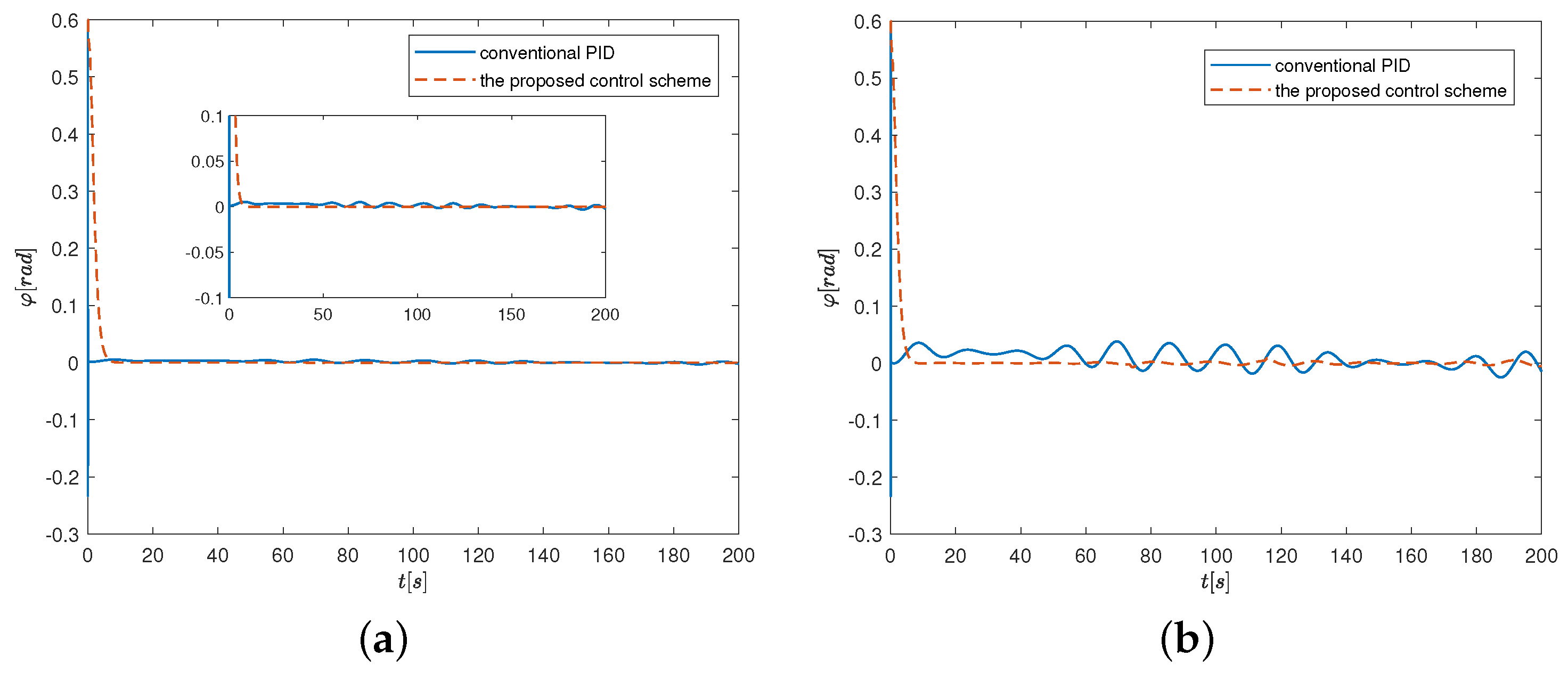
4. Simulation
5. Conclusions
Author Contributions
Funding
Institutional Review Board Statement
Informed Consent Statement
Data Availability Statement
Conflicts of Interest
Abbreviations
| ADS | Auxiliary dynamic system |
| RBF | Radial basis function |
| NN | Neural network |
| PID | Proportion integral differential |
| AES | Augmented error signal |
| ISS | Input-to-state stable |
References
- Li, R.; Li, T.; Bai, W.; Du, X. An adaptive neural network approach for ship roll stabilization via fin control. Neurocomputing 2016, 173, 953–957. [Google Scholar] [CrossRef]
- Baniela, S.I. Roll motion of a ship and the roll stabilising effect of bilge keels. J. Navig. 2008, 61, 667–686. [Google Scholar] [CrossRef]
- Zhao, J.; Liang, C.; Zhang, X. Rudder roll stabilization based on arc tangent nonlinear feedback for ships. J. Mar. Sci. Eng. 2020, 8, 245. [Google Scholar] [CrossRef] [Green Version]
- Subramanian, R.; Jyothish, P.V. Genetic algorithm based design optimization of a passive anti-roll tank in a sea going vessel. Ocean Eng. 2020, 203, 107216. [Google Scholar] [CrossRef]
- Luo, W.; Hu, B.; Li, T. Neural network based fin control for ship roll stabilization with guaranteed robustness. J. Abbr. 2017, 230, 210–218. [Google Scholar] [CrossRef]
- Jiguang, S.; Lihua, L.; Zhang, S.; Wang, J. Design and experimental investigation of a GA-based control strategy for a low-speed fin stabilizer. Ocean Eng. 2020, 218, 108234. [Google Scholar] [CrossRef]
- Alarçin, F.; Demirel, H.; Su, M.E.; Yurtseven, A. Modified pid control design for roll fin actuator of nonlinear modelling of the fishing boat. Pol. Marit. Res. 2014, 1, 3–8. [Google Scholar] [CrossRef] [Green Version]
- Liang, L.; Zhao, P.; Zhang, S.; Ji, M.; Song, J.; Yuan, J. Simulation and experimental study on control strategy of zero-speed fin stabilizer based on disturbance and compensation. PLoS ONE 2018, 13, e0204446. [Google Scholar] [CrossRef]
- Hickey, N.A.; Grimble, M.J.; Johnson, M.A.; Katebi, M.R.; Melville, R. Robust fin roll stabilisation of surface ships. In Proceedings of the 36th IEEE Conference on Decision and Control, San Diego, CA, USA, 12 December 1997; Volume 5, pp. 4225–4230. [Google Scholar]
- Koshkouei, A.J.; Law, Y.; Burnham, K.J. Sliding mode and PID controllers for ship roll stabilisation: A comparative simulation study. IFAC Proc. Vol. 2005, 38, 7–12. [Google Scholar] [CrossRef] [Green Version]
- Jin, Z.; Zhang, W.; Liu, S.; Gu, M. Command-filtered backstepping integral sliding mode control with prescribed performance for ship roll stabilization. Appl. Sci. 2019, 9, 4288. [Google Scholar] [CrossRef] [Green Version]
- Perez, T.; Goodwin, G.C. Constrained predictive control of ship fin stabilizers to prevent dynamic stall. Control Eng. Pract. 2008, 16, 482–494. [Google Scholar] [CrossRef]
- Karakas, S.; Ucer, E.; Pesman, E. Control design of fin roll stabilization in beam seas based on Lyapunov’s direct method. Pol. Marit. Res. 2012, 19, 25–30. [Google Scholar] [CrossRef] [Green Version]
- Xu, H.; Oliveira, P.; Soares, C.G. L1 adaptive backstepping control for path-following of underactuated marine surface ships. Eur. J. Control 2021, 58, 357–372. [Google Scholar] [CrossRef]
- Yang, Y.; Zhou, C.; Jia, X. Robust adaptive fuzzy control and its application to ship roll stabilization. Inf. Sci. 2002, 142, 177–194. [Google Scholar] [CrossRef]
- Yang, Y.; Jiang, B. Variable structure robust fin control for ship roll stabilization with actuator system. In Proceedings of the 2004 American Control Conference, Boston, MA, USA, 30 June–2 July 2004; Volume 6, pp. 5212–5217. [Google Scholar]
- Bai, W.; Li, T.; Li, R. Neural network based direct adaptive for fin stabilizer system with input saturation. Mar. Eng. Front. 2013, 1, 63–68. [Google Scholar]
- Sun, M.; Luan, T.; Liang, L. RBF neural network compensation-based adaptive control for lift-feedback system of ship fin stabilizers to improve anti-rolling effect. Ocean Eng. 2018, 163, 307–321. [Google Scholar] [CrossRef]
- Ping, Y.U. Study of fin stabilizer’s control system based on neural network for nonlinear roll motion of ship. Inf. Control 2003, 3, 264–267. [Google Scholar]
- Hui, L.; Chen, G.; Jin, H. Design of adaptive inverse mode wavelet neural network controller of fin stabilizer. Int. Conf. Neural Netw. Brain 2005, 3, 1745–1748. [Google Scholar]
- Zhang, Y.T.; Shi, W.R.; Qiu, M.B. Sliding backstepping control for fin stabilizer with nonlinear disturbance observer. Control Decis. 2010, 25, 1255–1260. [Google Scholar]
- Liang, L.; Wen, Y. Disturbance compensation model predictive control for integrated rudder/fin roll stabilization. In Proceedings of the 2018 37th Chinese Control Conference (CCC), Wuhan, China, 25–27 July 2018; pp. 3859–3864. [Google Scholar]
- Gong, S.; Song, L.; Tian, Y. PID control to rudder roll damping based on disturbance observer. Mar. Electr. Electron. Eng. 2005, 33, 23–26. [Google Scholar]
- Han, Y. Neural disturbance observer based sliding mode control and its application to yaw/roll joint stabilization. J. Comput. Inf. Syst. 2014, 10, 7399–7406. [Google Scholar]
- Chen, W.-H. Disturbance observer based control for nonlinear systems. IEEE/ASME Trans. Mechatron. 2004, 9, 706–710. [Google Scholar] [CrossRef] [Green Version]
- Wu, J.; Huang, J.; Wang, Y.; Xing, K. Nonlinear disturbance observer-based dynamic surface control for trajectory tracking of pneumatic muscle system. IEEE Trans. Control Syst. Technol. 2013, 22, 440–455. [Google Scholar] [CrossRef]
- Yang, J.; Li, S.; Yu, X. Sliding-mode control for systems with mismatched uncertainties via a disturbance observer. IEEE Trans. Ind. Electron. 2012, 60, 160–169. [Google Scholar] [CrossRef]
- Lihua, L.; Peng, Z.; Songtao, Z.; Jia, Y. Simulation analysis of fin stabilizers on turning circle control during ship turns. Ocean Eng. 2019, 173, 174–182. [Google Scholar] [CrossRef]
- Shao, K.; Tang, R.; Xu, F.; Wang, X.; Zheng, J. Adaptive sliding mode control for uncertain Euler–Lagrange systems with input saturation. J. Frankl. Inst. 2021, 358, 8356–8376. [Google Scholar] [CrossRef]
- Lauvdal, T.; Fossen, T.I. Rudder roll stabilization of ships subject to input rate saturation using a gain scheduled control law. IFAC Proc. Vol. 1998, 30, 111–116. [Google Scholar] [CrossRef]
- Ge, D.; Gao, Q.; Li, A.; Chen, Y. Rudder roll stabilization for ships with generalized predictive control based on fuzzy gain scheduler. In Proceedings of the 2009 IEEE International Conference on Intelligent Computing and Intelligent Systems, Shanghai, China, 20–22 November 2009; Volume 2, pp. 426–429. [Google Scholar]
- Esmailian, E.; Farzanegan, B.; Menhaj, M.B.; Ghassemi, H. A robust neuro-based adaptive control system design for a surface effect ship with uncertain dynamics and input saturation to cargo transfer at sea. Appl. Ocean. Res. 2018, 74, 59–68. [Google Scholar] [CrossRef]
- Zheng, Z.; Huang, Y.; Xie, L.; Zhu, B. Adaptive trajectory tracking control of a fully actuated surface vessel with asymmetrically constrained input and output. IEEE Trans. Control. Syst. Technol. 2017, 26, 1851–1859. [Google Scholar] [CrossRef]
- Zhu, G.; Ma, Y.; Li, Z.; Malekian, R.; Sotelo, M. Event-triggered adaptive neural fault-tolerant control of underactuated msvs with input saturation. IEEE Trans. Intell. Transp. Syst. 2021, 1–13. [Google Scholar] [CrossRef]
- Zhu, G.; Du, J.; Kao, Y. Command filtered robust adaptive NN control for a class of uncertain strict-feedback nonlinear systems under input saturation. J. Frankl. Inst. 2018, 355, 7548–7569. [Google Scholar] [CrossRef]
- Bai, W.; Li, T.; Gao, X.; Myint, K.T. Neural network based direct adaptive backstepping method for fin stabilizer system. In International Symposium on Neural Networks; Springer: Berlin/Heidelberg, Germany, 2013; pp. 212–219. [Google Scholar]
- Wen, C.; Zhou, J.; Liu, Z.; Su, H. Robust adaptive control of uncertain nonlinear systems in the presence of input saturation and external disturbance. IEEE Trans. Autom. Control 2011, 56, 1672–1678. [Google Scholar] [CrossRef]
- Zhou, J.; Wen, C. Robust adaptive control of uncertain nonlinear systems in the presence of input saturation. IFAC Proc. Vol. 2006, 39, 149–154. [Google Scholar] [CrossRef]
- Liu, Q.; Li, D.; Ge, S.S.; Ji, R.; Ouyang, Z.; Tee, K.P. Adaptive bias RBF neural network control for a robotic manipulator. Neurocomputing 2021, 447, 213–223. [Google Scholar] [CrossRef]
- Liu, S.; Liu, Y.; Wang, N. Nonlinear disturbance observer-based backstepping finite-time sliding mode tracking control of underwater vehicles with system uncertainties and external disturbances. Nonlinear Dyn. 2017, 88, 465–476. [Google Scholar] [CrossRef]
- Farrell, J.A.; Polycarpou, M.; Sharma, M.; Dong, W. Command filtered backstepping. IEEE Trans. Autom. Control 2009, 54, 1391–1395. [Google Scholar] [CrossRef]


Publisher’s Note: MDPI stays neutral with regard to jurisdictional claims in published maps and institutional affiliations. |
© 2022 by the authors. Licensee MDPI, Basel, Switzerland. This article is an open access article distributed under the terms and conditions of the Creative Commons Attribution (CC BY) license (https://creativecommons.org/licenses/by/4.0/).
Share and Cite
Sun, Z.; Chen, C.; Zhu, G. Adaptive Neural Network Control of Zero-Speed Vessel Fin Stabilizer Based on Command Filter. Appl. Sci. 2022, 12, 754. https://doi.org/10.3390/app12020754
Sun Z, Chen C, Zhu G. Adaptive Neural Network Control of Zero-Speed Vessel Fin Stabilizer Based on Command Filter. Applied Sciences. 2022; 12(2):754. https://doi.org/10.3390/app12020754
Chicago/Turabian StyleSun, Ziteng, Chao Chen, and Guibing Zhu. 2022. "Adaptive Neural Network Control of Zero-Speed Vessel Fin Stabilizer Based on Command Filter" Applied Sciences 12, no. 2: 754. https://doi.org/10.3390/app12020754