
Automated Recognition of Chemical Molecule Images Based on an Improved TNT Model


Abstract
:1. Introduction
2. Related Work
2.1. Image Captioning
2.2. Transformer
3. Materials and Methods
3.1. Transformer
3.2. Vision Transformer
3.3. Deep-TNT Block
3.4. Position Encoding
3.5. Parameter Setting in the Network Architecture
4. Results
4.1. Setup
4.1.1. Datasets
4.1.2. Models for Comparison
4.1.3. Pre-Processing
4.1.4. Training Details
4.2. Comparison
4.3. Ablation
4.4. Analysis of Inference Results
4.5. Inference & Fusion
5. Conclusions
Author Contributions
Funding
Institutional Review Board Statement
Informed Consent Statement
Data Availability Statement
Conflicts of Interest
References
- BMS-Molecular-Translation. 2021. Available online: https://www.kaggle.com/c/bms-molecular-translation (accessed on 1 November 2021).
- LeCun, Y.; Boser, B.; Denker, J.S.; Henderson, D.; Howard, R.E.; Hubbard, W.; Jackel, L.D. Backpropagation Applied to Handwritten Zip Code Recognition. Neural Comput. 1989, 1, 541–551. [Google Scholar] [CrossRef]
- Krizhevsky, A.; Sutskever, I.; Hinton, G.E. ImageNet Classification with Deep Convolutional Neural Networks. Adv. Neural Inf. Process. Syst. 2012, 25, 1097–1105. [Google Scholar] [CrossRef]
- He, K.; Zhang, X.; Ren, S.; Sun, J. Deep Residual Learning for Image Recognition. In Proceedings of the IEEE Conference on Computer Vision and Pattern Recognition, Las Vegas, NV, USA, 27–30 June 2016; pp. 770–778. [Google Scholar]
- Tan, M.; Le, Q. Efficientnet: Rethinking Model Scaling for Convolutional Neural Networks. In Proceedings of the International Conference on Machine Learning, PMLR, Long Beach, CA, USA, 9–15 June 2019; pp. 6105–6114. [Google Scholar]
- Wang, C.; Yang, H.; Bartz, C.; Meinel, C. Image Captioning with Deep Bidirectional LSTMs. In Proceedings of the 24th ACM International Conference on Multimedia, Amsterdam, The Netherlands, 15–19 October 2016; pp. 988–997. [Google Scholar]
- Vaswani, A.; Shazeer, N.; Parmar, N.; Uszkoreit, J.; Jones, L.; Gomez, A.N.; Kaiser, Ł.; Polosukhin, I. Attention Is All You Need. In Proceedings of the 31st Conference on Neural Information Processing Systems (NeurIPS), Long Beach, CA, USA, 4–9 December 2017; pp. 5998–6008. [Google Scholar]
- Devlin, J.; Chang, M.W.; Lee, K.; Toutanova, K. BERT: Pre-training of Deep Bidirectional Transformers for Language Understanding. In Proceedings of the 2019 Conference of the North American Chapter of the Association for Computational Linguistics: Human Language Technologies, Volume 1 (Long and Short Papers), Minneapolis, MN, USA, 2–7 June 2019; pp. 4171–4186. [Google Scholar]
- Brown, T.B.; Mann, B.; Ryder, N.; Subbiah, M.; Kaplan, J.; Dhariwal, P.; Neelakantan, A.; Shyam, P.; Sastry, G.; Askell, A.; et al. Language Models are Few-Shot Learners. arXiv 2020, arXiv:2005.14165. [Google Scholar]
- Dosovitskiy, A.; Beyer, L.; Kolesnikov, A.; Weissenborn, D.; Zhai, X.; Unterthiner, T.; Dehghani, M.; Minderer, M.; Heigold, G.; Gelly, S.; et al. An Image is Worth 16 × 16 Words: Transformers for Image Recognition at Scale. In Proceedings of the International Conference on Learning Representations, Addis Ababa, Ethiopia, 26–30 April 2020. [Google Scholar]
- Touvron, H.; Cord, M.; Douze, M.; Massa, F.; Sablayrolles, A.; Jégou, H. Training Data-Efficient Image Transformers & Distillation through Attention. In Proceedings of the International Conference on Machine Learning, PMLR, Virtual, 18–24 July 2021; pp. 10347–10357. [Google Scholar]
- Han, K.; Xiao, A.; Wu, E.; Guo, J.; Xu, C.; Wang, Y. Transformer in Transformer. arXiv 2021, arXiv:2103.00112. [Google Scholar]
- Liu, Z.; Lin, Y.; Cao, Y.; Hu, H.; Wei, Y.; Zhang, Z.; Lin, S.; Guo, B. Swin Transformer: Hierarchical Vision Transformer using Shifted Windows. arXiv 2021, arXiv:2103.14030. [Google Scholar]
- Frome, A.; Corrado, G.S.; Shlens, J.; Bengio, S.; Dean, J.; Ranzato, M.; Mikolov, T. DeViSE: A Deep Visual-Semantic Embedding Model. Adv. Neural Inf. Process. Syst. 2013, 26, 2121–2129. [Google Scholar]
- Mori, Y.; Takahashi, H.; Oka, R. Image-To-Word Transformation Based on Dividing and Vector Quantizing Images with Words. In Proceedings of the MISRM’99 First International Workshop on Multimedia Intelligent Storage and Retrieval Management, Orlando, FL, USA, 30 October 1999. [Google Scholar]
- Kuznetsova, P.; Ordonez, V.; Berg, A.; Berg, T.; Choi, Y. Collective Generation of Natural Image Descriptions. In Proceedings of the 50th Annual Meeting of the Association for Computational Linguistics (Volume 1: Long Papers), Jeju Island, Korea, 8–14 July 2012; pp. 359–368. [Google Scholar]
- Elliott, D.; Keller, F. Image Description using Visual Dependency Representations. In Proceedings of the 2013 Conference on Empirical Methods in Natural Language Processing, Seattle, WA, USA, 18–21 October 2013; pp. 1292–1302. [Google Scholar]
- Ordonez, V.; Kulkarni, G.; Berg, T. Im2Text: Describing Images Using 1 Million Captioned Photographs. Adv. Neural Inf. Process. Syst. 2011, 24, 1143–1151. [Google Scholar]
- Felzenszwalb, P.F.; Girshick, R.B.; McAllester, D.; Ramanan, D. Object Detection with Discriminatively Trained Part-Based Models. IEEE Trans. Pattern Anal. Mach. Intell. 2009, 32, 1627–1645. [Google Scholar] [CrossRef] [PubMed] [Green Version]
- Mason, R.; Charniak, E. Nonparametric Method for Data-Driven Image Captioning. In Proceedings of the 52nd Annual Meeting of the Association for Computational Linguistics (Volume 2: Short Papers), Baltimore, MD, USA, 22–27 June 2014; pp. 592–598. [Google Scholar]
- Mao, J.; Xu, W.; Yang, Y.; Wang, J.; Yuille, A.L. Deep Captioning with Multimodal Recurrent Neural Networks (m-RNN). In Proceedings of the ICLR ’15 3rd International Conference on Learning Representations, San Diego, CA, USA, 7–9 May 2015. [Google Scholar]
- Vinyals, O.; Toshev, A.; Bengio, S.; Erhan, D. Show And Tell: A Neural Image Caption Generator. In Proceedings of the IEEE Conference on Computer Vision and Pattern Recognition, Boston, MA, USA, 7–12 June 2015; pp. 3156–3164. [Google Scholar]
- Mao, J.; Huang, J.; Toshev, A.; Camburu, O.; Yuille, A.L.; Murphy, K. Generation and Comprehension of Unambiguous Object Descriptions. In Proceedings of the IEEE Conference on Computer Vision and Pattern Recognition, Las Vegas, NV, USA, 27–30 June 2016; pp. 11–20. [Google Scholar]
- Xu, K.; Ba, J.; Kiros, R.; Cho, K.; Courville, A.; Salakhudinov, R.; Zemel, R.; Bengio, Y. Show, Attend and Tell: Neural Image Caption Generation with Visual Attention. In Proceedings of the International Conference on Machine Learning, PMLR, Lille, France, 7–9 July 2015; pp. 2048–2057. [Google Scholar]
- Anderson, P.; He, X.; Buehler, C.; Teney, D.; Johnson, M.; Gould, S.; Zhang, L. Bottom-Up and Top-Down Attention for Image Captioning and Visual Question Answering. In Proceedings of the IEEE Conference on Computer Vision and Pattern Recognition, Salt Lake City, UT, USA, 18–23 June 2018; pp. 6077–6086. [Google Scholar]
- Ye, S.; Han, J.; Liu, N. Attentive Linear Transformation for Image Captioning. IEEE Trans. Image Process. 2018, 27, 5514–5524. [Google Scholar] [CrossRef] [PubMed]
- Lu, J.; Yang, J.; Batra, D.; Parikh, D. Neural Baby Talk. In Proceedings of the IEEE Conference on Computer Vision and Pattern Recognition, Salt Lake City, UT, USA, 18–23 June 2018; pp. 7219–7228. [Google Scholar]
- Guo, L.; Liu, J.; Zhu, X.; Yao, P.; Lu, S.; Lu, H. Normalized and Geometry-Aware Self-Attention Network for Image Captioning. In Proceedings of the IEEE/CVF Conference on Computer Vision and Pattern Recognition, Seattle, WA, USA, 13–19 June 2020; pp. 10327–10336. [Google Scholar]
- Cornia, M.; Stefanini, M.; Baraldi, L.; Cucchiara, R. Meshed-Memory Transformer for Image Captioning. In Proceedings of the IEEE/CVF Conference on Computer Vision and Pattern Recognition, Seattle, WA, USA, 13–19 June 2020; pp. 10578–10587. [Google Scholar]
- Luo, Y.; Ji, J.; Sun, X.; Cao, L.; Wu, Y.; Huang, F.; Lin, C.W.; Ji, R. Dual-Level Collaborative Transformer for Image Captioning. In Proceedings of the AAAI Conference on Artificial Intelligence, New York, NY, USA, 2–9 February 2021; Volume 35, pp. 2286–2293. [Google Scholar]
- Li, L.H.; Yatskar, M.; Yin, D.; Hsieh, C.J.; Chang, K.W. VisualBERT: A Simple and Performant Baseline for Vision and Language. arXiv 2019, arXiv:1908.03557. [Google Scholar]
- Li, G.; Duan, N.; Fang, Y.; Gong, M.; Jiang, D. Unicoder-VL: A Universal Encoder for Vision and Language by Cross-Modal Pre-training. In Proceedings of the AAAI Conference on Artificial Intelligence, New York, NY, USA, 2–9 February 2020; Volume 34, pp. 11336–11344. [Google Scholar]
- Su, W.; Zhu, X.; Cao, Y.; Li, B.; Lu, L.; Wei, F.; Dai, J. VL-BERT: Pre-training of Generic Visual-Linguistic Representations. arXiv 2020, arXiv:1908.08530. [Google Scholar]
- Chen, Y.C.; Li, L.; Yu, L.; El Kholy, A.; Ahmed, F.; Gan, Z.; Cheng, Y.; Liu, J. UNITER: UNiversal Image-TExt Representation Learning. In Proceedings of the European Conference on Computer Vision, 16th European Conference, Glasgow, UK, 23–28 August 2020; Springer: Berlin/Heidelberg, Germany, 2020; pp. 104–120. [Google Scholar]
- Zhou, L.; Palangi, H.; Zhang, L.; Hu, H.; Corso, J.; Gao, J. Unified Vision-Language Pre-Training for Image Captioning and VQA. In Proceedings of the AAAI Conference on Artificial Intelligence, New York, NY, USA, 2–9 February 2020; Volume 34, pp. 13041–13049. [Google Scholar]
- Lu, J.; Batra, D.; Parikh, D.; Lee, S. ViLBERT: Pretraining Task-Agnostic Visiolinguistic Representations for Vision-and-Language Tasks. arXiv 2019, arXiv:1908.02265. [Google Scholar]
- Tan, H.; Bansal, M. LXMERT: Learning Cross-Modality Encoder Representations from Transformers; Inui, K., Jiang, J., Ng, V., Wan, X., Eds.; EMNLP/IJCNLP (1); Association for Computational Linguistics: Stroudsburg, PA, USA, 2019; pp. 5099–5110. [Google Scholar]
- Hu, J.; Shen, L.; Sun, G. Squeeze-and-Excitation Networks. In Proceedings of the IEEE Conference on Computer Vision and Pattern Recognition, Salt Lake City, UT, USA, 18–23 June 2018; pp. 7132–7141. [Google Scholar]
- Li, X.; Wang, W.; Hu, X.; Yang, J. Selective Kernel Networks. In Proceedings of the IEEE/CVF Conference on Computer Vision and Pattern Recognition, Long Beach, CA, USA, 18–20 June 2019; pp. 510–519. [Google Scholar]
- Zhang, H.; Wu, C.; Zhang, Z.; Zhu, Y.; Zhang, Z.; Lin, H.; Sun, Y.; He, T.; Mueller, J.; Manmatha, R.; et al. ResNeSt: Split-Attention Networks. arXiv 2020, arXiv:2004.08955. [Google Scholar]
- Wang, X.; Girshick, R.; Gupta, A.; He, K. Non-Local Neural Networks. In Proceedings of the IEEE Conference on Computer Vision and Pattern Recognition, Salt Lake City, UT, USA, 18–23 June 2018; pp. 7794–7803. [Google Scholar]
- Yin, M.; Yao, Z.; Cao, Y.; Li, X.; Zhang, Z.; Lin, S.; Hu, H. Disentangled Non-Local Neural Networks. In Proceedings of the European Conference on Computer Vision, 16th European Conference, Glasgow, UK, 23–28 August 2020; Springer: Berlin/Heidelberg, Germany, 2020; pp. 191–207. [Google Scholar]
- Yuan, Y.; Huang, L.; Guo, J.; Zhang, C.; Chen, X.; Wang, J. OCNet: Object Context Network for Scene Parsing. arXiv 2018, arXiv:1809.00916. [Google Scholar]
- Hu, H.; Gu, J.; Zhang, Z.; Dai, J.; Wei, Y. Relation Networks for Object Detection. In Proceedings of the IEEE Conference on Computer Vision and Pattern Recognition, Salt Lake City, UT, USA, 18–23 June 2018; pp. 3588–3597. [Google Scholar]
- Beal, J.; Kim, E.; Tzeng, E.; Park, D.H.; Zhai, A.; Kislyuk, D. Toward Transformer-Based Object Detection. arXiv 2020, arXiv:2012.09958. [Google Scholar]
- Zhu, X.; Su, W.; Lu, L.; Li, B.; Wang, X.; Dai, J. Deformable DETR: Deformable Transformers for End-to-End Object Detection. arXiv 2020, arXiv:2010.04159. [Google Scholar]
- Carion, N.; Massa, F.; Synnaeve, G.; Usunier, N.; Kirillov, A.; Zagoruyko, S. End-to-End Object Detection with Transformers. In Proceedings of the European Conference on Computer Vision, 16th European Conference, Glasgow, UK, 23–28 August 2020; Springer: Berlin/Heidelberg, Germany, 2020; pp. 213–229. [Google Scholar]
- Zheng, S.; Lu, J.; Zhao, H.; Zhu, X.; Luo, Z.; Wang, Y.; Fu, Y.; Feng, J.; Xiang, T.; Torr, P.H.; et al. Rethinking Semantic Segmentation from a Sequence-to-Sequence Perspective with Transformers. In Proceedings of the IEEE/CVF Conference on Computer Vision and Pattern Recognition, Nashville, TN, USA, 19–25 June 2021; pp. 6881–6890. [Google Scholar]
- Chen, H.; Wang, Y.; Guo, T.; Xu, C.; Deng, Y.; Liu, Z.; Ma, S.; Xu, C.; Xu, C.; Gao, W. Pre-Trained Image Processing Transformer. In Proceedings of the IEEE/CVF Conference on Computer Vision and Pattern Recognition, Nashville, TN, USA, 19–25 June 2021; pp. 12299–12310. [Google Scholar]
- Hendrycks, D.; Gimpel, K. Gaussian Error Linear Units (GELUs). arXiv 2016, arXiv:1606.08415. [Google Scholar]
- Gehring, J.; Auli, M.; Grangier, D.; Yarats, D.; Dauphin, Y.N. Convolutional Sequence to Sequence Learning. In Proceedings of the International Conference on Machine Learning, PMLR, Sydney, Australia, 6–11 August 2017; pp. 1243–1252. [Google Scholar]
- Albumentations. 2021. Available online: https://github.com/albumentations-team/albumentations (accessed on 1 November 2021).
- Zhang, M.R.; Lucas, J.; Ba, J.; Hinton, G.E. Lookahead Optimizer: k steps forward, 1 step back. In Proceedings of the 33rd Conference on Neural Information Processing Systems (NeurIPS 2019), Vancouver, BC, Canada, 8–14 December 2019; pp. 9593–9604. [Google Scholar]
- Liu, L.; Jiang, H.; He, P.; Chen, W.; Liu, X.; Gao, J.; Han, J. On the Variance of the Adaptive Learning Rate and Beyond. arXiv 2019, arXiv:1908.03265. [Google Scholar]
- Raunak, V.; Dalmia, S.; Gupta, V.; Metze, F. On Long-Tailed Phenomena in Neural Machine Translation. In Proceedings of the EMNLP (Findings), Association for Computational Linguistics, Online, 16–20 November 2020; pp. 3088–3095. [Google Scholar]
- Lin, T.Y.; Goyal, P.; Girshick, R.; He, K.; Dollár, P. Focal Loss for Dense Object Detection. In Proceedings of the IEEE International Conference on Computer Vision, Venice, Italy, 22–29 October 2017; pp. 2980–2988. [Google Scholar]
- Szegedy, C.; Vanhoucke, V.; Ioffe, S.; Shlens, J.; Wojna, Z. Rethinking the Inception Architecture for Computer Vision. In Proceedings of the IEEE Conference on Computer Vision and Pattern Recognition, Las Vegas, NV, USA, 27–30 June 2016; pp. 2818–2826. [Google Scholar]
- Touvron, H.; Vedaldi, A.; Douze, M.; Jegou, H. Fixing the Train-Test Resolution Discrepancy. Adv. Neural Inf. Process. Syst. 2019, 32, 8252–8262. [Google Scholar]
- RDKit. 2021. Available online: https://github.com/rdkit/rdkit (accessed on 1 November 2021).
- Goyal, P.; Dollár, P.; Girshick, R.; Noordhuis, P.; Wesolowski, L.; Kyrola, A.; Tulloch, A.; Jia, Y.; He, K. Accurate, Large Minibatch SGD: Training ImageNet in 1 Hour. arXiv 2017, arXiv:1706.02677. [Google Scholar]


| Encoder | ||||||
|---|---|---|---|---|---|---|
| Dim # | Heads | Pixel/batch size | Depth | Hidden_size | Mlp_act | |
| Internal transformer block | 160 | 4 | 4 | 12 | 640 | GELU |
| Middle transformer block | 10 | 6 | 16 | 128 | GELU | |
| Exterior transformer block | 2560 | 10 | 32 | 5120 | GELU | |
| Decoder | ||||||
| Decoder dim | Heads | FFN dim | Depth | Vocab_size | text_dim | |
| Transformer-decoder | 2560 | 8 | 1024 | 3 | 193 | 384 |
| Pre-Processing | Optimizer | Batch Size | Learning Rate | Label Smooth | Loss Function | Data Augmentation |
|---|---|---|---|---|---|---|
| Image denoising | Lookahead ( = 0.5, k = 5) | 16 | 1e-4 | Anti-Focal loss ( = 0.5) | GaussNoise | |
| Smart cropping | RAdam ( = 0.9, = 0.99) | 32 | 2e-4 | / | / | RandomRotate90 |
| Padding resizing | / | 64+ | (4e-4)+ | / | / | PepperNoise (SNR = 0.996) |
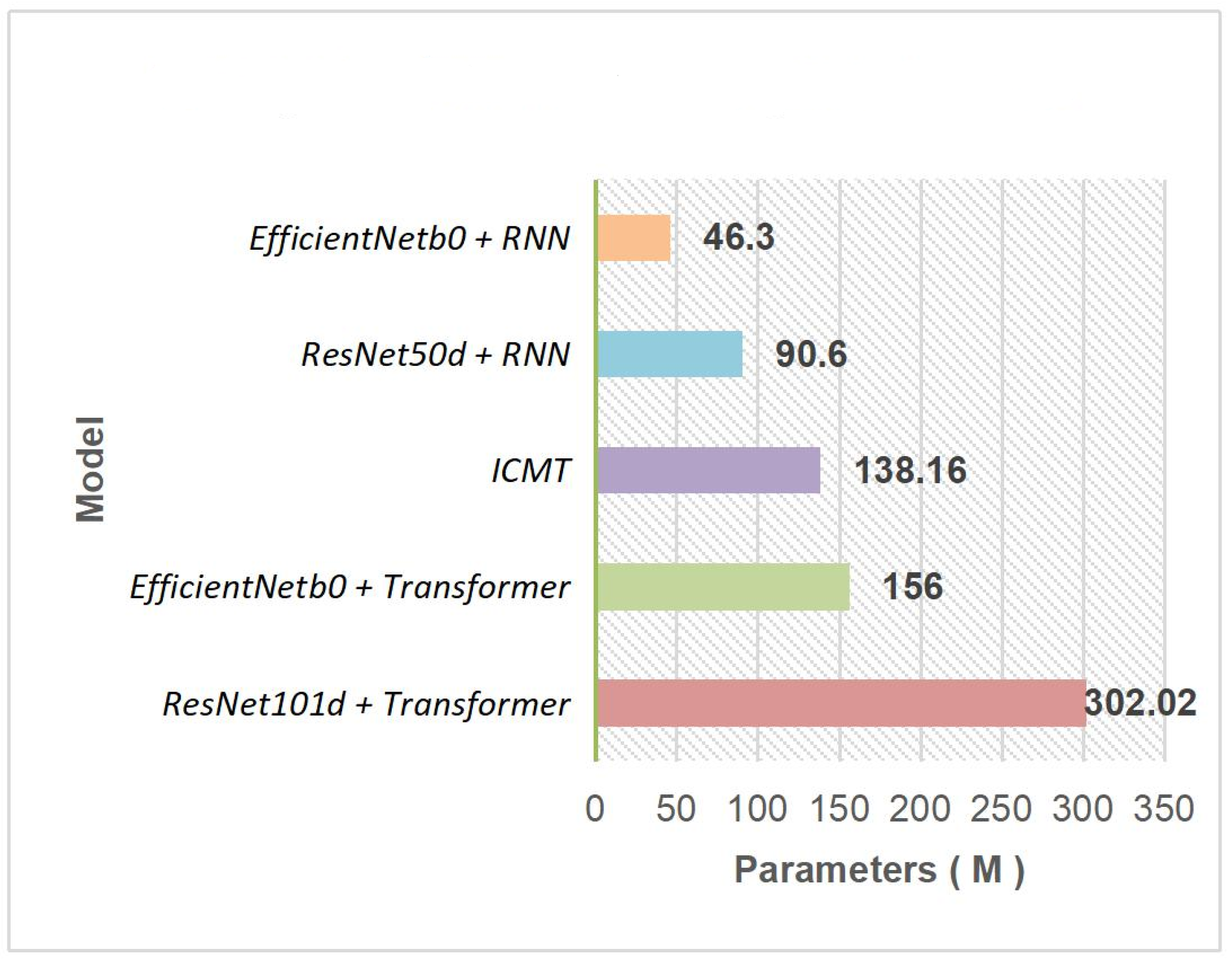
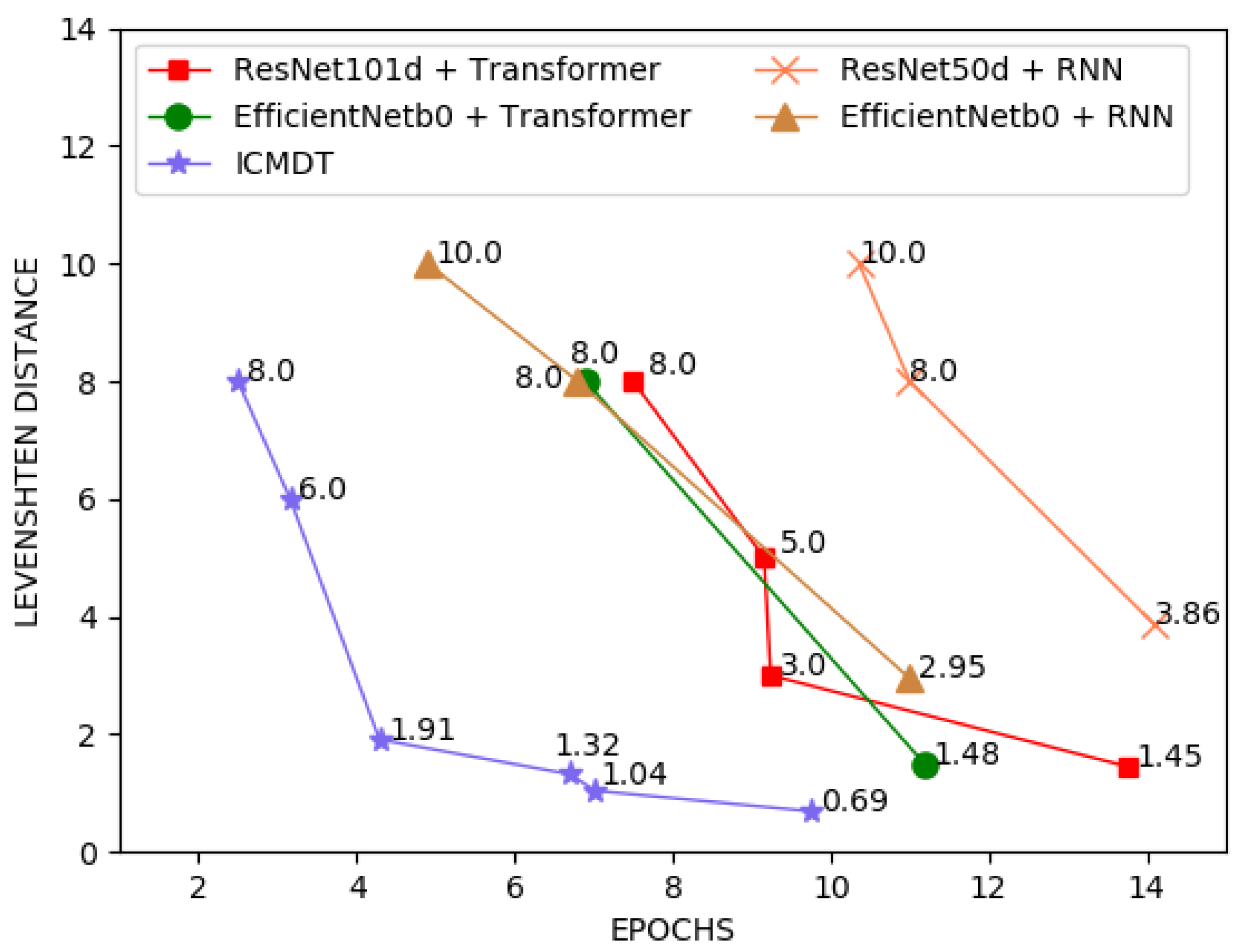
| Model | Parameters (M) | Levenshtein Distance |
|---|---|---|
| ICMDT | 138.16 | 0.69 |
| TNTD | 114.36 | 1.29 |
| TNTD-B | 114.36 | 1.37 |
| ICMDT* | 138.16 | 1.04 |
| Pre-Processing Strategy | Training Data Denoising | Smart Cropping | Padding Resizing | Test Data Denoising | Levenshtein Distance |
|---|---|---|---|---|---|
| Group 1 | √ | × | × | × | 7.69 |
| Group 2 | √ | × | × | √ | 2.69 |
| Group 3 | √ | √ | √ | × | 7.82 |
| Group 4 | √ | √ | √ | √ | 3.02 |
| Group 5 | √ | × | √ | × | 7.69 |
| Group 6 | √ | × | √ | √ | 2.69 |
| Denoised Training Data + Original Training Data | ||||||
|---|---|---|---|---|---|---|
| Proportion | 13:2 | 11:4 | 8:7 | 7:8 | 4:11 | 2:13 |
| Denoised test data | 7.5 | 6.32 | 5.02 | 5.0 | 2.69 | 1.04 |
| Original test data | 2.57 | 1.87 | 2.54 | 2.56 | 4.87 | 6.64 |
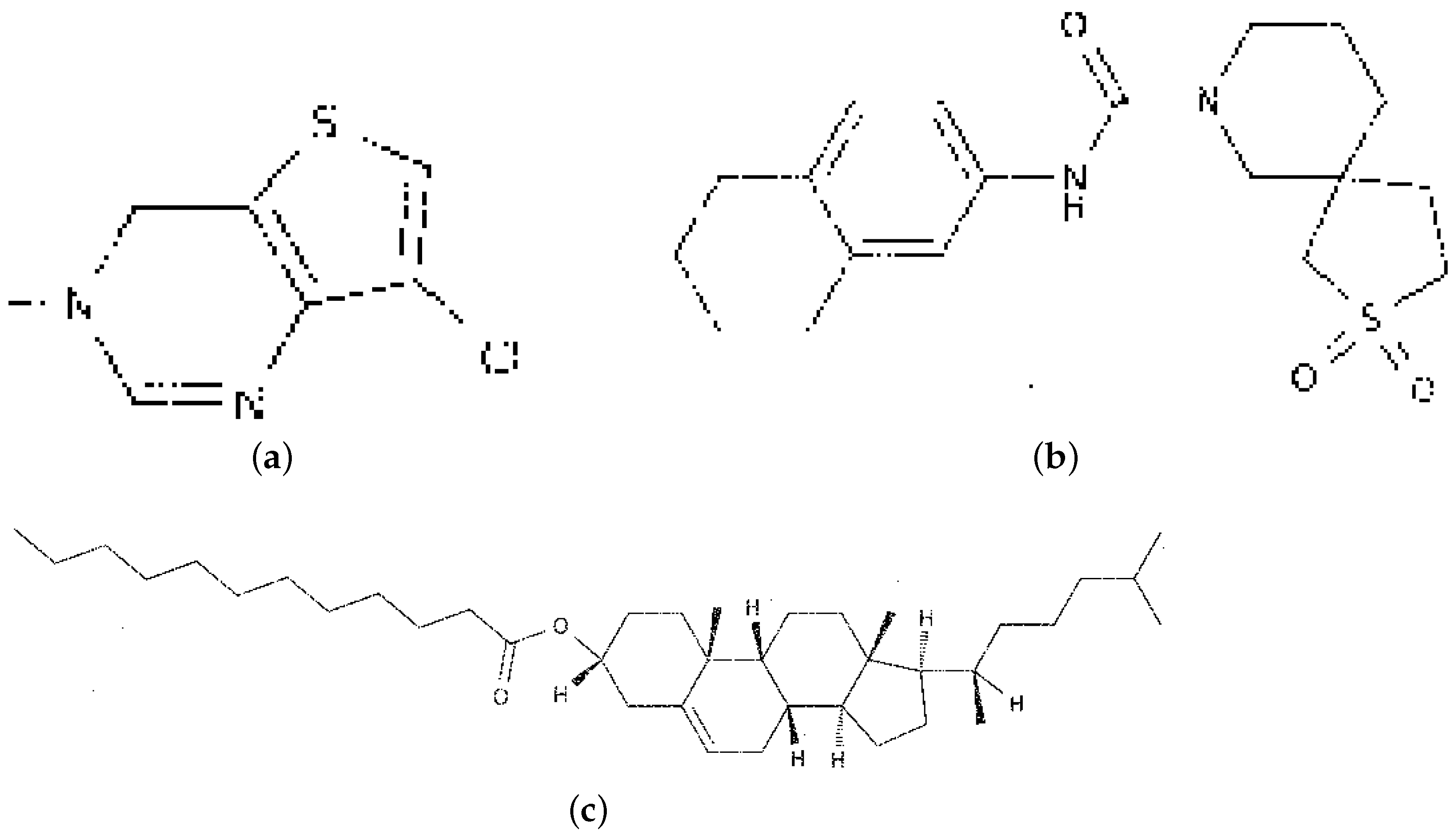
| Image Number & Real InChI | Model | Inference Results |
|---|---|---|
| Figure 10a | ICMDT | InChI = 1S/C7H7ClN2S/c8-7-9-4-6-5(10-7)2-1-3-11-6/h4H,1-3H2 |
| InChI = 1S/C7H7C1N2S /c8-7-9-4-6-5(10-7) | ResNet101d + Transformer | InChI = 1S/C7H7ClN2S/c8-7-9-4-6-5(10-7)2-1-3-11-6/h4H,1-3H2 |
| 2-1-3-11-6/h4H,1-3H2 | EfficientNetb0 + Transformer | InChI = 1S/C7H7ClN2S/c8-7-9-4-6-5(10-7)2-1-3-11-6/h4H,1-3H2 |
| ResNet50d + RNN | InChI = 1S/C7H7ClN2S/c8-7-9-4-6-5(10-7)2-1-9-11-8/h4H,1-3H2 | |
| EfficientNetb0 + RNN | InChI = 1S/C7H7ClN2S/c8-7-9-4-6-5(10-7)2-1-3-11-6/h5H,1-4H2 | |
| TNTD | InChI = 1S/C7H7ClN2S/c8-7-9-4-6-5(10-7)2-1-3-11-6/h4H,1-3H2 | |
| Figure 10b InChI = 1S/C19H26N2O3/ | ICMDT | InChI = 1S/C19H26N2O3/c1-13-3-6-15(7-4-13)21(2)19(23)12-24-16-8-9-17-14(11-16) 5-10-18(22)20-17/h8-9,11,13,15H,3-7,10,12H2,1-2H3,(H,20,22) |
| C1-13-3-6-15(7-4-13) 21(2)19(23)12-24-16- 8-9-17-14(11-16)5-10 | ResNet101d + Transformer | InChI = 1S/C19H26N2O3/c1-13-3-15(7-4-13)21(2)19(23)12-24-16-8-9-17-14(11-16) 5-10-18(22)20-17/h8-9,11,13,15H,3-7,10,12H2,1-2H3,(H,20,22) |
| -18(22)20-17/h8-9,11, 13,15H,3-7,10,12H2,1 -2H3,(H,20,22) | EfficientNetb0 + Transformer | InChI = 1S/C19H26N2O3/c1-13-3-6-15(7-4-13)21(2)19(23)12-24-16-9-17-14(11-16) 5-10-18(22)20-17/h8-9,11,13,15H,3-7,10,12H2,1-2H3,(H,20,22) |
| ResNet50d + RNN | InChI = 1S/C19H26N2O3/c1-13-3-6-15(7-4-13)21(2)19(23)-24-16-8-9-17(11-16) 5-10-18(22)20-17/h8-9,11,13,16H,3-7,10,13H2,1-2H3,(H,20,22) | |
| EfficientNetb0 + RNN | InChI = 1S/C19H26N2O3/c1-13-3-6-15(7-4-13)21(2)19(23)12-24-9-17-14(11-16) 5-10-18(22)20-17/h8-9,11,13,15H,3-7,12H2,1-2H3,(H,20,22) | |
| TNTD | InChI = 1S/C19H26N2O3/c1-13-3-6-15(7-4-13)21(2)19(23)12-24-16-8-9-17-14(11-16) 5-10-18(22)20-17/h8-9,11,13,14H,3-7,10,12H,1-2H3,(H,20,22) | |
| Figure 10c InChI = 1S/C39H68O2/ c1-7-8-9-10-11-12- 13-14-15-19-37(40) | ICMDT | InChI = 1S/C39H68O2/c1-7-8-9-10-11-12-13-14-15-19 -37(40)41-32-24-26-38(5)31(28-32)20-21-33-35-23 -22-34(30(4)18-16-17-29(2)3)39(35,6)27-25-36(33) 38/h20,29-30,32-36H,7-19,21-28H2,1-6H3/t30-,32-, 33-,34-,35-,36-,38+,39+/m1/s1 |
| 41-32-24-26-38(5) 31(28-32)20-21-33- 35-23-22-34(30(4) 18-16-17-29(2)3)39 (35,6)27-25-36(33) | ResNet101d + Transformer | InChI = 1S/C39H68O2/c1-7-8-9-10-11-12-13-14-15-19 -37(40)41-35-24-26-38(5)35(28-32)20-25-33-35-23 -22-34(30(4)18-16-17-39(35,6)27-25-36(33)38/h20, 29-30,32-39H,7-19,21-23H2,1-6H3/t30-,32-,33+,36-,38+,39-/m1/s1 |
| 38/h20,29-30,32- 36H,7-19,21-28H2, 1-6H3/t30-,32-,33+, 34-,35+,36-,38+, 39-/m1/s1 | EfficientNetb0 + Transformer | InChI = 1S/C39H68O2/c1-7-8-9-10-11-12-13-14-15-19 -46-32-24-26-33(5)31(28-32)23-21-33-35-23-22-34 (30(4)18–29(2)3)39(35,6)26-25-36(33)38/h20,29- 30,32-36H,7-19,21-28H2,1-6H3/t30-,35+,36+,38-,39-/m1/s1 |
| ResNet50d + RNN | InChI = 1S/C39H68O2/c1-7-8-9-10-11-12-12-12-15-19 -32-24-26-38(5)31(28-32)20-21-33-35-23-22-34(30 (4)18-16-17-29(2)3)39(35,6)27-25-36(33)38/h20, 29-30,32-36H,7-19,21-28H2,1-6H3/t30-,32-,33+,34+,35+,36-,38-,39-/m1 | |
| EfficientNetb0 + RNN | InChI = 1S/C39H68O2/c1-7-8-9-10-11-12-13-14-15-19 -37(40)41-32-38(5)31(23-32)20-23-22-21-33-35-34 (30(4)18-16-17-29(2)3)39(35,6)27-25-36(33)38/h20 ,29-30,7-19,21-28H2,1-9H3/t30-,32-,33-,34-,38-,39-/m1/s1 | |
| TNTD | InChI = 1S/C39H68O2/c1-7-8-9-10-11-12-13-16-15-19 -37(40)41-29-24-26-38(5)31(28-32)20-21-23-22-34 (30(4)18-18-17-29(2)3)39(35,6)27-25-36(33)38/h20, 29-30,32-36H,7-19,21-28H2,1-6H3/t30-,32-,33+,34+,35+,36-/m1/s1 |
Publisher’s Note: MDPI stays neutral with regard to jurisdictional claims in published maps and institutional affiliations. |
© 2022 by the authors. Licensee MDPI, Basel, Switzerland. This article is an open access article distributed under the terms and conditions of the Creative Commons Attribution (CC BY) license (https://creativecommons.org/licenses/by/4.0/).
Share and Cite
Li, Y.; Chen, G.; Li, X. Automated Recognition of Chemical Molecule Images Based on an Improved TNT Model. Appl. Sci. 2022, 12, 680. https://doi.org/10.3390/app12020680
Li Y, Chen G, Li X. Automated Recognition of Chemical Molecule Images Based on an Improved TNT Model. Applied Sciences. 2022; 12(2):680. https://doi.org/10.3390/app12020680
Chicago/Turabian StyleLi, Yanchi, Guanyu Chen, and Xiang Li. 2022. "Automated Recognition of Chemical Molecule Images Based on an Improved TNT Model" Applied Sciences 12, no. 2: 680. https://doi.org/10.3390/app12020680