Grid-Based Hybrid Genetic Approach to Relaxed Flexible Flow Shop with Sequence-Dependent Setup Times

Abstract

In this paper, a hybrid genetic algorithm implemented in a grid environment to solve hard instances of the flexible flow shop scheduling problem with sequence-dependent setup times is introduced. The genetic algorithm takes advantage of the distributed computing power on the grid to apply a hybrid local search to each individual in the population and reach a near optimal solution in a reduced number of generations. Ant colony systems and simulated annealing are used to apply a combination of iterative and cooperative local searches, respectively. This algorithm is implemented using a master–slave scheme, where the master process distributes the population on the slave process and coordinates the communication on the computational grid elements. The experimental results point out that the proposed scheme obtains the upper bound in a broad set of test instances. Also, an efficiency analysis of the proposed algorithm indicates its competitive use of the computational resources of the grid.

1. Introduction

A scheduling problem (SP) involves the efficient assignment of disposable resources (processors or machines) to complete one or several related tasks (jobs) over time [1]. SP is a relevant topic in science and engineering with a wide range of applications in diverse areas such as telecommunications [2], industry [3,4], health [5,6], agriculture [7], and education [8]. Due to its importance and impact on all aspects of human activity, SP is a well-studied problem in the scientific community. Many techniques and procedures have been proposed to solve its diverse variants. Almost any SP variant is NP-hard [9,10]. Its study is essential to provide better solutions, take advantage of technological development, and implement more efficient solution procedures.

A job shop SP (JSSP) is where a set of jobs, each composed of several operations, is processed on several machines without violating the precedence relations between the operations of all the jobs [11]. Two well-known JSSP variants are the flow shop SP (FSP) and the open shop SP (OSP). In a JSSP, jobs are processed on machines in identical order, visiting all or some of them. OSP has no precedence relations. Furthermore, an FSP is named as flexible FSP when a job uses only one machine available of those arranged in parallel in each stage of its processing sequence. These variants can be subject to several constraints derived from real problem conditions, such as (1) blocking constraints, if there is no intermediate storage (buffer) between consecutive machines, and the current machine processing the job is blocked until the next one is available [12]; (2) no-wait constraints, if all the operations of one job need to be processed without any interruption [13]; and (3) sequence-dependent setup time constraints, when the machines need to be adjusted (setup time) before processing their following jobs [14]. In particular, an SP with sequence-dependent setup times is among the most challenging classes of scheduling problems [15].

With the implementation of flexible manufacturing systems (FMS) [16] and the increased use of information technologies in Industry 4.0, flexibility on production lines has become crucial for achieving a companies’ objectives. Flexibility in FSP allows for the increasing of a factory’s capacities and also a reduction in the bottleneck impact on conflicting stages [17]. Therefore, the flexible FSP (FFSP) has been used to model real-world cases, like that described by Ramezanian et al. [18] for one tile factory with four stages (pressing, glazing, furnace, and sorting and packing) using four identical machines in each one. Also, Peng et al. [19] model an FFSP for the steelmaking process of an iron and steel complex in China which has three consecutive stages (steelmaking, refining, and continuous casting). Here, seven jobs were processed using several identical machines in each stage.

As with other scheduling problem variants, branch-and-bound-based techniques, heuristics, and metaheuristics have been used to solve FFSP instances. Only sequential and parallel algorithms have been implemented in all of them, and the use of distributed algorithms in grid environments has been scarcely documented in the existing literature. Furthermore, few manuscripts address the FFSP with sequence-dependent setup times, and they are restricted to particular cases as no-wait or permutation schedules. For example, Sankaran [20] describes a particle swarm optimization (PSO) algorithm used to solve several FFSP instances. This approach uses a random key scheme to transform the real-valued agents used by the PSO into valid schedules. The authors evaluate this proposal with several instances using several combinations of 30 and 100 jobs, two, four, and eight stages, and two, four, and ten parallel machines. Furthermore, Amiri [21] uses the same FFSP instances to evaluate several PSO-based versions such as standard PSO, passive congregation PSO, attraction repulsion PSO, discrete PSO, and hybrid discrete PSO with a local search (DPSO-LS).

In this paper, a relaxed FFSP with sequence-dependent setup time constraints is described as one 0–1 integer programming problem and then solved using an ensemble of three metaheuristics, including genetic algorithms (GAs), ant colony systems (ACO), and simulated annealing (SA). This ensemble runs in a grid-based environment using two clusters, where the candidate solutions are distributed in the grid cores.

The main contributions of this proposal are the following: (1) the implementation of a cooperative hybrid GA combining GA global search skills with both iterative and cooperative local search properties provided by SA and ACO to solve RFFSP instances; (2) that the binary representation of candidate solutions efficiently exploits the characteristics of the search approaches, unlike the known proposals where there is a mapping between the continuous and the discrete space, which is not guaranteed to maintain the properties of the search heuristic; (3) the use of an island model with a star-type connection to run the ensemble of heuristics in a grid-based environment. Furthermore, with a master-slave scheme, the evolutionary process is conducted in a master process. The local search is carried out in a set of slave processes distributed in a grid environment. Also, the master process distributes the population on the slave processes and coordinates the communication on the computational grid elements. The communication occurs in both directions using point-to-point communication. Finally, since, to the best of our knowledge, there are no instances in the existing literature for the optimization model under study, four instances (small, medium, and large) are designed to test the proposed ensemble.

The rest of this document is organized as follows: Section 2 describes the relaxed flexible flow shop problem with sequence-dependent setup times and presents a novel mathematical model to solve this problem. Section 3 introduces the grid-based algorithm used in this paper, the hybrid genetic algorithm in the grid environment, and the experimental results are discussed in Section 4. Finally, Section 5 contains the conclusions and future work of this proposal.

2. The Relaxed Flexible Flow Shop Problem Model with Sequence-Dependent Setup Times (RFFSP) Methods

The relaxed flexible flow shop problem (RFFSP) with sequence-dependent setup times consists of a set N = {1, 2, …, n} of n jobs that are processed by a set M = {1, 2, …, m} of m stages in serial. Each k-th stage, k ∈ M, has a set M_k = {m₁, m₂, …, m_k} of m_k identical parallel machines, where each j-th job, j ∈ N, in k-th stage, k ∈ M, can be processed in any i-th machine, i ∈ m_k. Each job requires m operations to be completed. One operation o_ijk of the j-th job is processed in the k-th stage using the i-th machine, taken from the set M_k of parallel machines, where each machine can only process one job at a time. Also, an operation being processed cannot be interrupted until it is finished. Each of the n jobs is first processed in stage 1, then in stage 2, and so on, indicating that a precedence order to process the job’s operations in each stage exists. The processing time of the j-th job in the k-th stage is defined as p_jk. Furthermore, each machine needs one setup time, that is, a time to be ready after processing one operation and starting the next. If the l-th and the j-th jobs are sequentially processed in the k-th stage by the i-th machine, this machine’s setup time is defined as ST_iljk. If the machines in one stage are identical, the setup time is defined as ST_ljk. In particular, if j is the first job assigned to the i-th machine in the k-th stage, its initial setup time is ST_0jk, and if l is its last job assigned, its setup time is ST_l0k.

One example of an RFFSP is described in [22] for a labeling company. The jobs are processed in seven stages (printing, labeling, lamination, die-cut, inject, and scan EPC). Each stage has several identical machines to execute its operations, and the job must be processed in sequence, starting with the printing stage. When a machine finishes processing a job, it needs to be cleaned, adjusted, and revised to verify if it has enough supplies to perform the next job.

2.1. Mathematical Model

The mathematical model introduced by [23] is used and adapted to the problem presented in this work. This adapted model uses inter-stage infinite buffers, which serve as temporary storage to place completed operations from an earlier stage, as machines cannot be blocked if other machines in later stages have not finished processing a job. The machine blocking constraint presented in [23] does not apply in this model.

The objective of the mathematical model, represented by the Equation (1), minimizes the maximum completion time (makespan, c_max) found in the sequence of jobs generated by the system in study. The makespan c_jm of the j-th job in the last stage m, is when it finishes its processing in the system ($c_{jm=s_{jm}+S{T}_{ljm}+p_{jm}}$) and its value is the sum of its start time s_jm, its processing time p_jm, and its setup time ST_ljm. Constraints in (2) indicate that for each j there is only one job l that immediately precedes j $\left(l\prec j\right)$ which is only assigned to a single machine i in stage k. Constraints in (3) point out all jobs are processed in a well-defined sequence by each machine in each stage. These complement the restrictions in (2), guaranteeing that jobs are executed in a well-defined sequence on each machine at each stage. It is only allowed to process the j-th job once in one machine for each stage.

$$Min{c}_{max}\left(s_{jm},p_{jm},S{T}_{ljm}\right)=Min\left[max\left(c_{jm}\right)\right]$$

(1)

s.t.

$${\displaystyle \sum }_{i=1}^{m_k}{\displaystyle \sum }_{l=0,l\ne j}^n{x}_{iljk}=1 \forall k,j$$

(2)

$${\displaystyle \sum }_{l=0,l \ne j}^n{x}_{iljk}={\displaystyle \sum }_{q=0,q \ne j}^n{x}_{ijqk} \forall k,i,j$$

(3)

$$c_{jk}\ge s_{jk}+p_{jk}+{\displaystyle \sum }_{i=1}^{m_k}{x}_{iljk}S{T}_{ljk} \forall j,l,k$$

(4)

$$c_{jk}-c_{j\left(k-1\right)}\ge p_{jk}+{\displaystyle \sum }_{i=1}^{m_k}{\displaystyle \sum }_{l=0}^n{x}_{iljk}S{T}_{ljk} \forall k>1,j$$

(5)

$$c_{max}\ge c_{jm} \forall j$$

(6)

$$x_{iljk}\in \left\{0,1\right\} \forall i,j,l,k$$

(7)

Constraints in (4) indicate that if a slack time between l-th and j-th jobs processed on the i-th machine of the k-th stage occurs, the makespan c_jk of the j-th job of the k-th stage can be increased [24]. The start time s_jk of the j-th job is taken when it begins your setup time. Constraints in (5) define the precedence restrictions of each j-th job’s operations and guarantee that each job is processed in all stages. Constraints in (6) indicate that each job has a makespan less than or equal to the maximum makespan. Finally, relations in (7) restrict the x_iljk to be binary variables only: x_iljk = 1, if job j is assigned to machine i in stage k where job l is its predecessor job, otherwise x_iljk = 0.

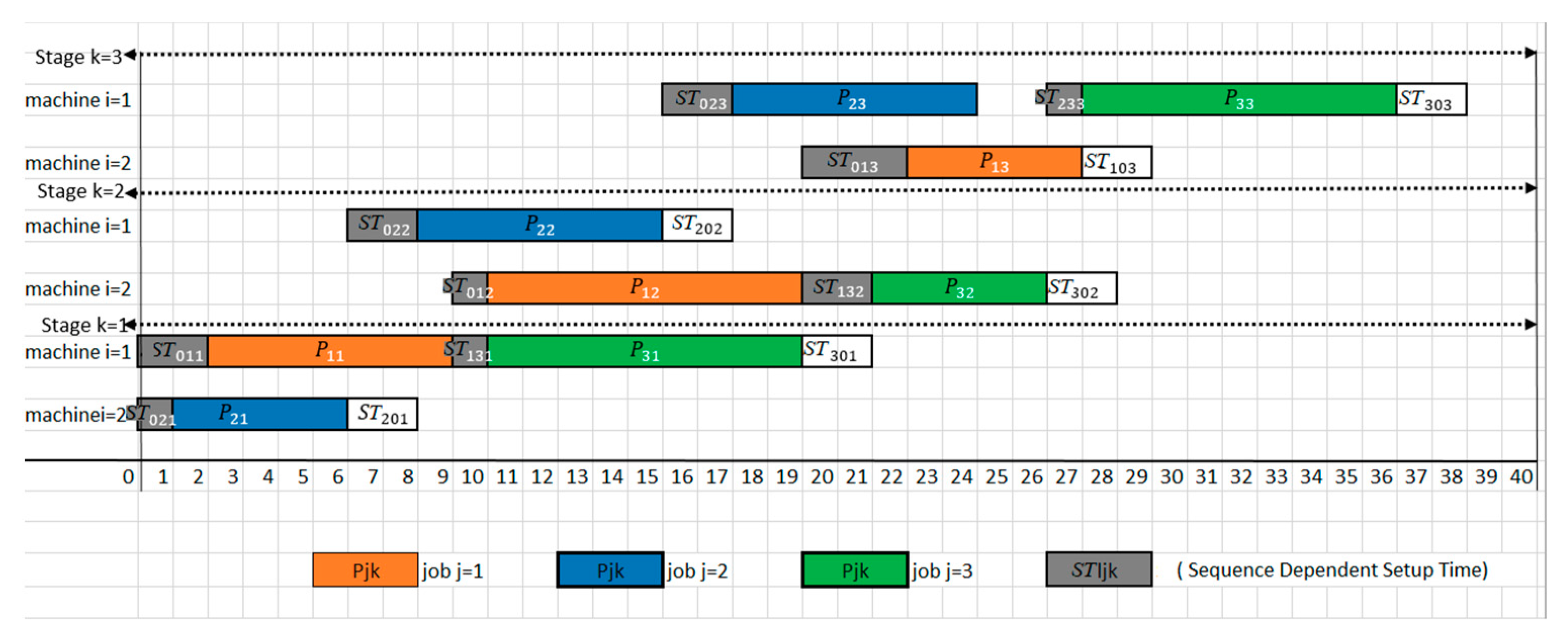
2.2. Disjunctive Graph Model

Figure 1 shows a disjunctive graph G modeling the RFFSP for an example of two jobs (N = 2) processed in three stages (M = 3), each stage with two identical machines (M_k = 2). G is composed of three sets representing the conjunctive arcs A, the disjunctive arcs E, and the graph nodes O_i,j,k. These nodes identify the jobs’ operations. Set A includes three arcs subsets, each by one job. For example, the subset of arcs joining O_{1|2}11, O_{1|2}12, and O_{1|2}13 operations correspond to job 1. Also, the conjunctive arcs define the precedence relation between operation pairs. For example, O_{1|2}11 must be processed before O_{1|2}12, and O_{1|2}12 before O_{1|2}13. Each node in G is depicted using a blue circle with a dashed line, and inside it, two gray circles with continuous lines represent the parallel machines used in this stage. The processing time p_jk of each operation is also depicted in the blue circle, p₁₁ = 7 for O_{1|2}11 in Figure 1, for example. Furthermore, G uses two fictitious operations, labeled as input and output, to specify the start and end of each job’s processing time.

The operations processed in the same stage define a clique, since they are joined using disjunctive arcs. For example, O_{1|2}11, O_{1|2}21, and O_{1|2}31 are processed in stage one. It is necessary to find the operations processing sequence at each stage, selecting one of the parallel machines for each operation. Once this sequence is found, the disjunctive arches will become conjunctive arcs.

Table 1. Setup times for the RFFSP shown in Figure 1.

STljk	j = 1	j = 2	j = 3	0 (Cleaning)
Stage 1 (STljk)
0 (start)	ST011 = 2	ST021 = 1	ST031 = 3	ST001 = 0
l = 1	ST111 = 0	ST121 = 2	ST131 = 1	ST101 = 0
l = 2	ST211 = 1	ST221 = 0	ST231 = 1	ST201 = 0
l = 3	ST311 = 2	ST321 = 3	ST331 = 0	ST301 = 0
Stage 2 (STljk)
0 (start)	ST012 = 1	ST022 = 2	ST032 = 3	ST002 = 0
l = 1	ST112 = 0	ST122 = 3	ST132 = 2	ST102 = 0
l = 2	ST212 = 1	ST222 = 0	ST232 = 1	ST202 = 0
l = 3	ST312 = 3	ST322 = 3	ST332 = 0	ST302 = 0
Stage 3 (STljk)
0 (start)	ST013 = 3	ST023 = 3	ST033 = 1	ST003 = 0
l = 1	ST113 = 0	ST123 = 2	ST133 = 1	ST103 = 0
l = 2	ST213 = 2	ST223 = 0	ST233 = 1	ST203 = 0
l = 3	ST313 = 3	ST323 = 2	ST333 = 0	ST303 = 0

shows the setup times for each operation of the example shown in Figure 1.

Figure 2 shows a solution to the example previously described. It can be seen that the sequence of the operations in each stage is defined, disjunctive arcs are now conjunctive, and only one machine has been assigned to each operation. Furthermore, the processing and setup times are depicted in each arc with black and red numbers, respectively.

A Gantt diagram of the scheduling of the solution described previously is shown in Figure 3, where the job’s operations are outlined using the same color. In this diagram, the solution fulfills the precedence constraints between pairs of operations of the same job, and each operation starts its processing until the machine setup time is accomplished. The solution of any RFFSP instance can be reached using the mathematical model described in the previous section.

The following section describes the grid-based hybrid genetic approach to solve the relaxed flexible flow shop with sequence-dependent setup times expressed using the mathematical model previously detailed.

3. Hybrid Genetic Algorithm in Grid Environment (HGAG) to the Relaxed Flexible Flow Shop with Sequence-Dependent Setup Times

The cooperative hybrid genetic algorithm in a grid environment, called HGAG, combines the global search skills of a genetic algorithm (GA) with an iterative local-search, provided by a simulated annealing algorithm (SA), and the cooperative local-search implemented by an ant colony system (ACS) to solve RFFSP instances. HGAG is implemented using the Grid Morelos infrastructure (Figure 4). This scheme increases the solution refinement by combining the two local-search procedures.

3.1. Hybrid Genetic Algorithm in Grid Environment (HGAG)

The HGAG designed and developed in this work used to solve the RFFSP is presented in Algorithm 1, the steps of which are detailed in the following paragraphs. Also, the main elements of the GA are described. Multiple instances of the HGAG run in the computational grid. The algorithm automatically assigns identifiers unequivocally for each running process. These identifiers are used to select the HGAG code segment to be run: if it is zero, the code segment chosen is for the master process. Otherwise, the code segment selected is for the slave processes.

Algorithm 1 Hybrid Genetic Algorithm in Grid Environment (HGAG)
1.	Note: blocking routines are used for sending and receiving messages
2.	Function HGAG $\leftarrow$ (Processid, idmax)
3.	if (Processid == ProcSlave) then
4.		$S_{ant}\leftarrow \{\varnothing \}$
5.		$C_{max}\left(S_{BestLocal}\right)\leftarrow 999999$
6.	end if
7.	Repeat
8.		if (Processid == ProcMaster) then
9.			ReceiveF(Processi, population[individuali], blocking), $i=1,2,\cdots ,i{d}_{max}$
10.			population $\leftarrow$selectionF(rouleteOp, population)
11.			population$\leftarrow$crossoverF(crossoverR, circularOp, population)
12.			SendF(Processi, population [individuali]), $i=1,2,\cdots ,i{d}_{max}$
13.		Else
14.			$S_{ant}^{\prime }\leftarrow ACS\left(h,\alpha ,\beta ,\gamma ,\delta ,p,q,UB,S_{ant}\right)$
15.			$S_{metal}\leftarrow \left(S_{ant}^{\prime }{f}_{\to }SA\right)$
16.			$S_{metal}^{\prime }\leftarrow SA\left(t_o,m,\mu ,t_f,S_{metal}\right)$
17.			$S_{individual}\leftarrow \left(S_{metal}^{\prime }{f}_{\to }individual\right)$
18.			$S_{BestLocal}=min\left(C_{max}\left(S_{BestLocal},S_{ant},S_{ant}^{\prime },S_{metal}^{\prime }\right)\right)\to individual$
19.			$SendF\left(ProcMaster,S_{individual}\right)$
20.			$ReceiveF\left(ProcMaster,S_{individual}^{\prime },blocking\right)$
21.			$S_{ant}\leftarrow \left(S_{individual}^{\prime }{f}_{\to }ACS\right)$
22.		end if
23.	until (number of generations)
24.	if (Processid == ProcMaster) then
25.		ReceiveF (Processi, population [individual i], $i=1,2,\cdots ,i{d}_{max}$
26.		SBestGlobal $\leftarrow$ min(Cmax(population[individuali])),$i=1,2,\cdots ,i{d}_{max}$
27.		return (SBestGlobal)
28.	Else
29.		SendF (ProcMaster, SBestLocal)
30.	end if
31.	end Function HGAG

• Initialization stage

Line 2: The algorithm receives the process identifier (Process_id) and the number of the available process (id_max) as input parameters.

Lines 3–6: If the Process_id corresponds to one slave process, the Ant Colony System and the corresponding makespan are initialized (S_ant = Ø, C_max(S_BestLocal) = 999999).

• Evolutionary stage

Lines 7–23: This is the main procedure with regard to the HGAG finding the best solutions for the RFFSP. If Process_id corresponds to a master process, lines 9–12 are carried out; otherwise, lines 14–21 are run. This procedure is run until a stop condition is reached.

• Master process

Line 9: The master process waits until the slave processes have sent their candidate solutions. With these solutions, it builds the initial population as a vector of individuals. The population size is defined by the variable id_max = P_max − 1, where P_max is the number of processing cores. The population is initialized with the messages sent by the slave processes (Process₁ to Process_idmax). Each message sent is one individual encoding the best solution found by SA (Algorithm 4) and ACS (Algorithm 2). In particular, the receiveF function has a blocking behavior; that is, while the master process waits to receive messages, it is kept blocked until all of them are received.

Line 10: A new population is generated by applying the selection operator using the roulette method. The aim is to have the best-adapted individuals in the new population.

Line 11: A new population is generated as a result of applying the circular crossover operator. A crossover rate is defined to explore the solutions space of the new population.

Line 12: The new population is distributed to the slave processes: individual₁ is sent to Process₁, individual₂ is sent to Process₂, and so on until the entire population is sent. All the slave processes wait for an evolved solution and then apply the mutation operator.

• Slave process

Line 14: The ACS (Algorithm 2) is used to compute an improved solution based on that received from the master process. ACS uses a cooperative mutation guided by the pheromone traces based on the initial solution and returns S′_ant as the best-found solution.

Line 15: The S_metal solution is calculated using a transformation function to convert the best solution found by ACS (S′_ant) to be used as the SA initial solution. S_metal is equivalent to S′_ant since the transformation function does not alter the scheduling. It only realizes a context change on the solution representation.

Line 16: S′_metal is calculated using SA (Algorithm 4). The SA parameters are the follows:

• t₀ is the initial temperature.
• m is the Markov chain length.
• µ is the frozen coefficient.
• t_f is the final temperature
• S_metal is the SA initial solution.

This routine applies an iterative mutation guided by the initial solution S_metal. SA returns S′_metal as its best-found solution.

Line 17: S_individual is computed using a transformation function to convert the best solution found by SA (S′_metal) in one GA individual. This transformation enables SA to send S′_metal to the master process to build a new population.

Line 18: The best solution between those found by ACS and SA is stored in the variable S_BestLocal.

Line 19: The best local solution is sent to the master process. At this point, the master process waits to receive all solutions from the slave processes.

Line 20: Every slave process waits for the master process to send it S′_individual. The ReceiveF function blocks the slave process until a solution is received.

Line 21: S_ant is computed using a transformation function. This transformation prepares the algorithm for the next generation that begins with a cooperative mutation with ACS.

• Final stage

Line 27: Finally, the best global solution found by HGAG is returned (S_mBEstGlobat).

• Population Construction

The HGAG population is distributed in the grid with a 1:1 ratio, i.e., one individual for each process p generated in the computational grid. A single process is assigned to each core that the processor contains. The master process stores the solutions found by the other process in a solutions vector. The master process receives the best solutions found by each slave process and assigns these solutions to the vector to build a new population in each generation.

The symbolic representation of a solution encoded as a GA individual is presented in Figure 5. This representation consists of a data structure storing the sequence of operations in each machine and each stage, and the scheduling obtained using all start times s_jk for each operation. With the scheduling, the Makespan C_jk of each job is obtained for the last stage to compute the maximum Makespan C_max. In Figure 5, the individual encodes the solution depicted in Figure 2. The scheduling of this solution is shown in Figure 3. In this case, C_max = 36. For the sake of simplicity, the individual is represented in a sequence of operations for each machine, as follows:

$$O_{111}\to O_{131}\to O_{221}\to O_{122}\to O_{212}\to O_{232}\to O_{123}\to O_{133}\to O_{213}$$

• Selection Operator

A roulette-based selection operator [25] is used in the HGAG, where the fittest individuals are more likely to be selected. As the fitness function (Equation 1) minimizes the makespan, the fittest individuals have the lowest cost. The cost inverse is computed making the fittest individuals correspond to those more likely to be selected. This procedure is used in line 10 of Algorithm 1. The steps used by this operator are as follows:

• The probability prob_i to select the individual_i is proportional to its relative adaptation, which is calculated as follows:

  $$pro{b}_i=\frac{C_{max}{\left(individua{l}_i\right)}^{-1}}{{{\displaystyle \sum }}_{j=1}^{i{d}_{max}}{C}_{max}{\left(individua{l}_j\right)}^{-1}}$$

  (8)

  where $C_{max}{\left(individua{l}_i\right)}^{-1}$ is the cost inverse for individual_i, and ${\displaystyle \sum }_{j=1}^{i{d}_{max}}{C}_{max}{\left(individua{l}_j\right)}^{-1}$ is the total fitness of the population.
• Cumulative probabilities are calculated for each individual_i, as follows:

  $$acu{m}_i=pro{b}_1+\dots +pro{b}_i$$

  (9)
• The selection criterion consists of generating a random number r uniformly distributed over an interval [0, 1].
• The individual selected is located in the population as follows:

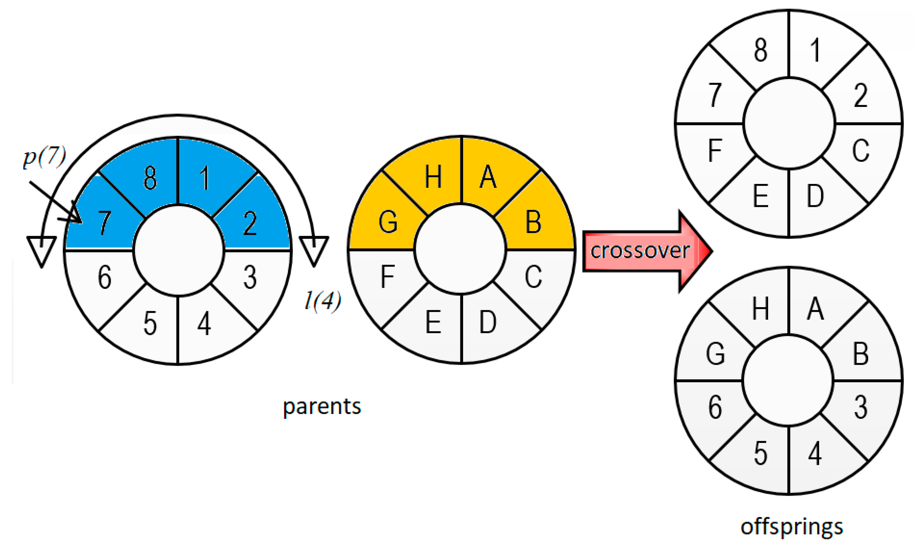
  $$se{l}_i=acu{m}_{i-1}<r<acu{m}_i$$

  (10)

Steps one and two are applied once, and the remaining are used each time an individual needs to be selected based on their fitness value.

• Crossover operator

The crossover operator exchanges the chromosomes of two parents to create two new offspring [26]. This crossover operator uses a roulette procedure and a crossover rate ∈ (0, 1], and, by taking two parents (parent_i, parent_i+1) with i = 1, 2, …, idmax, produces two offspring (child_i, child_i+1).

An example is shown in Figure 6, where parent₁ = {1, 2, 3, 4, 5, 6, 7, 8} and parent₂ = {A, B, C, D, E, F, G, H} with length 8, and the crossing point and crossing length of the parent₁ are p(7) and l(4), respectively, resulting in two children, child₁ = {1, 2, C, D, E, F, 7, 8} and child₂ = {A, B, 3, 4, 5, 6, G, H}. This procedure is applied in line 11 of Algorithm 1.

For example, if the solution shown in Figure 5 is used as one parent:

Parent 1: $O_{111}\to O_{131}\to O_{221}\to O_{122}\to O_{212}\to O_{232}\to O_{123}\to O_{133}\to O_{213}$ and, in conjunction with other parent solution:

Parent 2: $O_{121}\to O_{211}\to O_{231}\to O_{122}\to O_{132}\to O_{212}\to O_{113}\to O_{133}\to O_{223}$ are used with the crossover operator, the next offspring are created:

Offspring 1: $O_{111}\to O_{131}\to O_{221}\to O_{122}\to O_{132}\to O_{212}\to O_{123}\to O_{133}\to O_{213}$

Offspring 2:$O_{121}\to O_{211}\to O_{231}\to O_{122}\to O_{212}\to O_{232}\to O_{113}\to O_{133}\to O_{223}$ The main characteristic of this crossover operator is that it preserves the sequence order from stages 1 to n so that a circular crossover at a single point only exchanges the order of the jobs between stages, not the order of the stages, to avoid infeasible solutions.

HGAG works with distributed processing. The distribution, communication, synchronization, and cooperation of the processes generated to execute the algorithm are explained below.

HGAG uses MPI to execute processes on the Grid integrated by the Cuexcomate and the Texcal clusters (Figure 4). Each process is assigned to a single core through a uniform distribution when executing 5, 10, 15, 30, and 60 processes in a single cluster. If 120 processes are running, two clusters are used. Furthermore, it is possible to allocate more than one process per core, known as overhead [27], when 240 processes are executed, which can double the grid capacity. The architecture used is master/slave, where the master process collects and distributes the GA population, and the slave processes send and receive new solutions.

As shown in Figure 4, the selection and crossover operators are conducted by the master process, and the mutation operations are running on the slave processes through the ACO and SA algorithms described in Section 3.2 and Section 3.3, respectively.

The distribution of both HGAG and the instances is performed using the Grid Morelos distributed file system. Before executing the algorithm, copies of code and instances are first sent to the master nodes of both clusters (Cuexcomate and Texcal). Then, the distributed file system sends the input data to all the slave nodes in the Grid.

Communication between the master and slave processes is implemented using MPI functions and the TCP/IP protocol. Additionally, communication between geographically distant clusters is implemented using a VPN network, which groups them under the same network segment, allowing transparent communication.

As shown in Figure 7, the processes generated by HGAG communicate between the master process and the slave processes at specific times. The algorithm begins by reading the benchmark file of the Distributed File System (DFS), then the slave processes generate the first solutions applying ACS and refining with SA. The solutions found are sent to the master process in a many-to-one relationship to build the initial population of the GA. Selection and crossover are applied below to explore the solutions space. Subsequently, the master process distributes individuals of a one-to-many relationship to the slave processes that in turn transform the solution to apply ACS and SA for the exploitation of the solutions space. This process is repeated until the number of generations is complete. Finally, the slave processes send the best found solution to the master process, which receives them and selects the best global solution of the HGAG algorithm.

The information exchange uses a message-passing mechanism where one sends and the other receives, working as follows:

• The mechanism has a blocking behavior, i.e., while a process waits to receive messages, it keeps waiting (blocked) until it gets them.
• The slave process sending a message is blocked while depositing it in the master process queue (buffer), continuing its processing once the message has been delivered.
• The master process blocks while reading the messages from its buffer.
• If the receiving process reads a message before it is ready, it blocks until the message is completed.
• When the master process receives messages, it must wait for each slave process in sequential order.
• When the slave processes receive a message, they must wait for the master process to distribute the results in sequential order and then wait their turn.

3.2. Ant Colony System Algorithm

Algorithm 2 generates the cooperative-local search by applying an ant colony system (ACS) [28]. The ACS is used by HGAG, as is shown in line 14 of Algorithm 1.

Algorithm 2 ACS (Ant Colony System)
1.	Function ACS (h, α, β, γ, δ, p, q, UB, Sant)
2.		τ0 $\leftarrow$ (n.m.k.UB)−1
3.		τr,s $\leftarrow$ τ0, ∀arc ∈ G(V, A)
4.		τr,s $\leftarrow$ [Cmax(Sant)]−1,∀arc ∈ Sant
5.		Cmax(SBestLocal) $\leftarrow$ 999999
6.		Repeat
7.			while∀ (antk), con k = 1, 2, …, h
8.					S[antk] =BuildSolution(α, β, γ, q, τr,s,antk)
9.			end while
10.			SBestLocal $\leftarrow$ min(Cmax(SBestLocal), Cmax(S[antk])), k = 1, 2, …, h
11.			for (antk), k = 1, …, h
12.				for (arc(r, s)) ∈ S[antk]
13.					if arcr,s ∈ SBestLocal then
14.						τr,s $\leftarrow$ (1 − δ). τr,s+ δ.Δτr,s
15.					Else
16.						τr,s $\leftarrow$τr,s
17.					end if
18.				end for
19.			end for
20.		until(p)
21.		return (SBestLocal)
22.	end Function LCS

The ACS elements are described as follows:

Line 1: ACS receives the following parameters:

• h is the number of ants.
• α is the importance coefficient alpha.
• β is the importance coefficient beta.
• γ is the evaporation coefficient for the local transition.
• δ is the evaporation coefficient for the global transition.
• q is the coefficient to divide the exploration and exploitation rates.
• p is the stop criterion of the algorithm.
• UB is the best-known quote in the literature.
• S_ant is the ACS initial solution.

Line 2: The minimum pheromone value τ₀ used in each arc of the solution depicted in Figure 2 is defined. τ₀ is computed using the problem values (n, m, k) and its best upper bound known.

Line 3: The τ₀ value is assigned to each graph arc in Figure 2.

Line 4: Extra pheromone is deposited on the arcs of the initial solution received (S_ant), which is computed using the inverse of its fitness value. If S_ant is an empty solution, no extra pheromone is deposited.

Line 5: The makespan of the initial S_BestLocal solution is set using a maximum value.

Lines 6–20: This is the local search procedure involving the generation of solutions for the k ants, the evaporation of pheromone step by step, the updating of the best solution, and the adding of pheromone to the best solution in a cycle of p iterations.

Lines 7–9: The S_ant solutions are generated for each ant using the BuildSolution function with α, β, γ, q, τ_r,s, and ant_k as parameters. These solutions are stored in a vector S[ant_k] with k = {1, …, h}. The BestSolution function is described in Algorithm 3.

Line 10: In each iteration, the best solution with the lowest cost is identified, and its path is assigned to the S_BestLocal variable.

Lines 11–19: All solutions in the vector S[ant_k] are updated by evaporating and depositing pheromone only in those arcs that belong to the best solution found, where δ ∈ (0, 1] is an evaporation coefficient.

Line 21: At the end of the local search procedure, the S_bestLocal solution is returned.

The BuildSolution function is described in Algorithm 3, which is used to create the solutions for each ant_k. Its elements are explained in the following paragraphs:

Algorithm 3 Local Cooperative Search–BuildSolution()
1.	Function BuildSolution(α, β, γ, q, τr,s, k)
2.		r $\leftarrow$ input
3.		Sk $\leftarrow${r}
4.		Repeat
5.			r $\leftarrow$ random [0, 1]
6.			ifs∈Sk(r) ∧r ≤ q ∧ s ∉ tabuk then
7.				Sigkr,s $\leftarrow$ max s ∉ Sk(r)[ (τr,s) α.(nr,s)β ]
8.			else ifs∈Sk(r) ∧r > q ∧ s ∉ tabuk then
9.				Sigkr,s $\leftarrow$ roulette(((τr,s)α.(nr,s)β)/(∑u ∈ Sk(r)((τr,u)α.(nr,u)β)
10.			Otherwise
11.				Sigkr,s $\leftarrow$ 0
12.			end if
13.			Sk = Sk + sigs
14.			τr,s = (1-γ). τr,s + γ.τ0
15.			s $\leftarrow$ r
16.		until (r == exitCondition)
17.		return (Sk)
18.	end Function BuildSolution

Line 1: The algorithm receives α, β, γ, q, k as parameters.

Line 2: The ant k is placed in the initial arch.

Line 3: The initialization of the solution of ant k (S_k) by adding the first arc r visited.

Lines 4–16: This is the core section of the algorithm. The ant k traverses the graph, node by node, until it reaches the final node.

• Line 5: A random number r uniformly distributed between 0 and 1 is generated.
• Lines 6–11: A tabu list [29] is first used to build the set arc_r,s with the arcs joining the neighborhood of non-visited and reachable nodes of the ant k placed in node r s ∈ N_k(r). Then, another uniformly distributed random number q ∈ [0, 1] is generated and used to determine if exploitation or exploration is conducted. If r ≤ q, the ants apply their knowledge in terms of the pheromone amount (τ_r,s) and the transition costs (η_r,s). The next best arc with the largest amount of pheromone and a lower transition cost is selected. On the other hand, if r > q, a probability of choosing the next arc arc_r,s is obtained using a roulette-based selection.
• Line 13: The selected node s is added to the solution S_k.
• Line 14: As ant k advances from node r to node s, the pheromone is dissipated to make it less attractive to the following ants, allowing it to select other arcs not yet explored.
• Line 15: Ant k advances to the selected node s.

Line 17: The algorithm returns the solution S_k of ant k.

3.3. Simulated Annealing Algorithm

Algorithm 4 implements the iterative local search by applying a simulated annealing (SA) algorithm [30]. SA is applied by HGAG, as shown in line 16 of Algorithm 1. In each SA iteration, the Metropolis cycle uses the Boltzmann probability function as an acceptance criterion, computed using the temperature control parameter T, avoiding local optimum since it cannot accept improved solutions. Its elements are described in the following paragraphs:

Algorithm 4 SA (Simulated Annealing)
1.	Function SA(to, m, µ, tf, Smetal)
2.		T$\leftarrow$ To
3.		Cmax(SBestLocal) $\leftarrow$ 999999
4.		Srecent $\leftarrow$ Smetal
5.		Repeat
6.			fori, i = 1, 2, …, mdo
7.					Snew $\leftarrow$N(Srecent)
8.					if (CmaxSnew) ≤ Cmax(Srecent)) then
9.						Srecent $\leftarrow$Snew
10.						if (Cmax(Srecent) ≤ Cmax(SBestLocal)) then
11.							SBestLocal $\leftarrow$ Srecent
12.						end if
13.						else if
14.							Sdif $\leftarrow$ Cmax(Snew) −Cmax(Srecent)
15.							r $\leftarrow$ random [0, 1]
16.							if (r ≤ $e^{\frac{-S_{dif}}{T}}$) then
17.								Srecent$\leftarrow$Snew
18.							end if
19.						end if
20.				end for
21.				T$\leftarrow$ T. µ
22.				until (T ≤ Tf)
23.				return (SBestLocal)
24.	end Function SA

Line 1: SA receives the following parameters:

• t₀ is the initial temperature.
• m is the Markov chain length.
• µ is the frozen coefficient.
• t_f is the final temperature
• S_metal is the SA initial solution. This is the solution found by the ACS algorithm.

Line 2: The temperature T is initialized to a temperature T_o that will be decreased as the search progresses.

Line 3: The makespan of the initial S_BestLocal solution is set using a maximum value.

Line 4: The S_recent solution is initialized to the S_metal value.

Lines 5–22: This is the external cycle of the SA algorithm. This cycle updates the temperature control parameter and ends when the current temperature T is lower than the final temperature T_f. Lines 6–20: This is the Metropolis internal cycle. The Markov chain length determines its number of iterations.

• Line 7: A new solution S_new is created using a local search in the neighborhood of S_recent N(S_recent).
• Lines 8–12: If the objective function cost, defined in Equation (1), of the solution S_new is not greater than those of the S_recent solution, S_new replaces S_recent. S_recent always takes the best solution found. Furthermore, the S_bestLocal solution is updated with S_new.
• Lines 13–19: On the other hand, if the objective function cost of the solution S_new is greater than those of the S_recent solution, the Boltzmann criterion is used to accept the S_new solution as the S_recent solution. This criterion allows escaping from local optimums and the continued exploration of the solution space.

Line 23: The algorithm returns the S_bestLocal solution.

• Solution Representation

The SA candidate solution representation is the same as those used in the HGAG. In Figure 5, the sequence of the operations depicted in Figure 5 is:

$$O_{111}\to O_{131}\to O_{221}\to O_{122}\to O_{212}\to O_{232}\to O_{123}\to O_{133}\to O_{213}$$

The neighborhood structure used to find new candidate solutions is based on exchanging pairs of adjacent operations processed on the same machine or different machines. An example of one exchange in the same machine is as follows:

$$O_{131}\to O_{111}\to O_{221}\to O_{122}\to O_{212}\to O_{232}\to O_{123}\to O_{133}\to O_{213}$$

On the other hand, an example of an exchange of pairs of operations processed in different machines is as follows:

$$O_{221}\to O_{131}\to O_{111}\to O_{122}\to O_{212}\to O_{232}\to O_{123}\to O_{133}\to O_{213}$$

It is necessary to indicate that another machine executes the operation. Once the correction is made, the new neighboring solution is available:

$$O_{121}\to O_{131}\to O_{211}\to O_{122}\to O_{212}\to O_{232}\to O_{123}\to O_{133}\to O_{213}$$

4. Experimental Results

In this section are the experimental results of the hybrid genetic algorithm in grid environment (HGAG).

4.1. Platform of Experimentation

Grid Morelos is one of the first Mexican grids [31]. This grid is a homogenous platform constituted by two high-performance computer clusters, geographically distant (14.37 km) between them, and placed in the Morelos State. The main elements of the grid are the Cuexcomate and Texcal clusters. The Cuexcomate cluster is located at the Autonomous University of Morelos State (UAEM) in Cuernavaca Morelos, Mexico. The Texcal cluster is located at the Polytechnic University of Morelos State (UPEMOR), in Jiutepec, Morelos, Mexico. An open virtual private network integrates the clusters in a grid environment. Each cluster has its nodes, but the cluster Cuexcomate and the cluster Texcal have similar characteristics. The communication between these clusters is via a wireless WAN link between institutions implemented via a point-to-point microwave link with ISM frequency bands with 30 Mbps bandwidth. The grid software includes an OS Centos Linux 5.5, 64 bits, a gcc 4.1.2 compiler, an OpenMPI 1.8, an MPICH2, an Intel compiler MPI 12.0, a Ganglia 3.1.7, NFS-utils 1.0.9, VLAN, and Torque + Maui. The cluster communication uses a Switch 3COM 24/10/100/1000, a Switch InfiniBand Mellanox, 18 ports, 40 Gb/s QDR, and each cluster node uses an InfiniBand card 40 Gb/s. Each cluster has a master node with two Intel Xeon, Six-Core 3.06 GHz (12 cores), 12 MB cache, 6 HD 7200 RPM, 12 TB, 24 GB RAM. Furthermore, each cluster has four slave nodes with a two Intel Xeon Six-core 3.06 GHz (12 cores), 12 MB cache, 1 HD 7200 RPM, 500 GB, 24 GB RAM, InfiniBand card 40 Gb/s. In summary, the Grid Morelos has ten nodes and 120 cores.

4.2. Generation of Test Instances

When searching the existing literature, no instances were found with which the algorithm proposed in this manuscript could be compared. This is because the optimization model used in the present work is an adaptation of that defined in [23]. To the best of our knowledge, there is no similar algorithmic approach to comparing results. The model most similar to the one presented in [23] only analyzes a small-size instance that uses restrictions for machine blocking, this set of restrictions does not apply in this work in the optimization model that is resolved. Therefore, medium-size and large-size instances of the optimization model were generated, which allowed us to evaluate the performance of the HGAG in a high-performance computing environment and above 120 parallel processes.

According to the number of jobs, the benchmarks used are classified in the literature as small, medium, and large instances [32,33]. This work randomly generates benchmarks to solve the RFFSP described in Section 2. Based on [33], these benchmarks are also randomly generated using a proprietary program codified in the C language. The benchmarks are generated with the following characteristics:

• Five groups of jobs N = {20, 40, 60, 80, 140};
• Three groups of stages K = {2, 4, 8};
• Four groups of machines M = {2, 3, 4, 5};
• Processing times p_jk uniformly distributed in the range (1–99);
• Setup times ST_ljk, uniformly distributed in the ranges (1–25), (1–50), (1–00), and (1–125). These values correspond to 25%, 50%, 100% and 125% of ratio, according to the processing times.

The nomenclature, defined in this work, to name the benchmarks is the following:

RFFS_SDST_nxmxk xr _b

where RFFSP_SDST means relaxed flexible flow shop problem with sequence dependent setup times, n is the number of jobs, m is the number of stages, k is the number of parallel machines on each stage, r is the ratio of setup time, dependent on the sequence related to the processing time, and b is the problem number which can be from 1 to 5.

Five benchmarks are generated to create sets of five instances, to be solved with the HGAG.

Table 2. Instances for tuning the HGAG.

INSTANCES SET	NAME	Description	SIZE
1.	RFFS_SDST_20 × 4 × 4 × 25	n = 20, m = 4, k = 4, STljk = 25%	Small
2.	RFFS_SDST_40 × 4 × 4 × 25	n = 40, m = 4, k = 4, STljk = 25%
3.	RFFS_SDST_60 × 4 × 4 × 25	n = 60, m = 4, k = 4, STljk = 25%	Medium
4.	RFFS_SDST_80 × 4 × 4 × 25	n = 80, m = 4, k = 4, STljk = 25%
5.	RFFS_SDST_140 × 4 × 4 × 25	n = 140, m = 4, k = 4, STljk = 25%	Large

shows these instances. Readers can access the data of the instances that are resolved in this work in [34].

4.3. HGAG Sensibility Analysis

The HGAG has different parameters that must be tuned to find the appropriate values to get the best algorithm performance. The sensibility analysis is carried out with an automatically distributed tuning methodology. Three metaheuristics are used in the HGAG: one cooperative genetic algorithm, an ant colony system algorithm (ACS), and a simulated annealing algorithm (SA). For each algorithm, its input parameters are tuned. First, the GA parameters to be tuned are (1) the population size P, which is directly proportional to the number of grid processors, (2) the selection operator S, (3) the crossover-rate C, and (4) the number of generations G. Next, the ACS parameters to be tuned are: (1) the number of ants h, (2) the importance coefficient α, (3) the importance coefficient β, (4) the evaporation coefficient γ for the local transition, (5) the evaporation coefficient δ for a global transition, (6) the ratio between exploration/exploitation q, and (7) the stop criterion p. Finally, the SA parameters to be tuned are: (1) the initial temperature T_o, (2) the Markov chain length m, (3) the cooling rate µ, and (4) the final temperature T_f.

The ACS and SA algorithms are independent, and they are tuned simultaneously. The CGA algorithm is tuned posteriorly. The sensibility analysis is realized in the Cuexcomate cluster. It is carried out for every set of different size instances, as shown in Table 2.

As shown in Table 2, the only parameter modified to create every instance set is the number of jobs n; the other parameters are kept constant. The analysis of sensibility is realized by tuning the following parameters in the following order: first, the ACS parameters h, α, β, γ, δ, p, q, then the SA parameters T_o, m, µ, T_f, and finally, the HGAG parameters S, G, C, P. The following steps are applied to tune the algorithms:

• The design, codification, and tuning of the ACS and SA algorithms are carried out.
• An analysis of previous works described in the existing literature to find the values commonly used for the ACS parameters is conducted. It is found that the α and β values fluctuate between 0 and 5. The values for the pheromone evaporation factors, γ, δ, and the importance factor p, are in 0 and 1. The h value has a maximum of 200, and some researchers set it to with the same value as the number of jobs to the problem. The q parameter takes values higher than 2000, depending on the available computing resources. In some works, the α parameter value is generally set as one, and only the importance factor β is varied [35].
• An analysis of previous works presented in the existing literature to find the established values for the SA parameters is also carried out. It is found that the values defined for the four parameters of the algorithm, T_o, m, µ, T_f, are called low, medium, and high.
• Ranges are established for the HGAG parameters. The ranges of values found in the literature [36] consider two selection operators: roulette and tournament. For the crossover operator, the researchers commonly use PMX (Partially Mapped Crossover), OP (One Point order crossover), TP (Two Point order crossover), and OX (Order Crossover), among others. The crossover rate is defined in the range [0.1, 0.5]. The population size is fixed in the range between 20 and 50.

Table 3. Values for tuning ACS, SA, and HGAG.

Parameter	Values	Increments (Units)
ACS parameters
h	1–20	1
α	1	-
β	0.1–0.9; 1–10	0.1
γ	0.1–0.9	0.1
δ	0.1–0.9	0.1
q	0.1–0.9	0.1
p	500–2000	250
SA parameters
To	1–110	10
	120–500	20
m	1–9	1
	10–30	2
	30–50	4
	50–75	5
µ	0.800–0.982	0.14
	0.984–0.990	0.2
Tf	0.8–0.2	−0.2
	0.08–0.02	−0.02
	0.008–0.002	−0.002
	0.0001	-
	1	-
HGAG parameters
S	Roulette	-
G	10–30	2
C	0.10–1	0.10
P	20–70	5

shows the definition of values for tuning the ACS, SA, and HGAG algorithms.

• Sensitivity analysis results

The tuning process for the instances of five sizes (Table 1) is carried out in the Cuexcomate cluster, and

Table 4. SA tuning results.

INSTANCE	T0	m	µ	Tf
RFFS_SDST_20X4X4X25	450	78	0.989	0.0015
RFFS_SDST_40X4X4X25	425	56	0.890	0.0001
RFFS_SDST_60X4X4X25	395	71	0.989	0.0001
RFFS_SDST_80X4X4X25	160	65	0.990	0.0001
RFFS_SDST_140X4X4X25	40	70	0.990	0.0001

,

Table 5. ACS tuning results.

INSTANCE	H	α	β	γ	Δ	p	q
RFFS_SDST_20X4X4X25	18	1	0.2	0.2	0.3	0.2	1250
RFFS_SDST_40X4X4X25	20	1	0.2	0.6	0.9	0.2	2000
RFFS_SDST_60X4X4X25	14	1	0.1	0.1	0.9	0.1	2000
RFFS_SDST_80X4X4X25	18	1	0.3	0.3	0.9	0.1	1750
RFFS_SDST_140X4X4X25	16	1	0.4	0.9	0.2	0.2	1500

and

Table 6. HGAG tuning results.

INSTANCE	G	C	P	ACS	SA
RFFS_SDST_60X4X4X25	30	0.5	240	ACS	SA
RFFS_SDST_140X4X4X25	5	0.5	120	ACS	SA

show the SA, ACS, and HGAG algorithm results tuning, respectively. Whereas 30 tests are conducted for each set of instances for the first two algorithms, 30 tests are carried out with the instance of 60 jobs for the HGAG. Considering one of the worst cases, where the number of generations G is 30, and a population size P is 60, perfect distribution of processes is observed since the number of cores of the Cuexcomate cluster is equal to the size of the population. By distributing the processes on each core, one process is executed per core, so there is no overhead. It is recommended that the HGAG execution be one process per core to avoid overload on the grid. The main cycle of the HGAG algorithm is given by the number of generations G, within which each process applies the tuned mutation hybrid operator using the ACS and SA algorithms.

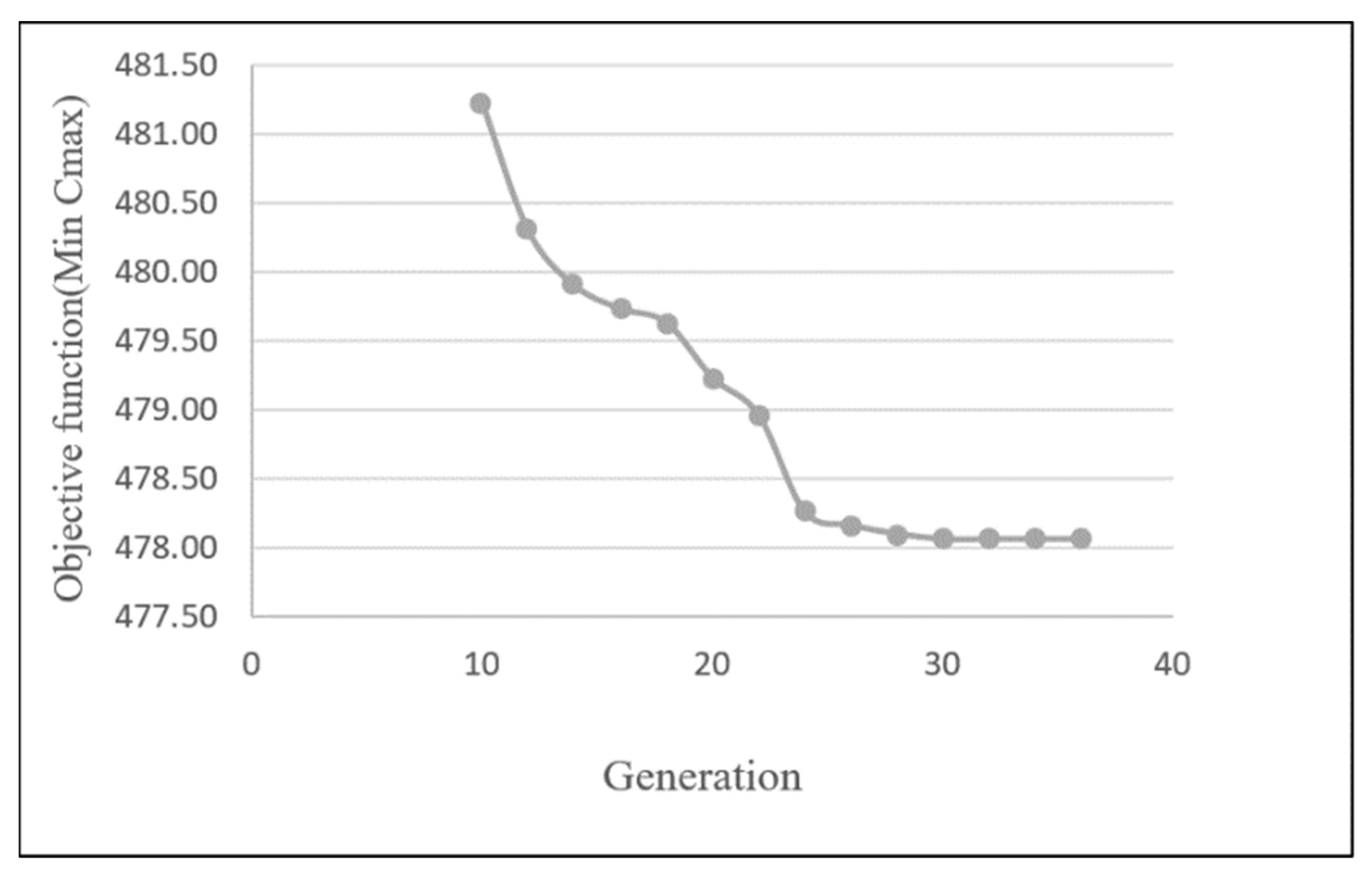
4.4. HGAG Algorithm Convergence

The HGAG convergence in the Cuexcomate cluster is evaluated using a medium-size instance: RFFS_SDST_60 × 4 × 4 × 25. Figure 8 shows the algorithm’s convergence curve as a function of the number of generations and the objective function, using a population size of 60 and processing one individual by cluster core. The results show constant improvement in the objective function value until generation 30, where convergence is reached.

4.5. Grid Efficacy

Figure 9 shows the experimental studies results considering different population sizes, which evolve with 30 generations. This Figure shows the average of 30 tests for each variation in population size, until reaching a size of 70 individuals: 60 in the Cuexcomate cluster, and 10 in the Texcal cluster. It is observed that as the size of the population increases, the quality of the solution improves. The grid impacts the solutions’ quality by using a more significant number of cooperative processes distributed throughout it.

• Process cooperation in HGAG

To perform an analysis on the cooperation of the processes in the grid, the following elements are used: 5 RFFS_SDST_ {20, 40, 60, 80, 140} test instances, six groups of cores (5, 10, 15, 30, 60, 120) and eight population sizes (5, 10, 15, 30, 60, 120, 240, 480). 30 tests are carried out by each of the following combinations of population sizes and number of cores: (5,5), (10,10), (20,20), (30,30), (60,60), (120,120), (240,120), (480,120). Each group of cores is distinguished by being closer together in an attempt to avoid bottlenecks in the grid. Two populations show core overload (240 and 480) since they must be distributed over 120 cores.

• Process cooperation in small instances

Table 7. RFFS_SDST_20 × 4 × 4 × 25 results.

RFFS_SDST_20 × 4 × 4 × 25
P	N	Np	Cmax Average	t, s Average	Best
5	5	24	481.43	361	478
10	10	12	479.67	363	472
15	15	8	479.17	364	476
30	30	4	477.70	364	473
60	60	2	476.23	366	473
120	120	1	475.10	415	471
240	120	1	473.80	1087	469

shows the results for the RFFS_SDST_20 × 4 × 4 × 25 instance. In this table, P is the number of processes, N is the number of cores, Np is the number of cores, Cmax is the mean of the 30 tests, t is the average time of the tests, and best the best makespan obtained. It is observed that the best result is obtained when an overload of processes is done and the population increases twice, from 120 to 240 individuals. This behavior is due to the algorithm conducting more exploration and exploitation of the solution space. However, the algorithm’s execution time practically increases more than double (since the processes’ communications increase) when compared to running 120 processes. In the other tests presented in Table 7, the number of individuals remains at 120.

Table 8. RFFS_SDST_40 × 4 × 4 × 25 results.

RFFS_SDST_20 × 4 × 4 × 25
P	N	Np	Cmax Average	t, s Average	Best
5	5	24	1631	1631	664
10	10	12	1696	1696	659
15	15	8	1747	1747	656
30	30	4	660.87	1664	655
60	60	2	659.30	1708	655
120	120	1	657.97	1996	654
240	120	1	656.73	4857	649

presents the results for the RFFS_SDST_40 × 4 × 4 × 25 instance. 30 runs are carried out in this test. Again, a similar behavior to the previous example is observed: the best result is obtained when an overload of processes is done. The population increases from 120 to 240 individuals, but the execution time increases more than double for the version with 120 individuals.

• Process cooperation in medium instances

Table 9. RFFS_SDST_60 × 4 × 4 × 25 results.

RFFS_SDST_60 × 4 × 4 × 25
P	N	Np	Cmax Average	t, s Average	Best
5	5	24	943.00	3889	937
10	10	12	940.27	3890	932
15	15	8	941.13	3988	934
30	30	4	939.37	3968	933
60	60	2	937.53	4047	932
120	120	1	935.73	4076	930
240	120	1	934.37	7953	927

shows the cooperation results obtained for the RFFS_SDST_60 × 4 × 4 × 25 instance. This table shows that the best result is obtained when using 240 processes and shows that the average of the 30 makespan tests and the best value found improves steadily from 15 processes, in the order 15, 30, 60, 120, 240.

Table 10. RFFS_SDST_80 × 4 × 4 × 25 results.

RFFS_SDST_80 × 4 × 4 × 25
P	N	Np	Cmax Average	t, s Average	Best
5	5	24	1282	6521	1273
10	10	12	1279	6480	1272
15	15	8	1278	6606	1270
30	30	4	1275	6618	1269
60	60	2	1274	6715	1266
120	120	1	1272	6803	1264
240	120	1	1271	13,299	1263

shows the cooperation results obtained for the RFFS_SDST_80 × 4 × 4 × 25 instance. This table shows that the best result is obtained using 240 processes and that the makespan average and the best value of the 30 tests constantly improve from five processes in the following order: 5, 10, 15, 30, 60, 120, 240. It is also observed that the execution time is close to 4 h for the case of 240 processes.

• Process cooperation in large instances

Table 11. RFFS_SDST_80 × 4 × 4 × 25 results.

RFFS_SDST_140 × 4 × 4 × 25
P	N	Np	Cmax Average	t, s Average	Best
5	5	24	2033.3	18,921	2022
10	10	12	2028.1	19,189	2015
15	15	8	2028.0	19,621	2016
30	30	4	2024.9	19,888	2016
60	60	2	2022.4	20,159	2013
120	120	1	2010.9	20,382	2013
240	120	1	2018.6	38,727	2013

shows the cooperation results obtained for the RFFS_SDST_140 × 4 × 4 × 25 instance. The best result is obtained when using 120 processes, which indicates that if the processes are increased for a large problem, the HGAG will begin to show deficiencies in its performance. This may be due to the fact that the local search generates repeated searches in the solution space. This problem could be avoided if a tabu search is implemented in the HGAG. It is observed that the makespan average and the best value of the 30 tests constantly improve from 10 processes, in the order of 10, 15, 30, 60, and 120. It is also observed that the execution time is close to 6 h for 120 processes.

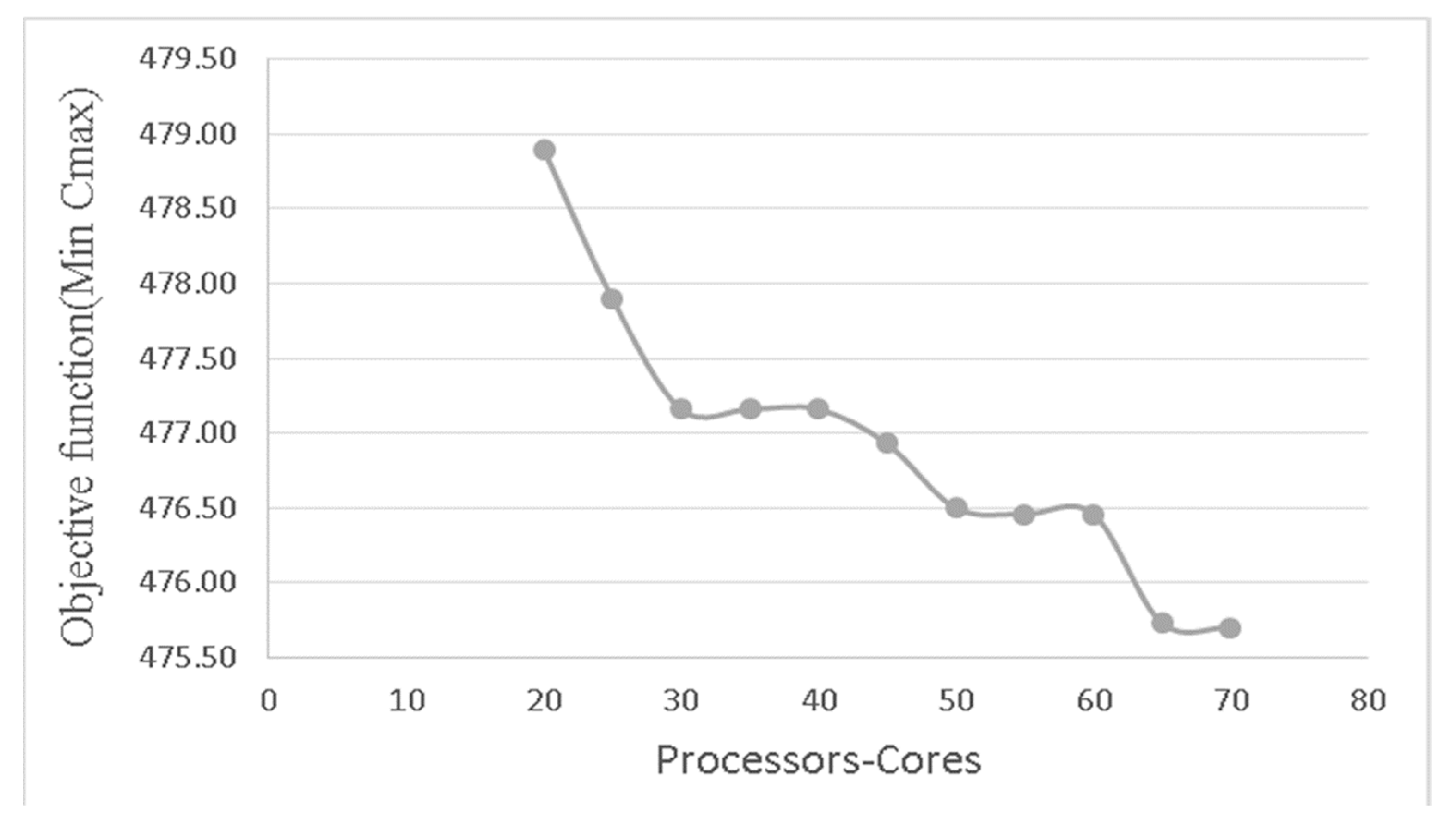
4.6. HGAG Efficiency on the Grid

Speedup evaluation

Figure 10 shows the speedup obtained in the evaluation of the RFFS_SDST_80 × 4 × 4 × 25 problem. The average efficiency of the processors’ usage is 93% when using 10, 30, 60, and 120 processes. The remaining 7% represents the non-parallelizable HGAG portion and the communications overhead. This overhead corresponds to the time used to send and receive solutions, leaving out the MPI typical synchronization times, the overload of external processes, and the Linux operating system’s communication services. When the number of processes increases, it is observed that the real speedup moves away from the ideal speedup. This behavior is due to the communications overhead increment since the algorithm data usage increases when the number of processes increases.

Evaluation of the communications overload on the Grid

The computational grid overhead is calculated based on the maximum bandwidth provided by the communication between clusters, which is 15 Mb/s. The Grid Morelos infrastructure allows two-way communication since messages can be sent and received simultaneously (upload and download). Therefore, the total bidirectional bandwidth can reach 30 Mb/s. The communication overhead is evaluated for the RFFS_SDST_80 × 4 × 4 × 25 problem, using 120 processes distributed over 120 cores and using the virtual private network joining the two clusters.

First, experimental tests of sending and returning bit packets between both clusters are carried out. The packet sizes range from 64 to 67,108,864 bits in order to evaluate the time it takes to send them. For example, the send and return time of a 64-bit packet is 750 microseconds, which is equivalent to 0.163 Mb/s. The results of these tests are described in

Table 12. Round Trip Time (RTT) evaluation in the Morelos Grid.

[fj@cuexcomate ~]$ mpiexec –ppn 1 –np 2 ./ping I am process 0 of 2 running on :cuexcomate I am process 1 of 2 running on :texcal Smaller posible measurable time ~0.953674 usecs (Microseconds)
Bits (RTT)	Time usecs	Transfer Rate Mb/sec
64	750	0.163
128	717	0.341
256	768	0.636
512	809	1.207
1024	912	2.142
2048	1128	3.463
4096	1574	4.963
8192	2471	6.323
16384	3564	8.769
32768	5917	10.563
65536	10230	12.219
131072	18921	13.213
262144	36294	13.776
524288	71130	14.059
1048576	140704	14.214
2097152	279734	14.299
4194304	559525	14.298
8388608	1115870	14.339
16777216	2354889	13.589
33554432	4748298	13.479
67108864	9321278	13.732

.

For calculating the overhead that HGAG presents when solving the RFFS_SDST_80 × 4 × 4 × 25 instance with 120 processes distributed over 120 cores in the Grid, it is necessary to determine the number of bits of a solution represented by an individual in the algorithm. The instance comprises 80 jobs, which must be executed in series on four stages, each with four identical parallel machines. The number of bits of an individual is 40,960 bits, so the population’s total size is 4,915,200 bits. As the distribution of the 120 processes in the computational grid is 60 in the Cuexcomate cluster and 60 in the Texcal cluster, only half of the population travels from one cluster to another, that is, 2,457,600 bits. Table 12, shows that, for this size, the value is between the interval (2,097,152–4,194,304). By performing an interpolation with these values, a total time of 341,689 µsecs is obtained for the population size evaluated in one generation. Therefore, the total overload time for the 30 generations is 10,250,580 µsecs, that is, approximately 10.3 s. This is the time that the algorithm spends sending and receiving the slave processes’ solutions during the total algorithm execution time.

The maximum transfer rate between clusters on the grid is 15 Mbs (15,728,640 bits/s). It is understood that the optimal transfer rate to avoid bottlenecks must be less than or equal to 15,728,640 bits/s. Table 12 shows that the highest transfer rate occurs when sending packets is 8,388,608 bits (14,339 Mb/sec). Comparing this value with the 2,457,600 bits that the HGAG uses per packet, it is clear that there is no traffic congestion between clusters since the packet size sent by the HGAG only represents 29.3% of the bandwidth available to send packages between the grid clusters.

5. Conclusions

A hybrid genetic algorithm implemented in a grid environment to solve hard instances of the flexible flow shop scheduling problem with sequence-dependent setup times is described in this paper. Each offspring generated by the evolutionary operators is improved using the combination of an iterative and cooperative local-search. The evolutionary process is conducted in a master process, and the local search is performed in a set of slave processes distributed in a grid environment. The point-to-point communication between the grid nodes is through a message passing mechanism. Since the implemented algorithm uses several parameters, and their performance depends on the values used for them, a sensibility analysis to determine the more suitable values to the parameter setting is conducted. The experimental results are analyzed considering the algorithm convergence and the efficacy and efficiency of the Morelos Grid to solve the test instances. The HGAG has an efficient convergence rate since it uses almost 30 iterations to reach a near-optimal solution.

Furthermore, the use of a set of distributed nodes impacts the solution quality since each node applies a combined local search that increases the algorithm running time if implemented in one only process. Finally, the speedup evaluation indicates that 93% of the processors’ usage is applied. It is observed that traffic congestion between clusters does not exist since the packet size transmitted by the algorithm uses 29.3% of the available bandwidth. The above values indicate that (1) the implementation of the GA with hybrid local-search in the Morelos grid allows for the finding of better RFFSP solutions, and (2) the distribution of the jobs allows for the efficient usage of the computational resources, coupled with the effective use of the grid communication.

The HGAG is an artificial intelligence heuristic algorithm. The convenience of the approach used in this work involves the combination of different search forms used to more effectively explore and exploit the solutions space, applying different procedures such as searches that allow the escape of optimal local solutions (simulated annealing), local searches with cooperation between individuals (ant colony), and also the search by exploration of the space of solutions that the genetic algorithm applies through the selection and crossover operators. Finally, exploration and exploitation in the search space is expanded in a reduced time by designing the HGAG algorithm for execution in a computational grid, applying the use of more than one computational cluster, where these clusters could be geographically distant.

6. Future Works

Future directions of this work are to implement hybrid programming using GPU-parallel programming in the Morelos Grid, since each grid cluster has GPU cards. This programming scheme will implement the hybrid local-search using SA and ACS. The genetic evolutionary process will remain in the master process to take advantage of the infrastructure’s potential. These changes are intended to improve the HGAG speed up efficiency and reduce its total execution time. It is also essential to improve the search in the space for solutions by implementing new variable neighborhood structures in SA. Finally, using a multi-objective approach of the HGAG in the job shop scheduling problem can improve the generation of more compact feature schedules for benchmark problems published in the existing literature.

References

1. Blazewicz, J.; Ecker, K.H.; Pesch, E.; Schmidt, G.; Sterna, M.; Weglarz, J. Handbook on Scheduling: From Theory to Practice; Springer International Publishing: Cham, Switzerland, 2019. [Google Scholar] [CrossRef]
2. Tun, Y.K.; Kim, D.H.; Alsenwi, M.; Tran, N.H.; Han, Z.; Hong, C.S. Energy Efficient Communication and Computation Resource Slicing for eMBB and URLLC Coexistence in 5G and Beyond. IEEE Access 2020, 8, 136024–136035. [Google Scholar] [CrossRef]
3. Fu, Y.; Ding, J.; Wang, H.; Wang, J. Two-objective stochastic flow-shop scheduling with deteriorating and learning effect in Industry 4.0-based manufacturing system. Appl. Soft. Comput. 2018, 68, 847–855. [Google Scholar] [CrossRef]
4. Lewandowski, R.; Olszewska, J.I. Automated task scheduling for automotive industry. In Proceedings of the 2020 IEEE 24th International Conference on Intelligent Engineering Systems (INES), Reykjavík, Iceland, 8–10 July 2020; pp. 159–164. [Google Scholar]
5. Fikar, C.; Hirsch, P. Home health care routing and scheduling: A review. Comput. Oper. Res. 2017, 77, 86–95. [Google Scholar]
6. Wang, H.; Gong, J.; Zhuang, Y.; Shen, H.; Lach, J. Healthedge: Task scheduling for edge computing with health mergency and human behavior consideration in smart homes. In Proceedings of the 2017 IEEE International Conference on Big Data (Big Data), Boston, MA, USA, 11–14 December 2017; pp. 1213–1222. [Google Scholar]
7. Jamroen, C.; Komkum, P.; Fongkerd, C.; Krongpha, W. An Intelligent Irrigation Scheduling System Using Low-Cost Wireless Sensor Network Toward Sustainable and Precision Agriculture. IEEE Access 2020, 8, 172756–172769. [Google Scholar] [CrossRef]
8. Demirović, E.; Stuckey, P.J. Constraint programming for high school timetabling: A scheduling-based model with hot starts. In Proceedings of the International Conference on the Integration of Constraint Programming, Artificial Intelligence, and Operations Research, Delft, The Netherlands, 26–29 June 2018; Springer: Cham, Switzerland; pp. 135–152. [Google Scholar]
9. Ullman, J.D. NP-complete scheduling problems. J. Comput. Syst. Sci. 1975, 10, 384–393. [Google Scholar] [CrossRef] [Green Version]
10. Garey, M.R.; Johnson, D.S.; Sethi, R. The complexity of flowshop and job shop scheduling. Math. Oper. Res. 1976, 1, 117–129. [Google Scholar] [CrossRef]
11. Brucker, P. Scheduling Algorithms, 2nd ed.; Springer Science & Business Media: Berlin/Germany, Heidelberg, 2004. [Google Scholar]
12. Miyata, H.H.; Nagano, M.S. The blocking flow shop scheduling problem: A comprehensive and conceptual review. Expert Syst. Appl. 2019, 137, 130–156. [Google Scholar] [CrossRef]
13. Allahverdi, A. A survey of scheduling problems with no-wait in process. Eur. J. Oper. Res. 2016, 255, 665–686. [Google Scholar] [CrossRef]
14. Filho, M.G.; de Fátima Morais, M.; Boiko TJ, P.; Miyata, H.H.; Varolo FW, R. Scheduling in flow shop with sequence-dependent setup times: Literature review and analysis. Int. J. Bus. Innov. Res. 2013, 7, 466–486. [Google Scholar] [CrossRef]
15. Pinedo, M. Scheduling Theory, Algorithms, and Systems, 3rd ed.; Prentice-Hall: Englewood Cliffs, NJ, USA, 1995. [Google Scholar]
16. Kaighobadi, M.; Venkatesh, K. Flexible Manufacturing Systems: An Overview. Int. J. Oper. Prod. Manag. 1994, 14, 26–49. [Google Scholar] [CrossRef]
17. Jungwattanakit, J.; Reodecha, M.; Chaovalitwongse, P.; Werner, F. Algorithms for flexible flow shop problems with unrelated parallel machines, setup times, and dual criteria. Int. J. Adv. Manuf. Technol. 2008, 37, 354–370. [Google Scholar] [CrossRef]
18. Ramezanian, R.; Sanami, S.F.; Nikabadi, M.S. A simultaneous planning of production and scheduling operations in flexible flow shops: Case study of tile industry. Int. J. Adv. Manuf. Technol. 2017, 88, 2389–2403. [Google Scholar] [CrossRef]
19. Peng, K.; Pan, Q.K.; Wang, L.; Deng, X.; Li, C.; Gao, L. Iterated local search for steelmaking-refining-continuous casting scheduling problem. In Proceedings of the 2019 IEEE 15th International Conference on Automation Science and Engineering (CASE), Vancouver, BC, Canada, 22–26 August 2019; pp. 567–572. [Google Scholar]
20. Sankaran, V. A Particle Swarm Optimization Using Random Keys for Flexible Flow Shop Scheduling Problems with Sequence Dependent Setup Times. Master’s Thesis, Clemson University, Clemson, SC, USA, 2009. [Google Scholar]
21. Amiri, P. Discrete Particle Swarm Optimization for Flexible Flow Line Scheduling. Master’s Thesis, Clemson University, Clemson, SC, USA, 2015. [Google Scholar]
22. Wang, C.; Hsu, H.; Fu, H.; Ky, N.; Nguyen, V.T. Scheduling Flexible Flow Shop in Labeling Companies to Minimize the Makespan. Comput. Syst. Sci. Eng. 2022, 40, 17–36. [Google Scholar] [CrossRef]
23. Tavakkoli-Moghaddam, R.; Safari, J. A New Mathematical Model for Flexible Flow Lines with Blocking Processor and Sequence-Dependent Setup Time; Levner, E., Ed.; InTechOpen: London, UK, 2007; ISBN 978-3-902613-02-8. Available online: https://www.intechopen.com/chapters/624 (accessed on 15 September 2021). [CrossRef] [Green Version]
24. Cruz-Chávez, M.A. Neighborhood Generation Mechanism Applied in Simulated Annealing to Job Shop Scheduling Problems. Int. J. Syst. Sci. 2015, 46, 2673–2685. [Google Scholar] [CrossRef]
25. Araujo, L.; Cervigón, C. Algoritmos Evolutivos; Alfa-Omega: Mexico City, Mexico, 2009. [Google Scholar]
26. Pavez-Lazo, B.; Soto-Cartes, J.; Urrutia, C.; Curilem, M. Selección Determinística y Cruce Anular en Algoritmos Genéticos: Aplicación a la Planificación de Unidades Térmicas de Generación. Ingeniare 2009, 17, 175–181. [Google Scholar]
27. Richard, P.M.; Amin, M.V.; David, E.C.; Thomas, E.A. Effects of communication latency, overhead, and bandwidth in a cluster architecture. In Proceedings of the 24th Annual International Symposium on Computer Architecture ISCA, Denver, CO, USA, 1–4 June 1997; pp. 85–97. [Google Scholar]
28. Dorigo, M. Optimization, Learning and Natural Algorithms. Ph.D. Dissertation, Dipartimento di Elettronica, Politecnico di Milano, Milano, Italy, 1992. (In Italian). [Google Scholar]
29. Wardono, B.; Fathi, Y. A tabu search algorithm for the multi-stage parallel machine problem with limited buffer capacities. Eur. J. Oper. Res. 2004, 155, 380–401. [Google Scholar] [CrossRef]
30. Kirkpatrick, C. Gelatt, and M. Vecchi. Optimization by Simulated Annealing. Science 1983, 220, 671–680. [Google Scholar] [CrossRef] [PubMed]
31. Cruz-Chávez, M.A.; Juárez-Pérez, F.; Moreno Bernal, P. MiniGrid Morelos, una Sinergia Interinstitucional, Hypatia, Revista de Divulgación Científico-Tecnológica del Consejo de Ciencia y Tecnología del Estado de Morelos; No. 40, Enero/M; Pérez Sabino, S.P., Ed.; CCYTEM: Morelos, México, 2001; pp. 32–33. ISSN 2007-4735. [Google Scholar]
32. Ruiz, A.; Stutzle, T. An Iterated Greedy heuristic for the sequence dependent setup times flowshop problem with makespan and weighted tardiness objectives. Eur. J. Oper. Res. 2008, 187, 1143–1159. [Google Scholar] [CrossRef]
33. Ruiz, R.; Vázquez-Rodríguez, J.A. The hybrid flow shop scheduling problem. Eur. J. Oper. Res. 2010, 205, 1–18. [Google Scholar] [CrossRef] [Green Version]
34. Instances. Available online: http://www.gridmorelos.uaem.mx/~mcruz/instances_RFFSP/. (accessed on 12 December 2021).
35. Ying, K.-C.; Lin, S.-W. Multi-heuristic desirability ant colony system heuristic for non-permutation flowshop scheduling problems. Int J. Adv. Manuf. Technol. 2007, 33, 793–802. [Google Scholar] [CrossRef]
36. Ruiz, R.; Maroto, C. A genetic algorithm for hybrid flowshops with sequence dependent setup times and machine eligibility. Eur. J. Oper. Res. 2006, 169, 781–800. [Google Scholar] [CrossRef]
Figure 1. A disjunctive graph representing a RFFSP with three jobs, three stages, and two machines by stage.
Applsci 12 00607 g001
Figure 2. One solution for the RFFSP with three jobs, three stages, and two machines by stage.
Applsci 12 00607 g002
Figure 3. Gantt diagram for the solution of the RFFSP.
Applsci 12 00607 g003
Figure 4. The HGAG in a grid environment using two clusters.
Applsci 12 00607 g004
Figure 5. Symbolic representation for an HGAG individual.
Applsci 12 00607 g005
Figure 6. Roulette-based crossover operator.
Applsci 12 00607 g006
Figure 7. Hybrid genetic algorithm in grid environment (HGAG).
Applsci 12 00607 g007
Figure 8. HGAG convergence for the RFFS_SDST_SDST_60 × 4 × 4 × 25 instance.
Applsci 12 00607 g008
Figure 9. HGAG behavior using different population sizes.
Applsci 12 00607 g009
Figure 10. Average speedup for the HGAG algorithm for RFFS_SDST_80 × 4 × 4 × 25 problem.
Applsci 12 00607 g010