
Parameter Sensitivity Analysis of SWAT Modeling in the Upper Heihe River Basin Using Four Typical Approaches

 ,
,  ,
,
Abstract
:1. Introduction
2. Data and Methods
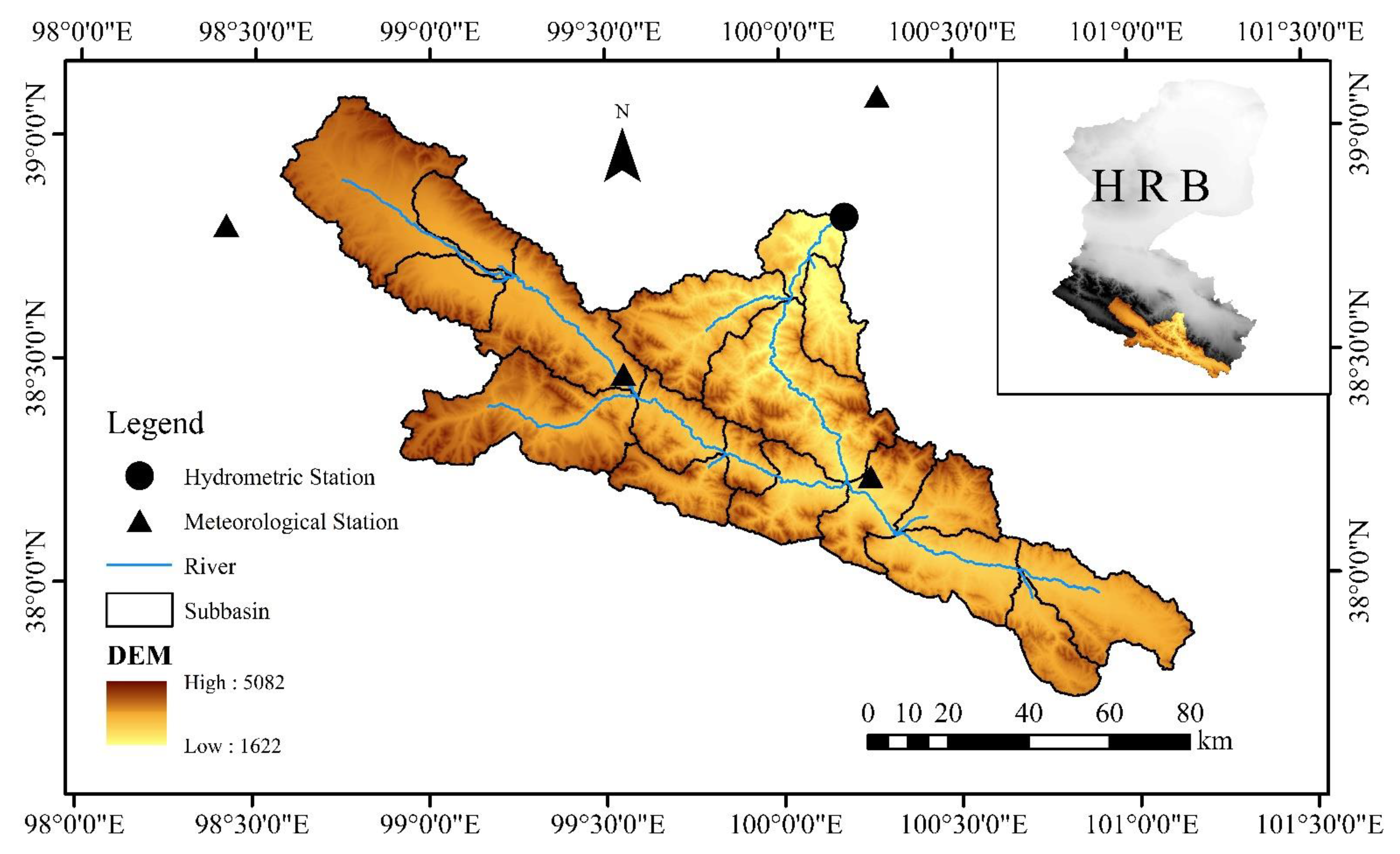
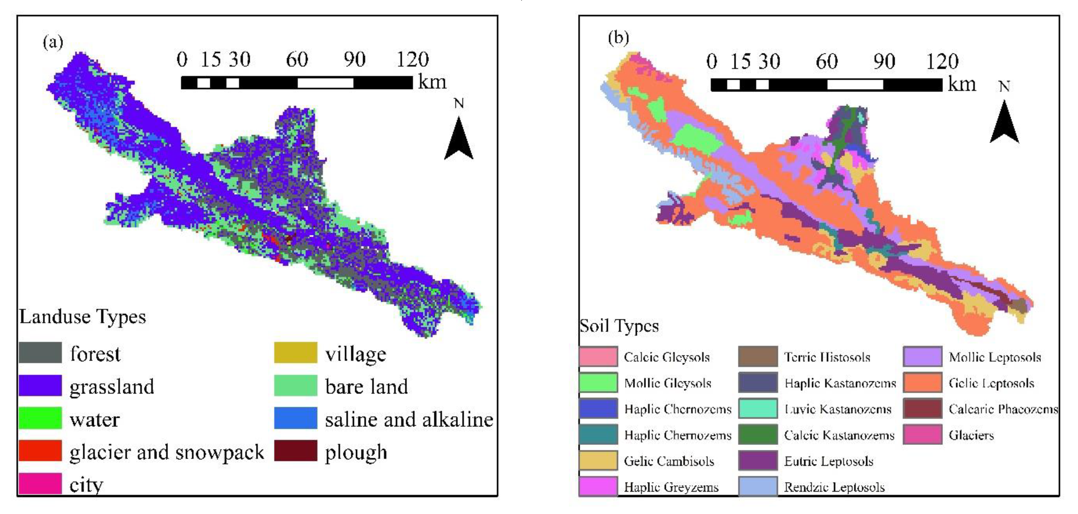
2.1. Study Area
2.2. SWAT Model
2.3. Sensitivity Analysis Methods
2.3.1. Morris Screening Method
2.3.2. Sobol Analysis Method
2.3.3. FAST Analysis Method
2.3.4. EFAST Analysis Method
3. Results
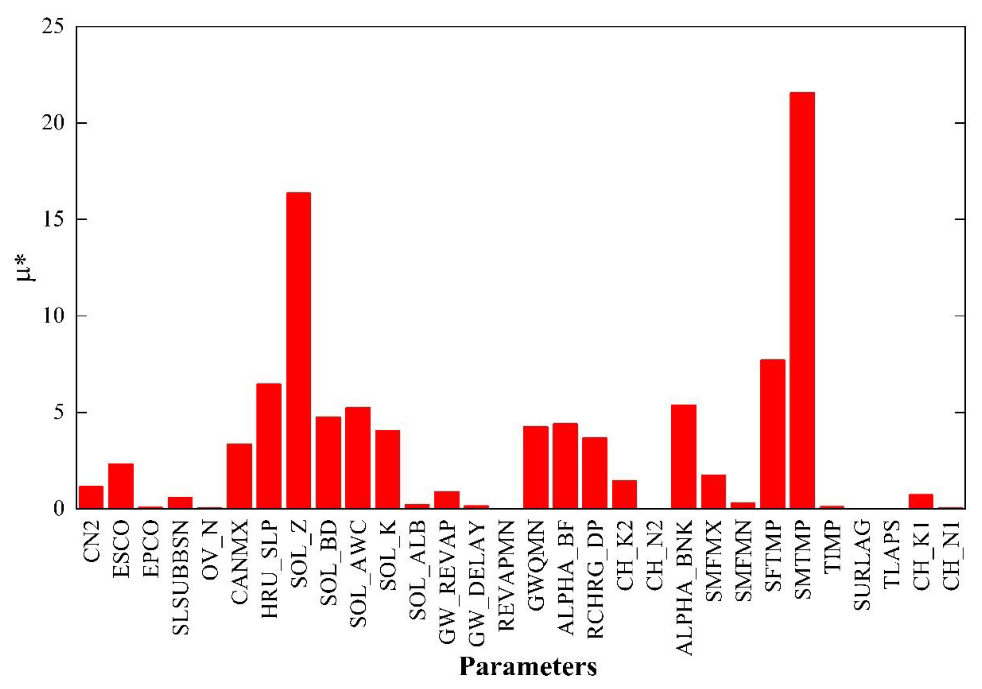
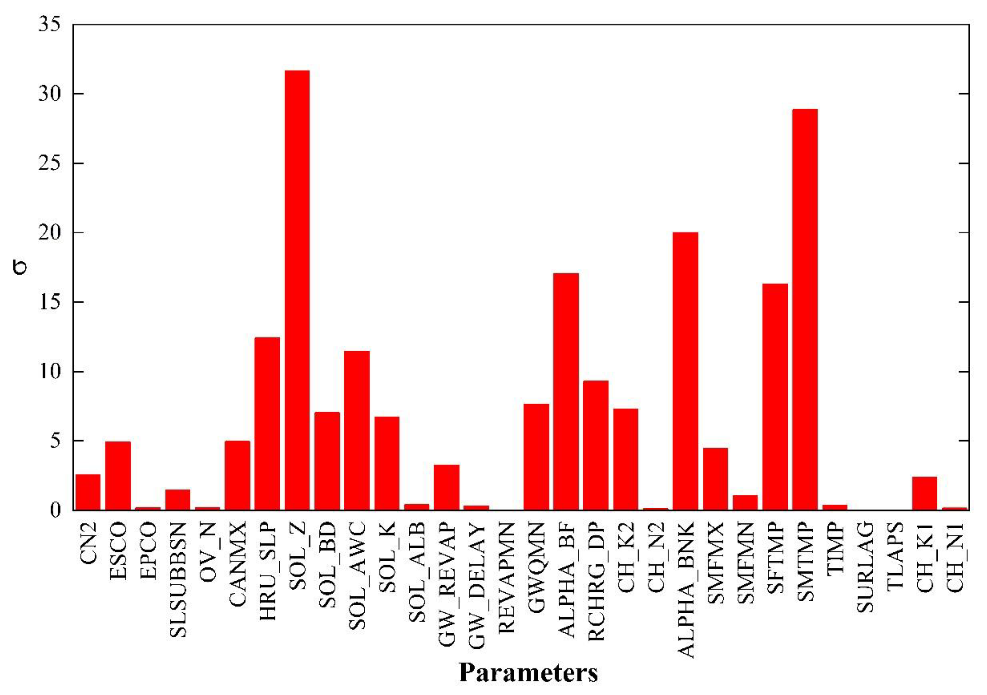
3.1. Morris Results
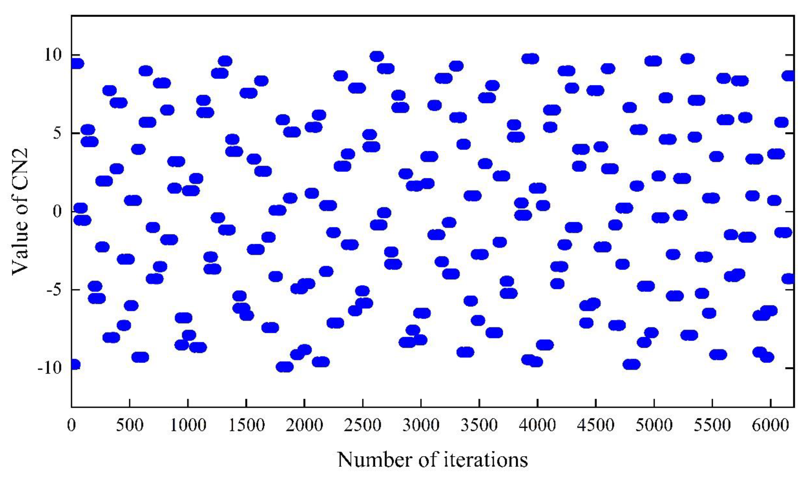
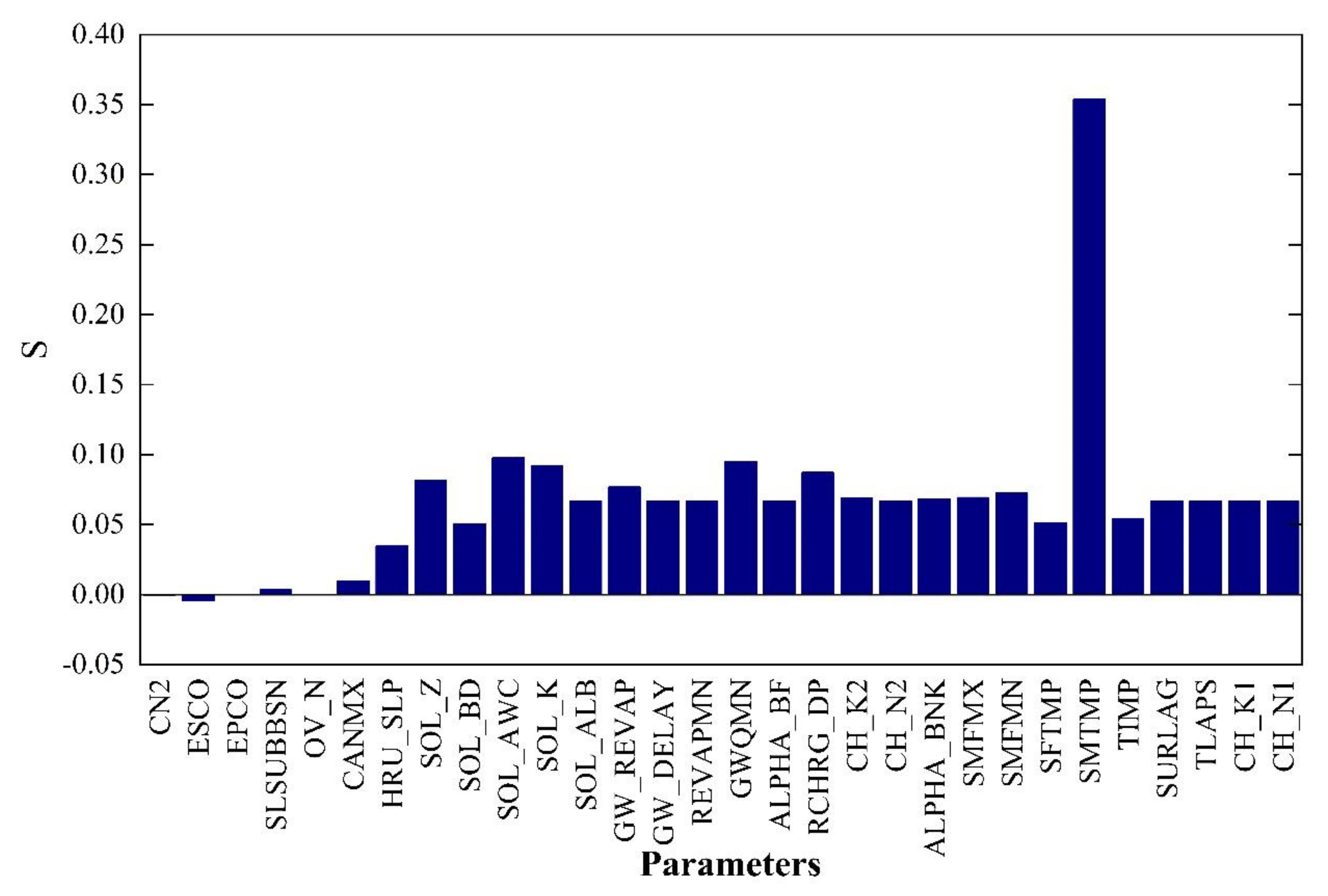
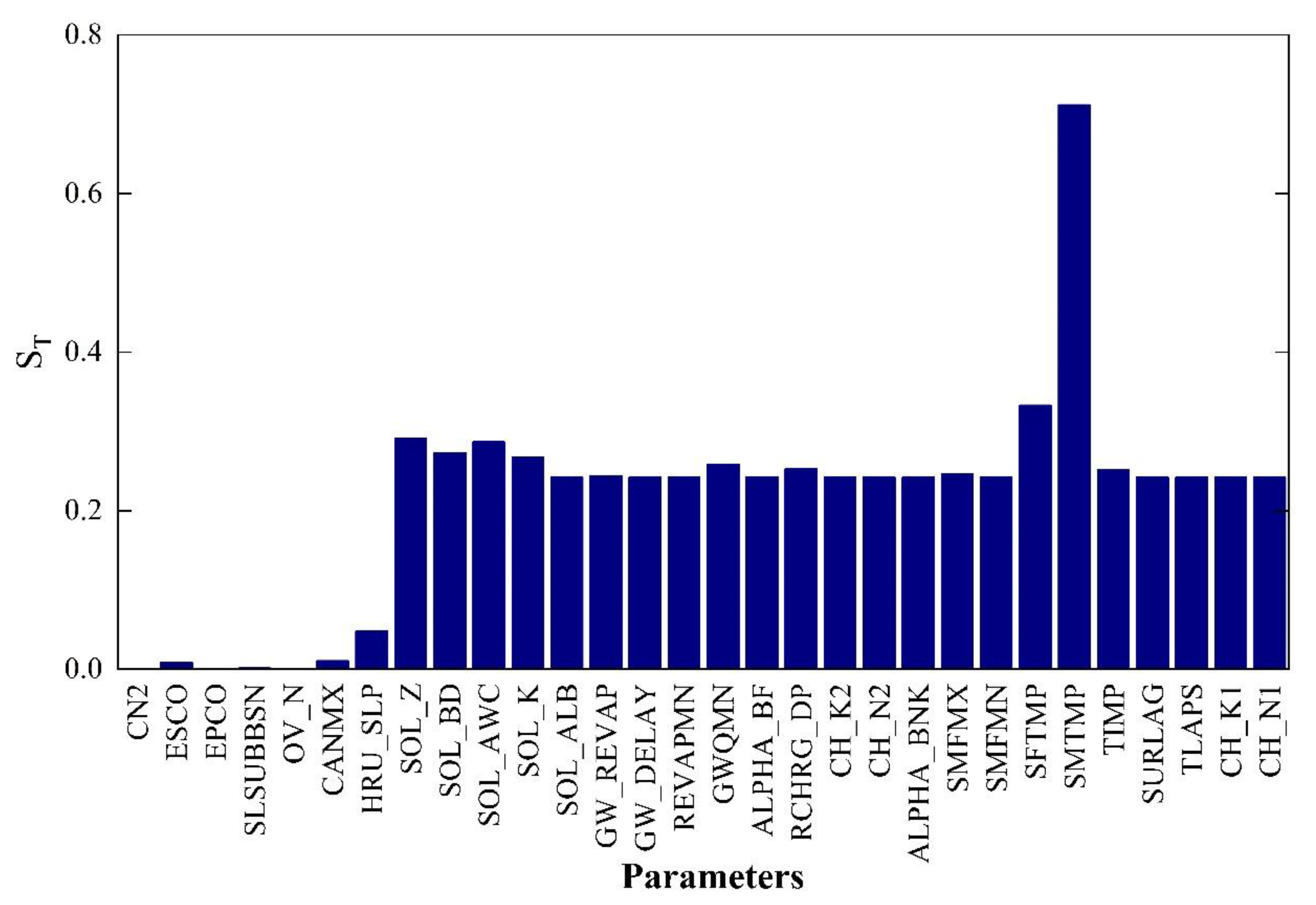
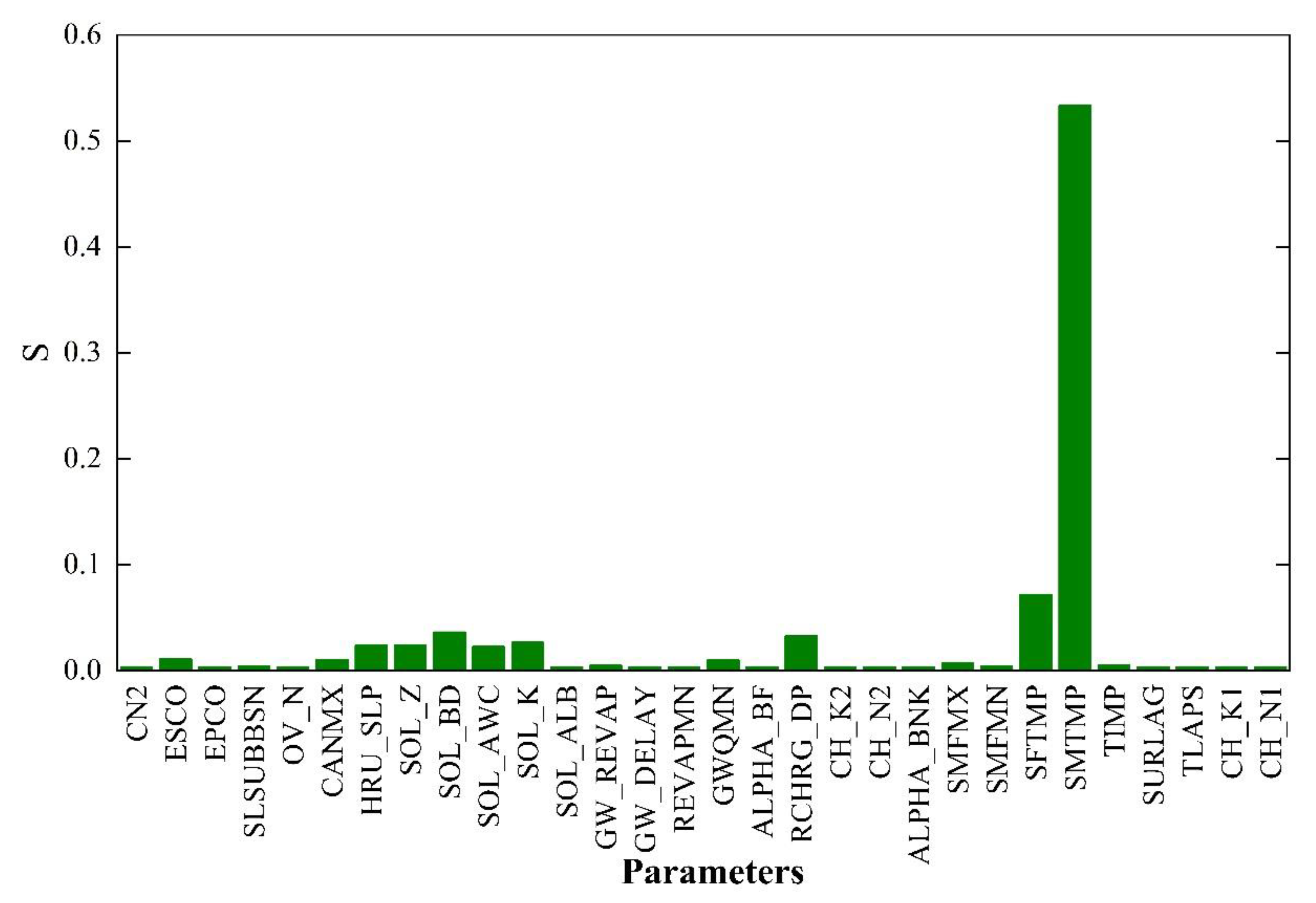
3.2. Sobol Results
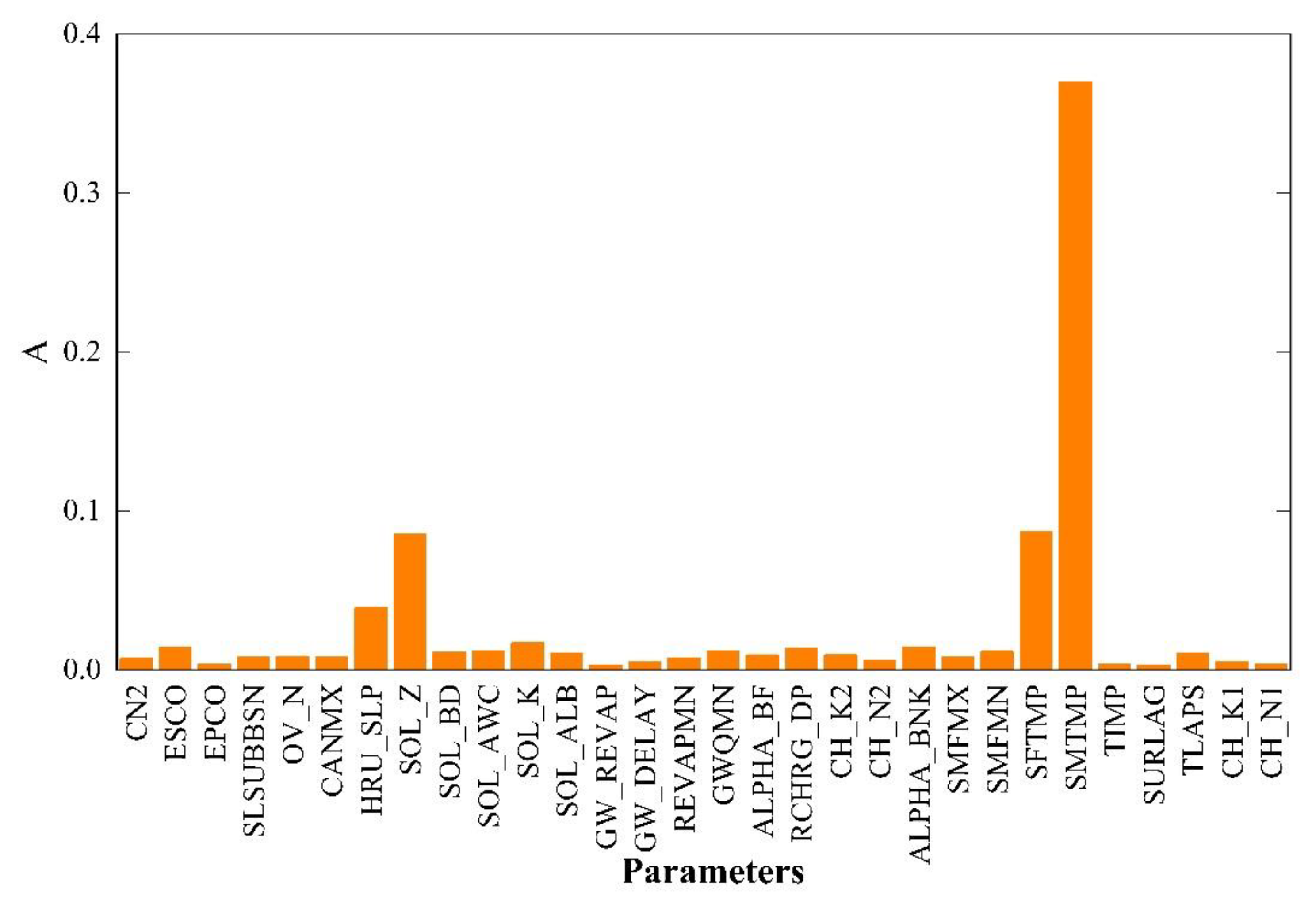
3.3. FAST Results
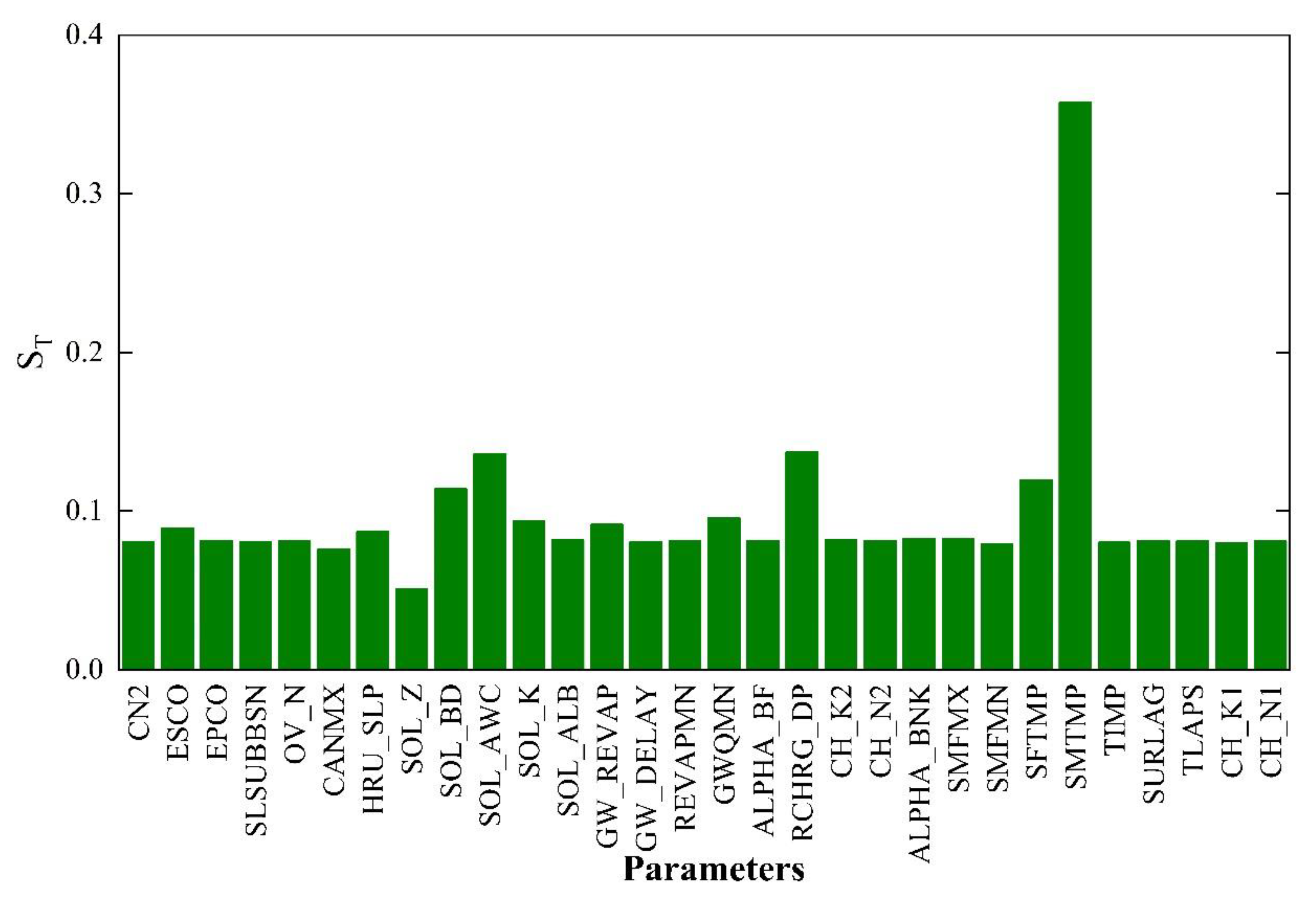
3.4. EFAST Results
3.5. Result Comparison of Different Methods
3.6. Identification of Sensitive Parameters
4. Discussion
5. Conclusions
- (1)
- Combined with the results calculated with the four parameter sensitivity analysis methods, 10 sensitive SWAT model parameters were defined: SMTMP, SOL_AWC, SFTMP, RCHRG_DP, SOL_K, SOL_Z, GWQMN, SOL_BD, ALPHA_BNK, and HRU_SLP.
- (2)
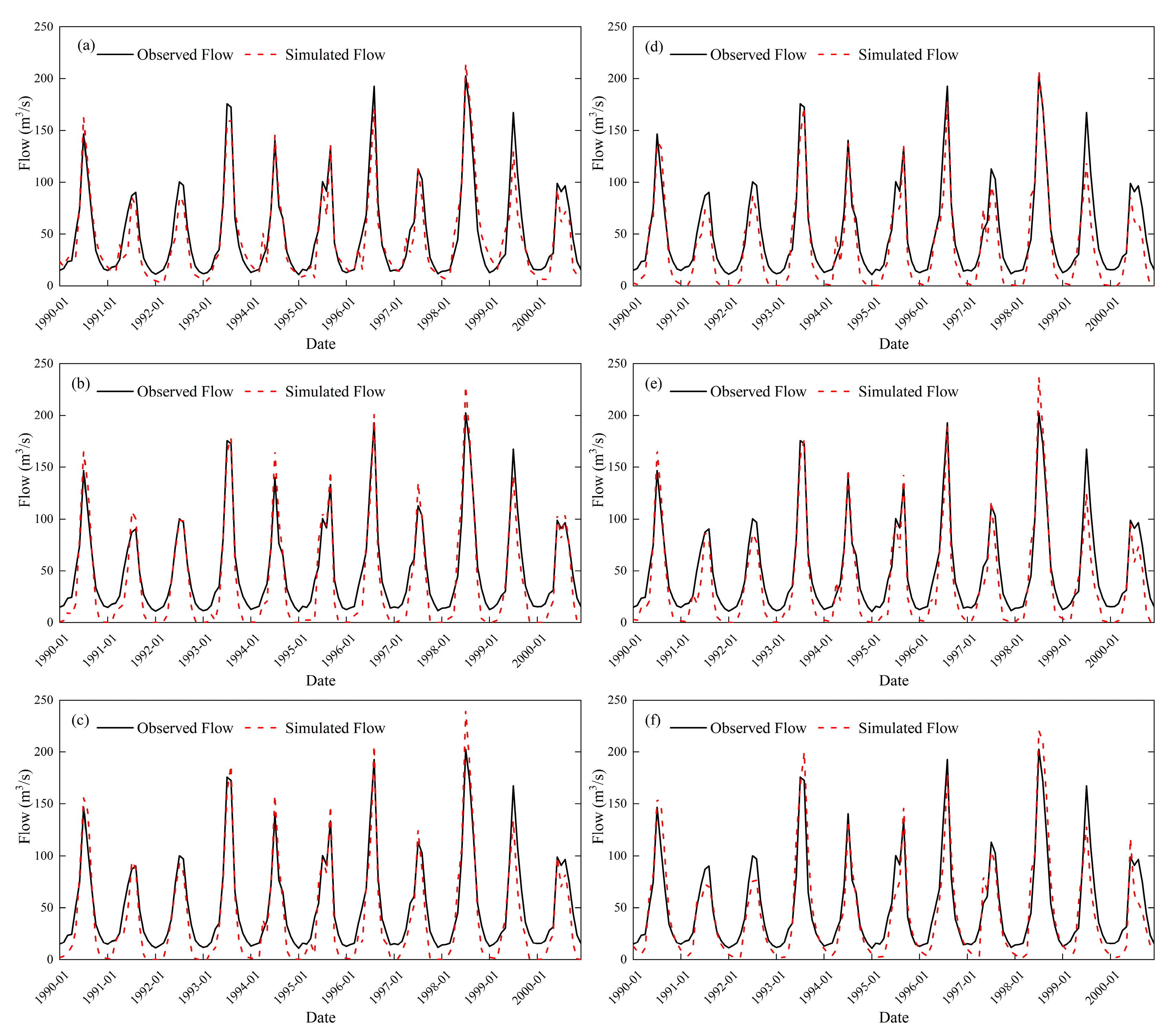
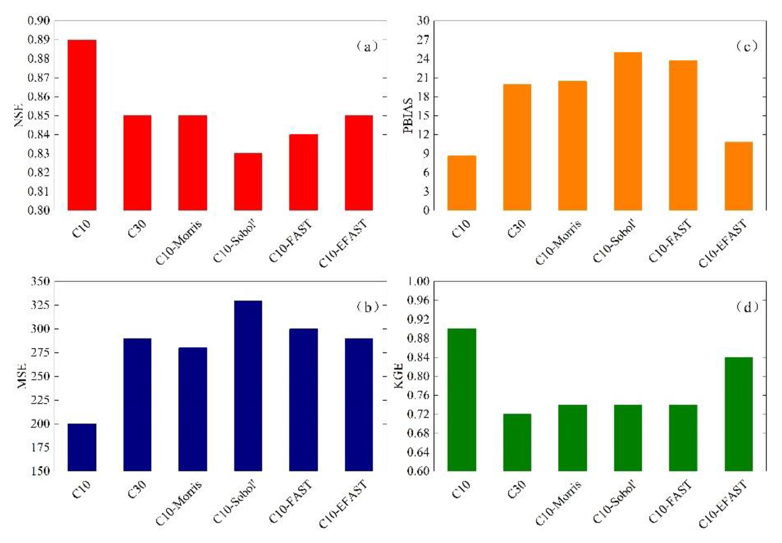
- The parameter sensitivity calculated with each analytical method was different, resulting in an apparent difference between the statistical indicators of the flow simulation value obtained by optimizing these sensitive parameters. The different sampling processes, sensitivity indices, and calculation principles of each method may be the main reasons.
- (3)
- By optimizing the most sensitive parameters combined with the results of the four methods, the NSE, MSE, PBIAS, and KGE of the flow simulation value and the measured value were 0.89, 200, 8.60, and 0.90, respectively, which were better than optimizing the sensitive parameters defined by a single method and all selected parameters. The differences in performance indicate the rationality and importance of parameter sensitivity analysis for hydrological models, and the synthesis of multiple approaches to define sensitive parameters.
Author Contributions
Funding
Institutional Review Board Statement
Informed Consent Statement
Data Availability Statement
Acknowledgments
Conflicts of Interest
References
- Song, X.; Zhan, C.; Kong, F.; Xia, J. Advances in the study of uncertainty quantification of large-scale hydrological modeling system. J. Geogr. Sci. 2011, 21, 801. [Google Scholar] [CrossRef]
- Song, X.; Zhang, J.; Zhan, C.; Xuan, Y.; Ye, M.; Xu, C. Global sensitivity analysis in hydrological modeling: Review of concepts, methods, theoretical framework, and applications. J. Hydrol. 2015, 523, 739–757. [Google Scholar] [CrossRef]
- Zhou, L.; Rasmy, M.; Takeuchi, K.; Koike, T.; Selvarajah, H.; Ao, T. Adequacy of Near Real-Time Satellite Precipitation Products in Driving Flood Discharge Simulation in the Fuji River Basin, Japan. Appl. Sci. 2021, 11, 1087. [Google Scholar] [CrossRef]
- Zhou, L.; Koike, T.; Takeuchi, K.; Rasmy, M.; Onuma, K.; Ito, H.; Selvarajah, H.; Liu, L.; Li, X.; Ao, T. A study on availability of ground observations and its impacts on bias correction of satellite precipitation products and hydrologic simulation efficiency. J. Hydrol. 2022, 610, 127595. [Google Scholar] [CrossRef]
- Mengistu, D.; Bewket, W.; Dosio, A.; Panitz, H.-J. Climate change impacts on water resources in the Upper Blue Nile (Abay) River Basin, Ethiopia. J. Hydrol. 2021, 592, 125614. [Google Scholar] [CrossRef]
- Sreedevi, S.; Eldho, T.I. A two-stage sensitivity analysis for parameter identification and calibration of a physically-based distributed model in a river basin. Hydrol. Sci. J. 2019, 64, 701–719. [Google Scholar] [CrossRef]
- Kabir, T.; Pokhrel, Y.; Felfelani, F. On the Precipitation-Induced Uncertainties in Process-Based Hydrological Modeling in the Mekong River Basin. Water Resour. Res. 2022, 58, e2021WR030828. [Google Scholar] [CrossRef]
- Faramarzi, M.; Srinivasan, R.; Iravani, M.; Bladon, K.D.; Abbaspour, K.C.; Zehnder, A.J.B.; Goss, G.G. Setting up a hydrological model of Alberta: Data discrimination analyses prior to calibration. Environ. Model. Softw. 2015, 74, 48–65. [Google Scholar] [CrossRef]
- Ehlers, L.B.; Sonnenborg, T.O.; Refsgaard, J.C. Observational and predictive uncertainties for multiple variables in a spatially distributed hydrological model. Hydrol. Process. 2019, 33, 833–848. [Google Scholar] [CrossRef]
- Liu, L.; Zhou, L.; Li, X.; Chen, T.; Ao, T. Screening and Optimizing the Sensitive Parameters of BTOPMC Model Based on UQ-PyL Software: Case Study of a Flood Event in the Fuji River Basin, Japan. J. Hydrol. Eng. 2020, 25, 05020030. [Google Scholar] [CrossRef]
- Shin, M.-J.; Jung, Y. Using a global sensitivity analysis to estimate the appropriate length of calibration period in the presence of high hydrological model uncertainty. J. Hydrol. 2022, 607, 127546. [Google Scholar] [CrossRef]
- Zhu, Y.; Liu, L.; Qin, F.; Zhou, L.; Zhang, X.; Chen, T.; Li, X.; Ao, T. Application of the Regression-Augmented Regionalization Approach for BTOP Model in Ungauged Basins. Water 2021, 13, 2294. [Google Scholar] [CrossRef]
- Chen, L.; Chen, S.; Li, S.; Shen, Z. Temporal and spatial scaling effects of parameter sensitivity in relation to non-point source pollution simulation. J. Hydrol. 2019, 571, 36–49. [Google Scholar] [CrossRef]
- Razavi, S.; Gupta, H.V. A new framework for comprehensive, robust, and efficient global sensitivity analysis: 1. Theory. Water Resour. Res. 2016, 52, 423–439. [Google Scholar] [CrossRef]
- Razavi, S.; Gupta, H.V. A new framework for comprehensive, robust, and efficient global sensitivity analysis: 2. Application. Water Resour. Res. 2016, 52, 440–455. [Google Scholar] [CrossRef]
- Khorashadi Zadeh, F.; Nossent, J.; Sarrazin, F.; Pianosi, F.; van Griensven, A.; Wagener, T.; Bauwens, W. Comparison of variance-based and moment-independent global sensitivity analysis approaches by application to the SWAT model. Environ. Model. Softw. 2017, 91, 210–222. [Google Scholar] [CrossRef]
- Cibin, R.; Sudheer, K.P.; Chaubey, I. Sensitivity and identifiability of stream flow generation parameters of the SWAT model. Hydrol. Process. 2010, 24, 1133–1148. [Google Scholar] [CrossRef]
- Song, X.; Zhan, C.; Xia, J. Integration of a statistical emulator approach with the SCE-UA method for parameter optimization of a hydrological model. Chin. Sci. Bull. 2012, 57, 3397–3403. [Google Scholar] [CrossRef]
- Wu, Q.; Liu, S.; Cai, Y.; Li, X.; Jiang, Y. Improvement of hydrological model calibration by selecting multiple parameter ranges. Hydrol. Earth Syst. Sci. 2017, 21, 393–407. [Google Scholar] [CrossRef]
- Liu, L.; Ao, T.; Zhou, L.; Takeuchi, K.; Gusyev, M.; Zhang, X.; Wang, W.; Ren, Y. Comprehensive evaluation of parameter importance and optimization based on the integrated sensitivity analysis system: A case study of the BTOP model in the upper Min River Basin, China. J. Hydrol. 2022, 610, 127819. [Google Scholar] [CrossRef]
- Morris, M.D. Factorial Sampling Plans for Preliminary Computational Experiments. Technometrics 1991, 33, 161–174. [Google Scholar] [CrossRef]
- Zhan, C.-s.; Song, X.-m.; Xia, J.; Tong, C. An efficient integrated approach for global sensitivity analysis of hydrological model parameters. Environ. Model. Softw. 2013, 41, 39–52. [Google Scholar] [CrossRef]
- Sobol, I. Sensitivity analysis for non linear mathematical model. Math. Modell. Comput. Exp. 1993, 1, 407–414. [Google Scholar]
- Cukier, R.I.; Schaibly, J.H.; Shuler, K.E. Study of the sensitivity of coupled reaction systems to uncertainties in rate coefficients. III. Analysis of the approximations. J. Chem. Phys. 1975, 63, 1140–1149. [Google Scholar] [CrossRef]
- Cukier, R.I.; Levine, H.B.; Shuler, K.E. Nonlinear sensitivity analysis of multiparameter model systems. J. Comput. Phys. 1978, 26, 1–42. [Google Scholar] [CrossRef]
- Cukier, R.I.; Fortuin, C.M.; Shuler, K.E.; Petschek, A.G.; Schaibly, J.H. Study of the sensitivity of coupled reaction systems to uncertainties in rate coefficients. I Theory. J. Chem. Phys. 1973, 59, 3873–3878. [Google Scholar] [CrossRef]
- Saltelli, A.; Chan, K.; Scott, E.M. Sensitivity Analysis; Wiley: New York, NY, USA, 2000; Volume 134. [Google Scholar]
- Houle, E.S.; Livneh, B.; Kasprzyk, J.R. Exploring snow model parameter sensitivity using Sobol’ variance decomposition. Environ. Model. Softw. 2017, 89, 144–158. [Google Scholar] [CrossRef]
- Linhoss, A.; Muñoz-Carpena, R.; Kiker, G.; Hughes, D. Hydrologic Modeling, Uncertainty, and Sensitivity in the Okavango Basin: Insights for Scenario Assessment. J. Hydrol. Eng. 2013, 18, 1767–1778. [Google Scholar] [CrossRef]
- Li, P.; Ren, L. Evaluating the effects of limited irrigation on crop water productivity and reducing deep groundwater exploitation in the North China Plain using an agro-hydrological model: I. Parameter sensitivity analysis, calibration and model validation. J. Hydrol. 2019, 574, 497–516. [Google Scholar] [CrossRef]
- Rajib, M.A.; Merwade, V.; Yu, Z. Multi-objective calibration of a hydrologic model using spatially distributed remotely sensed/in-situ soil moisture. J. Hydrol. 2016, 536, 192–207. [Google Scholar] [CrossRef]
- Gu, P.; Wu, Y.; Liu, G.; Xia, C.; Wang, G.; Xia, J.; Chen, K.; Huang, X.; Li, D. Application of meteorological element combination-driven SWAT model based on meteorological datasets in alpine basin. Water Supply 2021, 22, 3307–3324. [Google Scholar] [CrossRef]
- Jaberzadeh, M.; Saremi, A.; Ghorbanizadeh Kharazi, H.; Babazadeh, H. SWAT and IHACRES models for the simulation of rainfall-runoff of Dez watershed. Clim. Dyn. 2022. [Google Scholar] [CrossRef]
- Linh, V.T.; Tram, V.N.Q.; Dung, H.M.; Phuong, D.N.D.; Liem, N.D.; Nguyen, L.D.; Yin, C.; Kortun, A.; Loi, N.K. Meteorological and Hydrological Drought Assessment for Dong Nai River Basin, Vietnam under Climate Change. Mob. Netw. Appl. 2021, 26, 1788–1800. [Google Scholar] [CrossRef]
- Ahmadi, M.; Ascough, J.C.; DeJonge, K.C.; Arabi, M. Multisite-multivariable sensitivity analysis of distributed watershed models: Enhancing the perceptions from computationally frugal methods. Ecol. Model. 2014, 279, 54–67. [Google Scholar] [CrossRef]
- Shen, Z.; Hong, Q.; Yu, H.; Liu, R. Parameter uncertainty analysis of the non-point source pollution in the Daning River watershed of the Three Gorges Reservoir Region, China. Sci. Total Environ. 2008, 405, 195–205. [Google Scholar] [CrossRef]
- Huo, A.; Huang, Z.; Cheng, Y.; Van Liew, M.W. Comparison of two different approaches for sensitivity analysis in Heihe River basin (China). Water Supply 2019, 20, 319–327. [Google Scholar] [CrossRef]
- Singh, A.; Jha, S.K. Identification of sensitive parameters in daily and monthly hydrological simulations in small to large catchments in Central India. J. Hydrol. 2021, 601, 126632. [Google Scholar] [CrossRef]
- Sarrazin, F.; Pianosi, F.; Wagener, T. Global Sensitivity Analysis of environmental models: Convergence and validation. Environ. Model. Softw. 2016, 79, 135–152. [Google Scholar] [CrossRef]
- Fan, Z. Dynamic Patterns of the Vertical Distribution of Vegetation in Heihe River Basin since the 1980s. Forests 2021, 12, 1496. [Google Scholar] [CrossRef]
- Yang, L.; Feng, Q.; Yin, Z.; Deo, R.C.; Wen, X.; Si, J.; Liu, W. Regional hydrology heterogeneity and the response to climate and land surface changes in arid alpine basin, northwest China. Catena 2020, 187, 104345. [Google Scholar] [CrossRef]
- Li, X.; Zhang, L.; Zheng, Y.; Yang, D.; Wu, F.; Tian, Y.; Han, F.; Gao, B.; Li, H.; Zhang, Y.; et al. Novel hybrid coupling of ecohydrology and socioeconomy at river basin scale: A watershed system model for the Heihe River basin. Environ. Model. Softw. 2021, 141, 105058. [Google Scholar] [CrossRef]
- Wang, H.; Li, X.; Xiao, J.; Ma, M. Evapotranspiration components and water use efficiency from desert to alpine ecosystems in drylands. Agric. For. Meteorol. 2021, 298–299, 108283. [Google Scholar] [CrossRef]
- Han, C.; Zhang, B.; Chen, H.; Wei, Z.; Liu, Y. Spatially distributed crop model based on remote sensing. Agric. Water Manage. 2019, 218, 165–173. [Google Scholar] [CrossRef]
- Liu, S.; Li, X.; Xu, Z.; Che, T.; Xiao, Q.; Ma, M.; Liu, Q.; Jin, R.; Guo, J.; Wang, L.; et al. The Heihe Integrated Observatory Network: A Basin-Scale Land Surface Processes Observatory in China. Vadose Zone J. 2018, 17, 180072. [Google Scholar] [CrossRef]
- Zhang, Y.H.; Song, X.F.; Wu, Y.Q. Use of oxygen-18 isotope to quantify flows in the upriver and middle reaches of the Heihe River, Northwestern China. Environ. Geol. 2009, 58, 645–653. [Google Scholar] [CrossRef]
- Krysanova, V.; White, M. Advances in water resources assessment with SWAT—An overview. Hydrol. Sci. J. 2015, 60, 771–783. [Google Scholar] [CrossRef]
- Gassman, P.W.; Sadeghi, A.M.; Srinivasan, R. Applications of the SWAT Model Special Section: Overview and Insights. J. Environ. Qual. 2014, 43, 1–8. [Google Scholar] [CrossRef]
- Francesconi, W.; Srinivasan, R.; Pérez-Miñana, E.; Willcock, S.P.; Quintero, M. Using the Soil and Water Assessment Tool (SWAT) to model ecosystem services: A systematic review. J. Hydrol. 2016, 535, 625–636. [Google Scholar] [CrossRef]
- Touseef, M.; Chen, L.; Masud, T.; Khan, A.; Yang, K.; Shahzad, A.; Wajid Ijaz, M.; Wang, Y. Assessment of the Future Climate Change Projections on Streamflow Hydrology and Water Availability over Upper Xijiang River Basin, China. Appl. Sci. 2020, 10, 3671. [Google Scholar] [CrossRef]
- Hwang, S.; Jun, S.-M.; Song, J.-H.; Kim, K.; Kim, H.; Kang, M.-S. Application of the SWAT-EFDC Linkage Model for Assessing Water Quality Management in an Estuarine Reservoir Separated by Levees. Appl. Sci. 2021, 11, 3911. [Google Scholar] [CrossRef]
- Nachtergaele, F.O.; Velthuizen, H.v.; Verelst, L.; Batjes, N.H.; Dijkshoorn, J.A.; Engelen, V.W.P.v.; Fischer, G.; Jones, A.; Montanarella, L.; Petri, M.; et al. Harmonized World Soil Database (Version 1.0); Food and Agric Organization of the UN (FAO): Rome, Italy, 2008. [Google Scholar]
- Koo, H.; Chen, M.; Jakeman, A.J.; Zhang, F. A global sensitivity analysis approach for identifying critical sources of uncertainty in non-identifiable, spatially distributed environmental models: A holistic analysis applied to SWAT for input datasets and model parameters. Environ. Model. Softw. 2020, 127, 104676. [Google Scholar] [CrossRef]
- Koo, H.; Iwanaga, T.; Croke, B.F.W.; Jakeman, A.J.; Yang, J.; Wang, H.-H.; Sun, X.; Lü, G.; Li, X.; Yue, T.; et al. Position paper: Sensitivity analysis of spatially distributed environmental models- a pragmatic framework for the exploration of uncertainty sources. Environ. Model. Softw. 2020, 134, 104857. [Google Scholar] [CrossRef]
- Campolongo, F.; Cariboni, J.; Saltelli, A. An effective screening design for sensitivity analysis of large models. Environ. Model. Softw. 2007, 22, 1509–1518. [Google Scholar] [CrossRef]
- Homma, T.; Saltelli, A. Importance measures in global sensitivity analysis of nonlinear models. Reliab. Eng. Syst. Saf. 1996, 52, 1–17. [Google Scholar] [CrossRef]
- Iman, R.L.; Hora, S.C. A Robust Measure of Uncertainty Importance for Use in Fault Tree System Analysis. Risk Anal. 1990, 10, 401–406. [Google Scholar] [CrossRef]
- Gao, S.; Li, Z.; Zhang, P.; Chen, Q.; Zeng, J.; Zhao, C.; Liu, C.; Zheng, Z. Global Sensitivity Analysis of the MEMLS Model for Retrieving Snow Water Equivalent. IEEE Trans. Geosci. Remote Sens. 2022, 60, 1–15. [Google Scholar] [CrossRef]
- Zhang, R.; Chen, T.; Chi, D. Global Sensitivity Analysis of the Standardized Precipitation Evapotranspiration Index at Different Time Scales in Jilin Province, China. Sustainability 2020, 12, 1713. [Google Scholar] [CrossRef]
- Yang, J. Convergence and uncertainty analyses in Monte-Carlo based sensitivity analysis. Environ. Model. Softw. 2011, 26, 444–457. [Google Scholar] [CrossRef]
- Saltelli, A.; Annoni, P.; Azzini, I.; Campolongo, F.; Ratto, M.; Tarantola, S. Variance based sensitivity analysis of model output. Design and estimator for the total sensitivity index. Comput. Phys. Commun. 2010, 181, 259–270. [Google Scholar] [CrossRef]
- Nazari-Sharabian, M.; Taheriyoun, M.; Karakouzian, M. Sensitivity analysis of the DEM resolution and effective parameters of runoff yield in the SWAT model: A case study. J. Water Supply Res. Technol. 2019, 69, 39–54. [Google Scholar] [CrossRef]
- Gull, S.; Shah, S.R. Hydrological modeling for streamflow and sediment yield simulation using the SWAT model in a forest-dominated watershed of north-eastern Himalayas of Kashmir Valley, India. J. Hydroinf. 2022, jh2022042. [Google Scholar] [CrossRef]
- Wu, L.; Liu, X.; Chen, J.; Yu, Y.; Ma, X. Overcoming equifinality: Time-varying analysis of sensitivity and identifiability of SWAT runoff and sediment parameters in an arid and semiarid watershed. Environ. Sci. Pollut. Res. 2022, 29, 31631–31645. [Google Scholar] [CrossRef] [PubMed]
- Setti, S.; Barik, K.K.; Merz, B.; Agarwal, A.; Rathinasamy, M. Investigating the impact of calibration timescales on streamflow simulation, parameter sensitivity and model performance for Indian catchments. Hydrol. Sci. J. 2022, 67, 661–675. [Google Scholar] [CrossRef]


| Parameters | Description | Hydrologic Process |
|---|---|---|
| CN2 | Initial SCS runoff curve number for moisture condition II | Surface runoff processes |
| SURLAG | Surface runoff lag coefficient | |
| ESCO | Surface runoff lag coefficient | Potential and actual evapotranspiration processes |
| EPCO | Plant uptake compensation factor | |
| CANMX | Maximal canopy storage (mm H2O) | |
| SOL_ALB | Moist soil albedo | |
| SOL_Z | Depth from the soil surface to the bottom of the layer (mm) | Soil water processes |
| SOL_BD | Moist bulk density (Mg/m3 or g/cm3) | |
| SOL_AWC | Available water capacity of the soil layer (mm H2O/mm soil) | |
| SOL_K | Saturated hydraulic conductivity (mm/h) | |
| GW_REVAP | Groundwater evapotranspiration coefficient | Groundwater processes |
| GW_DELAY | The delay time | |
| REVAPMN | Threshold depth of water in the shallow aquifer for evapotranspiration or percolation to the deep aquifer to occur (mm H2O) | |
| GWQMN | Threshold depth of water in the shallow aquifer required for return flow to occur (mm H2O) | |
| ALPHA_BF | Baseflow alpha factor (1/day) | |
| RCHRG_DP | Deep aquifer percolation fraction | |
| CH_K2 | Effective hydraulic conductivity in main channel alluvium (mm/h) | Channel water routing processes |
| CH_N2 | Manning’s “n” value for the main channel | |
| ALPHA_BNK | Baseflow alpha factor for bank storage (days) | |
| SMFMX | Melt factor for snow on 21 June (mm H2O/°C/day) | Snow processes |
| SMFMN | Melt factor for snow on 21 December (mm H2O/°C/day) | |
| SFTMP | Snowfall temperature (°C) | |
| SMTMP | Snow melt base temperature (°C) | |
| TIMP | Snowpack temperature lag factor. | |
| SLSUBBSN | Surface runoff lag coefficient | Time of concentration processes |
| OV_N | Manning’s “n” value for overland flow | |
| CH_N1 | Manning’s “n” value for the tributary channels | |
| CH_K1 | Effective hydraulic conductivity in tributary channel alluvium (mm/h) | Transmission losses from surface runoff Processes |
| HRU_SLP | Average slope steepness (m/m) | Lateral flow processes |
| TLAPS | Temperature lapse rate (°C/km) | Elevation bands |
| Parameter | IE | Parameter | IE | Parameter | IE |
|---|---|---|---|---|---|
| SMTMP | 0.3578 | REVAPMN | 0.1753 | GW_REVAP | 0.1674 |
| SFTMP | 0.2814 | ALPHA_BF | 0.1753 | RCHRG_DP | 0.1661 |
| SOL_BD | 0.2226 | CH_N2 | 0.1753 | GWQMN | 0.1636 |
| SOL_Z | 0.2095 | SURLAG | 0.1753 | HRU_SLP | 0.0138 |
| TIMP | 0.1977 | TLAPS | 0.1753 | ESCO | 0.0125 |
| SOL_AWC | 0.189 | CH_N1 | 0.1753 | CANMX | 0.001 |
| SMFMX | 0.1768 | GW_DELAY | 0.1752 | CN2 | 0.0004 |
| SOL_K | 0.1764 | ALPHA_BNK | 0.1739 | EPCO | 0 |
| CH_K1 | 0.1754 | CH_K2 | 0.1735 | OV_N | 0 |
| SOL_ALB | 0.1753 | SMFMN | 0.1704 | SLSUBBSN | −0.0019 |
| Ranking | Morris | Sobol’ | FAST | EFAST |
|---|---|---|---|---|
| 1 | SOL_Z | SMTMP | SMTMP | SMTMP |
| 2 | SMTMP | SOL_AWC | SFTMP | RCHRG_DP |
| 3 | ALPHA_BNK | SOL_Z | SOL_Z | SFTMP |
| 4 | SFTMP | SOL_K | HRU_SLP | SOL_BD |
| 5 | HRU_SLP | GWQMN | SOL_K | SOL_AWC |
| 6 | ALPHA_BF | RCHRG_DP | ESCO | SOL_K |
| 7 | SOL_AWC | GW_REVAP | ALPHA_BNK | HRU_SLP |
| 8 | SOL_BD | SMFMX | RCHRG_DP | GWQMN |
| 9 | GWQMN | SMFMN | SOL_AWC | ESCO |
| 10 | RCHRG_DP | CH_K2 | GWQMN | GW_REVAP |
| Ranking | Parameter | Value Range | Optimal Value | Ranking | Parameter | Value Range | Optimal Value |
|---|---|---|---|---|---|---|---|
| 1 | SMTMP | (−5, 5) | −4.65 | 6 | SOL_Z | (0, 1000) | 625 |
| 2 | SOL_AWC | (0, 1) | 0.075 | 7 | GWQMN | (0, 1000) | 535 |
| 3 | SFTMP | (−5, 5) | 2.05 | 8 | SOL_BD | (0.9, 2.5) | 1.116 |
| 4 | RCHRG_DP | (0, 1) | 0.945 | 9 | ALPHA_BNK | (0, 1) | 0.695 |
| 5 | SOL_K | (0, 100) | 5.5 | 10 | HRU_SLP | (0, 1) | 0.845 |
Publisher’s Note: MDPI stays neutral with regard to jurisdictional claims in published maps and institutional affiliations. |
© 2022 by the authors. Licensee MDPI, Basel, Switzerland. This article is an open access article distributed under the terms and conditions of the Creative Commons Attribution (CC BY) license (https://creativecommons.org/licenses/by/4.0/).
Share and Cite
Xiang, X.; Ao, T.; Xiao, Q.; Li, X.; Zhou, L.; Chen, Y.; Bi, Y.; Guo, J. Parameter Sensitivity Analysis of SWAT Modeling in the Upper Heihe River Basin Using Four Typical Approaches. Appl. Sci. 2022, 12, 9862. https://doi.org/10.3390/app12199862
Xiang X, Ao T, Xiao Q, Li X, Zhou L, Chen Y, Bi Y, Guo J. Parameter Sensitivity Analysis of SWAT Modeling in the Upper Heihe River Basin Using Four Typical Approaches. Applied Sciences. 2022; 12(19):9862. https://doi.org/10.3390/app12199862
Chicago/Turabian StyleXiang, Xin, Tianqi Ao, Qintai Xiao, Xiaodong Li, Li Zhou, Yao Chen, Yao Bi, and Jingyu Guo. 2022. "Parameter Sensitivity Analysis of SWAT Modeling in the Upper Heihe River Basin Using Four Typical Approaches" Applied Sciences 12, no. 19: 9862. https://doi.org/10.3390/app12199862