Article

Unified Modeling and Analysis of Vibration Energy Harvesters under Inertial Loads and Prescribed Displacements

1
RISE Research Institutes of Sweden AB, 411 33 Gothenburg, Sweden
2
Department of Microtechnology and Nanoscience, Chalmers University of Technology, 412 58 Gothenburg, Sweden
3
Department of Mathematics and Mathematical Statistics, Umeå University, 901 87 Umeå, Sweden
*
Author to whom correspondence should be addressed.
Appl. Sci. 2022, 12(19), 9815; https://doi.org/10.3390/app12199815
Submission received: 30 August 2022 / Revised: 23 September 2022 / Accepted: 26 September 2022 / Published: 29 September 2022
(This article belongs to the Special Issue Energy Harvesting by Smart Materials)

Abstract

:
In this paper, we extend the optimization analysis found in the current literature for single-degree-of-freedom vibrational energy harvesters. We numerically derive and analyze the optimization conditions based on unified expressions for piezoelectric and electromagnetic energy harvesters. Our contribution lies in the detailed analysis and comparison of both resonant and anti-resonant states while fully including the effect of intrinsic resistance. We include both the case of excitation by inertial load and prescribed displacement, as the latter has not been elaborated on in the previous literature and provides new insights. We perform a general analysis but also consider typical values of applied piezoelectric and electromagnetic energy harvesters. Our results improve upon previous similar comparative studies by providing new and useful insights regarding optimal load, load power and power input to output efficiency. Our analysis shows an exponential increase in the critical mechanical quality factor due to the resistive loss coefficient. We find that the ratio of mechanical quality factor to resistive loss coefficient, at resonance, increases drastically close to the theoretical maximum for load power. Under the same optimization conditions, an equivalent conclusion can be drawn regarding efficiency. We find that the efficiency at anti-resonance behaves differently and is equal to or larger than the efficiency at resonance. We also show that the optimal load coefficient at resonance has a significant dependence on the mechanical quality factor only when the resistive loss coefficient is large. Our comparison of excitation types supports the previous literature, in a simple and intuitive way, regarding optimal load by impedance matching and power output efficiency. Our modeling and exploration of new parameter spaces provide an improved tool to aid the development of new harvester prototypes.

1. Introduction

Vibrational energy harvesters (VEHs) based on piezoelectric [1,2,3] or inductive [4,5,6] transduction have been frequently modeled in the previous literature, typically as lumped second-order mass–spring–damper systems. Power output at resonance and anti-resonance, power optimal load and efficiency are typically included in these analyses. The efficiency is typically defined as the ratio of input mechanical energy to output electrical energy, which is equivalent to the ratio of input power to output power [1]. Resonance and anti-resonance refer to the case of coupled oscillators being either in phase (resonance) or out of phase (anti-resonance). Resonance occurs when the electrical damping is at its smallest, i.e., short-circuit conditions for a piezoelectric energy harvester (PEH) and open-circuit conditions for an electromagnetic energy harvester (EMEH). This corresponds to the natural frequency of the mechanical structure. Anti-resonance occurs when the electrical damping is at its largest, i.e., open-circuit conditions for the PEH and short circuit for the EMEH.
Essential parameters in these models are mechanical quality factor, ratio of excitation frequency to natural frequency, intrinsic impedance and resistance, load resistance and the electromechanical coupling coefficient. The latter is defined by the ratio of electrostatic (PEH) or electromagnetic (EMEH) energy to mechanical energy. There is a critical value of the effective electromechanical coupling coefficient, which is determined by the mechanical quality factor, at which the output power reaches a theoretical maximum, and an anti-resonant peak starts to emerge, as derived by Liao et al. [3].
The lumped mechanics of a PEH or EMEH can be modeled in a unified way, assuming they are both systems with linear stiffness and damping. This has been exploited by [7,8,9] to derive a general model applicable for both systems.
Arroyo et al. [8] performs a thorough derivation of a general expression for generated power, normalized by the theoretical power limit. The analysis focuses on the generated power for varying load, mechanical quality factor and effective electromechanical coupling. Optimal load coefficients are described, but the optimal frequency, normalized by the natural frequency, is simply taken to be 1, thus not addressing the case of anti-resonance. In their paper, they note that the effective electromechanical coupling and resistive loss coefficient are both large for a typical EMEH and small for a typical PEH. From their survey, they also find a few existing PEHs achieving power performances close to the theoretical limit, while the typical EMEH has room for improvement.
Wang et al. has modeled the power output for VEHs in several papers and included the harmonic case [7], cases with different types of loads, reactive and passive [10,11], and a derivation method which allows both harmonic and stochastic input to be used [12,13]. In [7], Wang et al. performs a similar analysis to that conducted by Arroyo et al. [8] (although theirs includes the aspect of harvesting efficiency) but assumes an effective coupling coefficient under the critical value, and thus the anti-resonant point is lost in the analysis. Contrary to [8], Wang et al. neglects the intrinsic resistance for the PEH/EMEH (i.e., coil and dielectric resistance), which is common practice for PEHs but is not generally applicable for an EMEH and results in incorrect optimal load resistance [6,14].
Tai et al. [15] derive separate dimensionless expressions for the average load power generated from a PEH and EMEH. Optimization here is primarily performed and analyzed relative to the electrical damping ratio and normalized excitation frequency. The case of nonnegligible intrinsic resistance is only considered for the EMEH and treated only numerically for two discrete values of the ratio of load resistance to intrinsic resistance. Their analysis deviates from the common approach in that they mainly consider the case of constant base displacement amplitude. The critical effective electromechanical coupling coefficient, as defined in [3], is only treated for the case of a PEH and only discussed regarding the optimal load resistance.
In [16], Liao et al. derive a general expression for the PEH power output using the equivalent circuit method, in which the entire system is expressed and solved in the electrical domain. The same theoretical power limit as mentioned previously is derived here and applies regardless of the interface circuit. A significant contribution of their analysis is an increased understanding of the critical electromechanical coupling coefficient and how it is affected by various interface circuits. The intrinsic resistance, and thus resistive loss coefficient, is not included in the analysis, and the characteristics of the resonant and anti-resonant solutions are not discussed.
Wang et al. and others [1,7,17] arrive at the same expression for PEH efficiency. Kunz [18] notes that previous models of PEH efficiency are lacking in a common approach to calculation. According to Kunz, the theoretical efficiency over-estimates the real scenario as the damping from air viscosity is not considered. Although the analysis by Wang et al. [7] includes efficiency, in the context of both PEHs and EMEHs, it does so under the assumption of the negligible effect from intrinsic resistance.
In this paper, we use the lumped second-order mass–spring–damper system for the mechanical domain, and the lumped element system for the electrical domain, to derive a common dimensionless expression for generated power and efficiency, valid for both PEHs and EMEHs. In order to capture all the essential VEH characteristics, our model consists of a mechanical quality factor, an effective electromechanical coupling coefficient, an excitation frequency normalized by the natural frequency and two dimensionless coefficients accounting for intrinsic resistance and load resistance, defined as the resistive loss coefficient and load coefficient. Using the same set of parameters, we derive expressions for output power and efficiency based on system excitation from both inertial load and prescribed displacement. The comparison between these two types of excitations has not been performed in the previous literature.
To show the effect of all input parameters, in a relevant and clear way, we perform a numerical investigation in the domain of the mechanical quality factor and resistive loss coefficient, under the condition of optimal excitation frequency and load resistance. The effective electromechanical coupling coefficient is also varied to examine its dependence. As there are local power optima at both resonance and anti-resonance, we characterize the model at both points. Based on typical systems parameters, we compare the EMEH and PEH in the above defined space. Such an investigation, examining and comparing system characteristics at both resonance and anti-resonance while also considering the effect from the resistive loss coefficient in a detailed way, has not been performed in the previous literature, and results in new useful insights.

2. Method

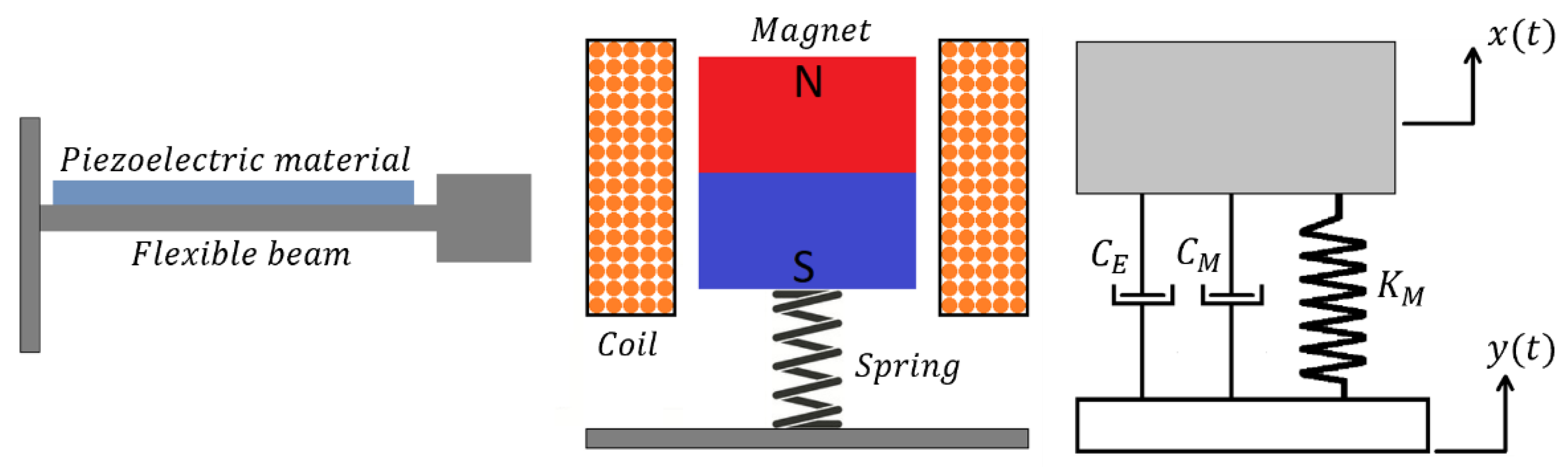
To find a common expression for PEH and EMEH power output, we use the second-order mass–spring–damper system and describe the proof mass movement of both PEHs and EMEHs, using Equation (1). Proof mass displacement is expressed as x t , m is the effective mass, C M is the total mechanical damping factor, K M is the mechanical spring constant, y t is the base displacement, and f is the damping force resulting from extracting electrical energy from the system. The corresponding free-body diagram is shown in Figure 1 (right).
m x ¨ + C M x ˙ + K M x + f = m y ¨
The electrical damping force, f , for the PEH and EMEH is given by Equation (2).
PEH :                         f = θ v EMEH :                 f = θ i
Here, v and i are the instantaneously generated voltage and current for the respective VEH. θ is a system-specific coupling factor and is a function of harvester dimensions and material properties, such as the piezoelectric coefficient or the magnetic remanence. The coupling factor relates displacement to current or voltage by:
PEH :                         θ x ˙ = i EMEH :                 θ x ˙ = v
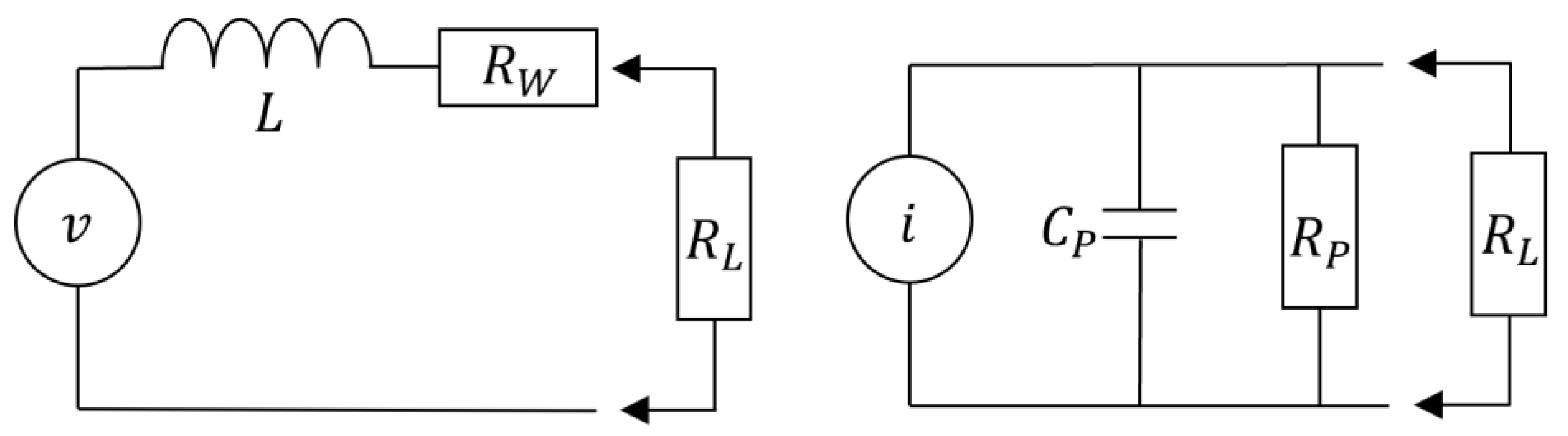
Next, we use the lumped element model in the electrical domain to express the generated power as a function of f . In Figure 2, we model the EMEH as a voltage source, v , in series with an ideal inductor, L , and winding resistance, R w . The PEH is modeled as a current source, i , in parallel with an ideal capacitance, C P , and an electric resistance, R P , due to the resistivity of the PEH. We use Kirchhoff’s first and second law to find the relationship between current and voltage in each case.
PEH :                           i = C P v ˙ + v R L + v R P EMEH :                 v = L d i d t + R w + R L i
We can use Equation (4) together with Equations (2) and (3) to express proof mass displacement velocity as a function of the electrical damping, resulting in Equation (5).
PEH :                         x ˙ = 1 θ 2 C P f ˙ + f R L + f R P EMEH :                 x ˙ = 1 θ 2 L f ˙ + R w + R L f
To find a general governing equation, we perform the variable substitutions A = 1 / R T and B = C P for the PEH and A = R T and B = L for the EMEH. R T is the total output resistance and is given by Equation (6):
PEH :                         R T = R P R L R P + R L EMEH :                 R T = R w + R L
Applying the above-defined variables to Equation (5) yields a common expression for the proof mass velocity, as given by Equation (7).
x ˙ = 1 θ 2 A f + B f ˙
The total average power, generated over the resistive components, can be derived from the RMS voltage or current as:
PEH :                         P T = A v / 2 2 EMEH :                 P T = A i / 2 2
Using Equations (2) and (8), we can arrive at a general expression for the average power:
P T = A f ^ 2 2 θ 2
As our model assumes a purely resistive load, the average load power (Equation (10)) is found by applying a resistive division term to Equation (9).
PEH :                         P = P T R P R P + R L EMEH :                 P = P T R L R W + R L
As in the previous literature [7,8], we normalize the power output by a reference power ω 2 y 0 2 m 2 / C M , where ω is angular excitation frequency and y 0 is the base displacement amplitude and use a set of dimensionless parameters according to Table 1. For a more concise power expression, we further parameterize with dimensionless parameters according to Table 2. The same variable substitution as described earlier, regarding A and B, is used in Table 1 and Table 2 where applicable.
Using Equations (1), (7), (9) and (10) and the dimensionless parameters described in Table 1 and Table 2, we can derive a unified expression for dimensionless average load power under inertial load, P ¯ I L (see derivation in Supplementary Materials).
P I L C M ω 2 y 0 2 m 2 = P ¯ I L = α β ξ C 2 1 + α 2 + β γ 2 2 ε α β γ + ε 2 1 + β γ 2
Equations (7), (9) and (10) can be used to derive the equivalent expression under prescribed displacement since x t = y t . As the effect of electric damping on proof mass displacement is negated in this case, the load power under prescribed displacement ( P P D ) can be derived in a more direct way by taking the square of the RMS voltage (for a PEH) or current (for an EMEH) acting on the load, multiplied or divided by the load resistance (see derivation in Supplementary Materials). We can express this in a unified manner using the same set of dimensionless parameters as before. For comparability with the case of inertial load, we can also extract the same reference power as mentioned previously, which results in Equation (12).
P ¯ P D = 2 ζ 2 α β ξ C γ 2 1 + β γ 2
The efficiency is defined as the average generated power by average input power [1]. For the case of inertial load, we use the input power as derived by Yang et al. (see Equation (13))
P I n = F × y ˙ = m x ¨ + y ¨ y ˙
Given the derivations in [1], this results in the average input power given by Equation (14).
P I L I n = 1 2 m x ¨ y ˙ × sin x
where x is the phase difference between x and y . In the case of prescribed displacement, there is no phase difference and x = y . We use Equation (1) together with Equation (13) to define the input power under prescribed displacement, resulting in Equation (15).
P P D I n = F × y ˙ = m x ¨ + C M x ˙ + K M x + f x ˙
In both cases, this leads to an efficiency according to Equation (16) (see derivation in Supplementary Materials).
Γ = P P I n = α β ξ C 1 + β γ 2 + α
In summary, we derive (i) the dimensionless average power generated over the load resistance, Equation (11), based on a lumped second-order mass–spring–damper system with inertial load, Equation (1), and the lumped element model, Equation (4), for both the PEH and EMEH; (ii) the dimensionless average power assuming a prescribed proof mass displacement, Equation (12), and (iii) an expression for efficiency, Equation (16), relating load power to mechanical input power, valid for both the PEH and EMEH under both inertial load and prescribed displacement. Next, we analyze these general expressions to determine the common and dual characteristics of piezoelectric and electromagnetic energy harvesters.

3. Results

3.1. Power Optimization of System under Inertial Load

The local optima for dimensionless power, in the domain of γ and ξ C , can be determined from the zeros of the corresponding partial derivatives of the power expression. One approach to finding the analytical solution to the local power optima is to first find the relation between γ and optimal load coefficient from the zeros of P ¯ / ξ C (assuming ω N and B are constants):
ξ C = γ 2 + ξ E 2 + Q η 2 ξ E + Q η 2 ε γ ε 2 + 1
By applying Equation (17) in Equation (11), we find the expression for dimensionless power under the condition of optimal load, given by Equation (18).
P ¯ I L _ O p t L o a d = Q η / 4   γ 2 ε ´ 2 + 1 ε 2 + 1 + ξ E ε 2 + 1 2 Q η + ξ E ε 2 + 1 + ξ E ε 2 + 1 + Q η
For a more concise expression, an additional parameter, ε ´ , is used in Equation (18). This additional parameter is defined by Equation (19).
ε ´ = Q γ 2 η + 1 γ
The zeros of the derivative with respect to γ , P ¯ I L _ O p t L o a d / γ , then give the local optimum γ . However, without assuming negligible ξ E , we find the analytical root derivation to be prohibitively complex, even for an analytical software tool. We therefore perform a numerical investigation to determine the model characteristics under optimal excitation frequency and load resistance. We find the locally optimal values of γ and ξ C by finding the intersections of solutions to P ¯ I L / ξ C = 0 and P ¯ I L / γ = 0 .
To compare our results with the previous literature, we can set ξ E = 0 in Equation (18) and solve for P ¯ I L _ O p t L o a d / γ = 0 , in which case we arrive at the same solutions as Liao et al. [3], under the restrictions of positive and real solutions. Under the same condition of ξ E = 0 , we also find a critical value of the effective electromechanical coupling, η c r i t = 4 ζ 1 + ζ , above which the number of real and positive solutions to P ¯ I L _ O p t L o a d / γ = 0 increases from one to three, where one solution is a local minimum. For η η c r i t there is only a single maximum.
In our continued investigation, we will use an equivalent critical value, expressed as a quality factor, given by Equation (20).
Q c r i t = 1 + 1 + η / η
Q c r i t is used in the same way as η c r i t ; i.e., for Q Q c r i t , there is only one real maximum, and for Q > Q c r i t , there are two real maxima. For the case of Q Q c r i t and ξ E = 0 , the two possible local power maxima, with respect to γ , tend toward the open-circuit ( β ,   γ 1 + η ) and closed-circuit ( β ,   γ   1 ) resonance frequencies, also called resonance and anti-resonance. In our investigation, we dub the solution tending toward resonance as γ o p t _ R , and for the solution tending toward anti-resonance, we use γ o p t _ A R . Correspondingly we use ξ C _ o p t _ R and ξ C _ o p t _ A R .
The results from our numerical investigation show that for ξ E > 0 , there still exists a critical value of Q (or equivalently, η ), above which we find three viable local optima, although it is significantly modified by the inclusion of ξ E . As we do not have the exact analytical expression for the new boundary, we perform our analysis by varying Q in factors of Q c r i t . For this reason, we introduce the parameter k , defined by Equation (21).
k = Q / Q c r i t
Figure 3 shows k c r i t as a function of ξ E at η = 0.1 ,   0.5 ,   1 ,   5 , where k c r i t is the minimum value of k required for the existence of an anti-resonant solution. We see that increasing η reduces k c r i t for a given value of ξ E .
Applying Q = Q c r i t results in a single maximum at γ = 1 + η 1 4 = 1 + 2 ζ . Applying Q = Q c r i t and γ = 1 + 2 ζ results in P ¯ I L _ O p t L o a d = 1 / 8 , i.e., the theoretical maximum load power. Liao et al. [3] show that the dimensionless power at the local optima reach a maximum of 1 / 8 for Q Q c r i t and ξ E = 0 .

3.1.1. Resonant Solution

Figure 4 shows the values for γ o p t _ R , as a function of k and ξ E , at η = 5 ,   1 ,   0.1 . The general behavior is that for k 1 , γ o p t _ R 1 , and the dependance on ξ E becomes negligible in the given range. For k 1 , γ o p t _ R tends to be below unity, inversely proportional to η , but approaches unity for ξ E 1 . For k 1 , we see the largest dependance between γ o p t _ R and ξ E , primarily in the region of ξ E 1 . For k = 1 and ξ E = 0 , we find that γ o p t _ R = 1 + 1 / Q c r i t , which is also derived in [3].
Figure 5 shows ξ C _ o p t _ R as a function of k and ξ E . For ξ E 1 , ξ C _ o p t _ R is a linear function Q with a slope proportional to η and an offset which is a linear function of ξ E . For ξ E 1 , the relation between Q and ξ C _ o p t _ R is nonlinear in the region close to k = 1 . Figure 6 shows the optimal load coefficient as a function of k for η = 5 ,   0.1 and ξ E = 0 ,   0.1 . For k = 1 , ξ E = 0 and γ o p t _ R = 1 + 1 / Q c r i t , we have ξ C _ o p t _ R = Q c r i t + 1 / Q c r i t .
Figure 7 shows the power at resonance with optimal load as a function k and ξ E . As determined in the previous literature, the maximum power over the load resistance is a factor with 1/8 of the reference power, for ξ E = 0 . Any increase in ξ E naturally leads to a reduction in the maximum power, which can be generated over the load, for a given value of Q . This effect is mitigated in systems with a large Q value.

3.1.2. Anti-Resonance Solution

Figure 8 shows the values for γ o p t _ A R , as a function of k and ξ E , at η = 5 ,   1 . For k 1 , the value of γ o p t _ A R tends towards 1 + η . Contrary to the resonant case, γ o p t _ A R has a significant dependence of ξ E even at large values of Q . As stated earlier, there is no valid solution for γ o p t _ A R at Q < k c r i t Q c r i t . For k = 1 and ξ E = 0 , we have γ o p t _ A R = 1 + 1 / Q c r i t , i.e., the resonance and anti-resonance peaks merge at k = 1 , and there is a single global optimum for γ .
Figure 9 shows ξ C _ o p t _ A R as a function of k and ξ E . Contrary to the resonant case, ξ C _ o p t _ A R has an overall nonlinear relationship to both k and ξ E and decreases with increasing k . At k = 1 and ξ E = 0 , we have ξ C _ o p t _ A R = Q c r i t + 1 / Q c r i t .
Figure 10 shows the power at anti-resonance with optimal load as a function k and ξ E . Again, the maximum power over the load resistance is a factor with 1/8 of the reference power for ξ E = 0 . Compared to the resonant case, we can see that there is a larger decrease in P ¯ I L at increasing ξ E . Contrary to the resonant case, as k is increased, ξ E has a larger negative effect on the output power.

3.2. Power Optimization of System under Prescribed Displacement

The system under prescribed displacement naturally lacks resonance (and by extension, anti-resonance). There is thus no optimal value of gamma. An optimal load coefficient can be found from the zeros of P ¯ P D / ξ C (assuming ω N and B are constants):
ξ C = γ 2 + ξ E 2
Applying Equation (22) in Equation (12), we find:
P ¯ P D _ O p t L o a d = α 2 Q γ 2
A comparative investigation with the case of inertial load can be made by setting the excitation frequency as equal for both cases. For a fair comparison, we assume the excitation frequency follows the power optimal value for the case of inertial load (see Figure 4). The corresponding power under prescribed displacement, with a power optimal load (Equation (23)), is shown in Figure 11. From Figure 4, we see that the value of γ is small when k 1 , unless ξ E 1 . As γ 2 is in the denominator of Equation (23), the value of P ¯ P D _ O p t L o a d naturally escalates in the region k 1 , ξ E < 1 . This is a result of using the reference power as normalization, which decreases with decreasing Q (or equivalently k ), while the (non-normalized) output power, P P D _ O p t L o a d , is independent of Q . A similar argument can be made for the case of anti-resonant frequencies. At resonance, the dimensionless power under prescribed displacement is generally larger than that for the case of inertial load. For anti-resonant frequencies, the dimensionless power under inertial load can be larger than that for prescribed displacement if the resistive loss coefficient is small and the mechanical quality factor is sufficiently large.

3.3. Efficiency Optimization

The derived expression for efficiency has no optimum with respect to γ and decreases at increasing γ . With regard to k and the resistive loss coefficient, the behavior is similar to that of the load power (compare Figure 12 with Figure 7), if γ and ξ C follow the power-optimized values. The maximum efficiency at resonance is in this case 50%, while Figure 13 shows a maximum efficiency slightly above 50% at anti-resonance.
The optimum load with regard to efficiency is given by Equation (24). Applying Equation (24) in Equation (16) results in Equation (25). We can see then that the expression for efficiency allows for close to 100% efficiency if ξ E is negligible and 2 γ / Q η << 1. As an example, the maximum efficiency at γ = 1 and η = 1 is approximately 86%, as seen in Figure 14.
ξ C _ o p t = γ 2 + ξ E 2 + ξ E Q η
Γ O p t L o a d = Q η 2 ξ E + Q η + 2 ξ E 2 + γ 2 + ξ E Q η

4. Discussion

The unified models, Equations (11) and (12), show the common ground of both types of energy harvesters, PEHs and EMEHs. In the space of the dimensionless parameters γ , Q , ξ E , ξ C and η , both systems are identical.
Our modeling results for inertially loaded VEH systems highlight differences in characteristics when run at resonance compared to anti-resonance. A relevant comparison can be made between these states and how the differences affect performance. This comparison is made especially relevant as the material characteristics, and the series vs. parallel circuit nature for the respective systems, lead to significantly different ranges of ξ E , η and optimal ξ C .
We highlight additional characteristics of VEHs by comparing our results from the model with inertial load to those from the model assuming prescribed displacement.
Based on applied EMEHs/PEHs from the literature, we use the typical values for Q , ξ E and η to identify which regions of the k - ξ E space typically correspond to which VEH. From this, we can use our modeling results to characterize and compare typical applied EMEH/PEH systems.

4.1. Performance Comparison of Resonant and Anti-Resonant States

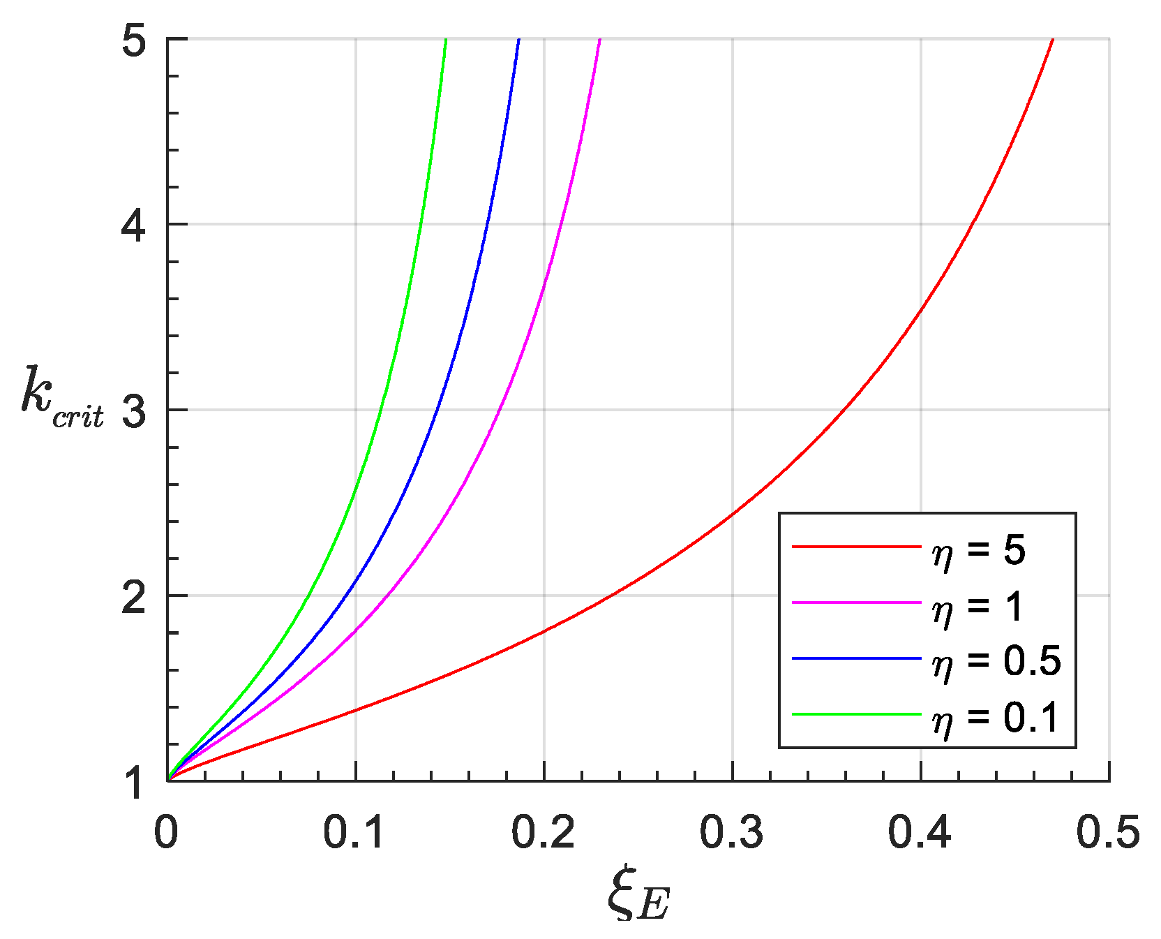
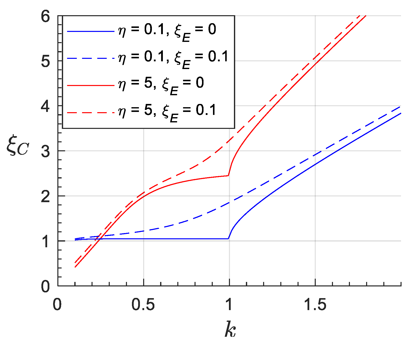
Both the resistive loss coefficient and the effective electromechanical coupling coefficient play a significant role in determining if VEH systems exhibit anti-resonance. As seen in Figure 3, η and ξ E define a critical value of Q , at which the power reaches a theoretical limit and an anti-resonant peak starts to emerge. For systems with equivalent mechanical properties, the difference in η and ξ E can thus determine if they are on opposite sides of this critical value of Q (or equivalently, k c r i t ).
Assuming we can design an arbitrary EMEH or PEH to operate either at the resonant or the anti-resonant state, the two VEH systems will benefit differently from operating under either condition. Using the results of Section 3, we can compare these states regarding the key performance parameters: output voltage, power and efficiency.
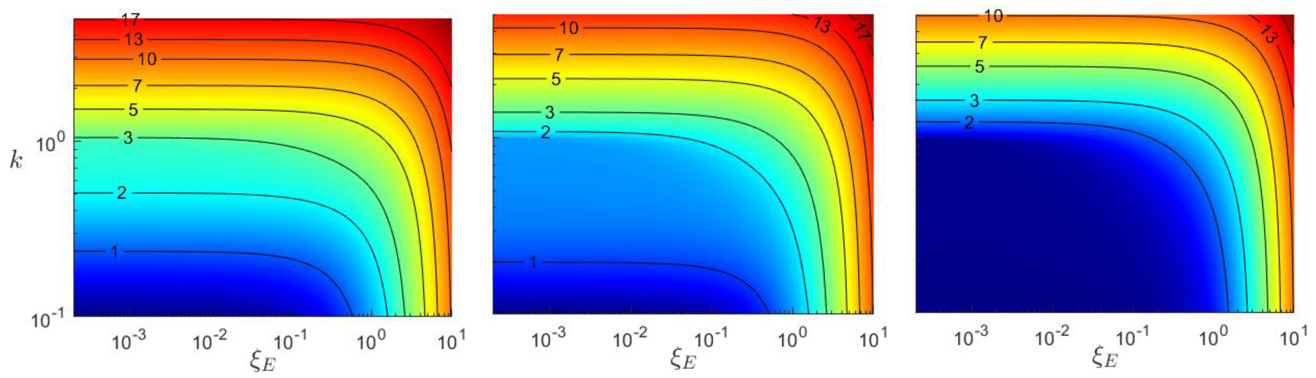
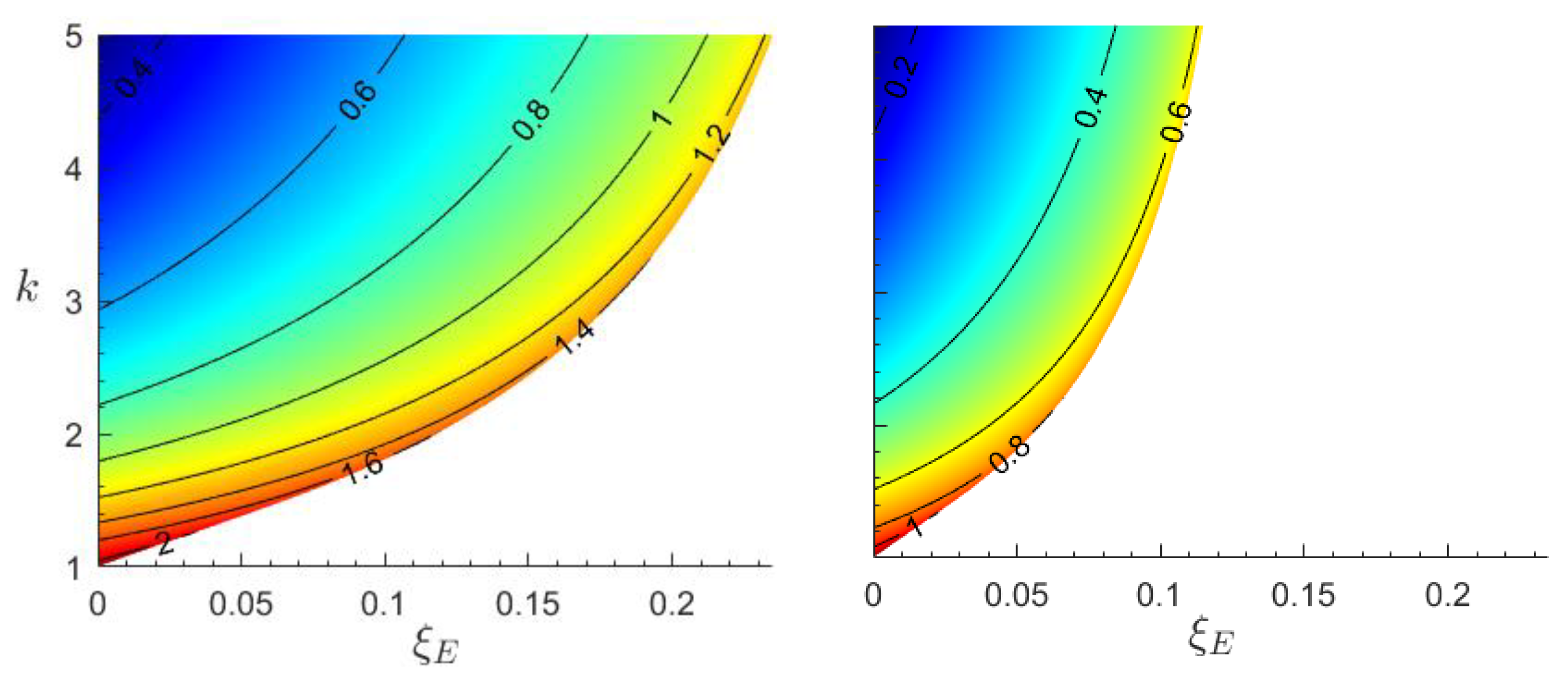
In general, a large output voltage is beneficial due to the substantial voltage drop in typical voltage rectification circuits. Due to the series nature of the EMEH circuit model, a large output voltage is obtained when ξ C is large and ξ E is small, while for a PEH, both should be small. From the results in Figure 5 and Figure 6, we can see that a system run at resonance can in general achieve large values of optimal ξ C at high k values. On the contrary, values of optimal ξ C 1 at resonance require large values of η and k 1 (see Figure 6). Only at anti-resonance (see Figure 9) can we achieve an optimal ξ C 1 at small values of η . In both cases (PEH/EMEH), an increasingly beneficial value of optimal ξ C , with regard to output voltage, is achieved at increasing k .
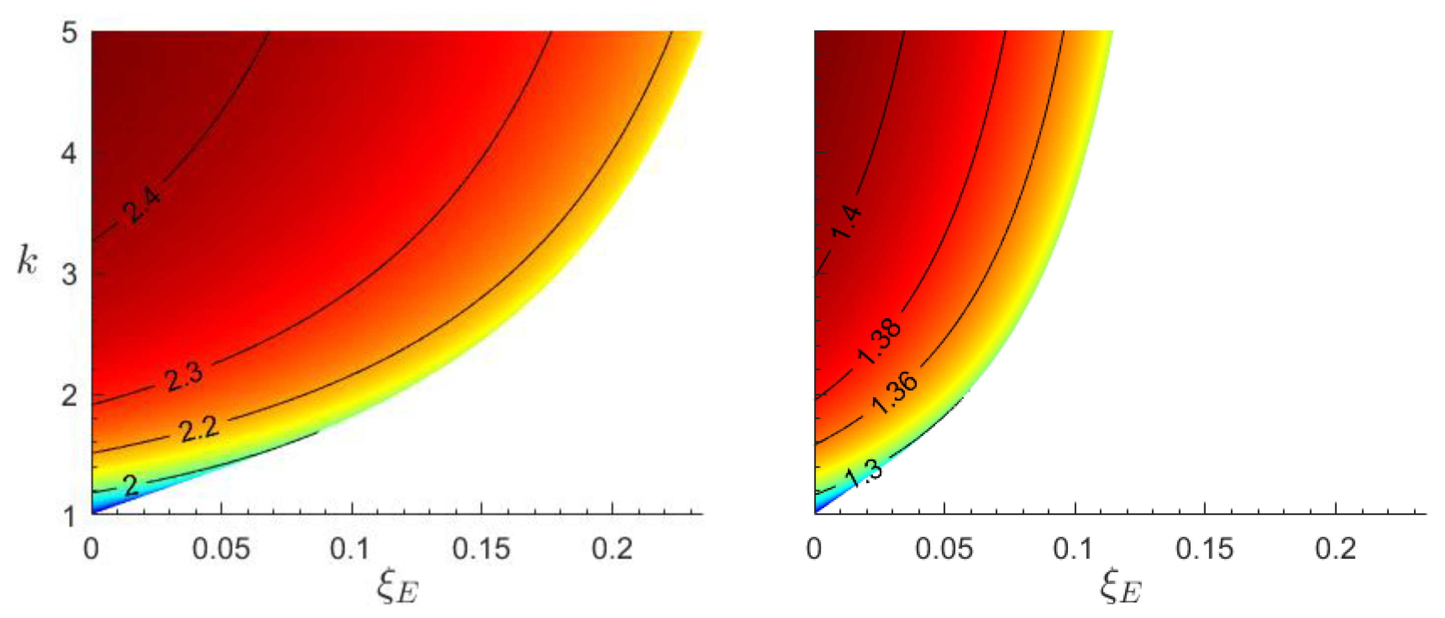
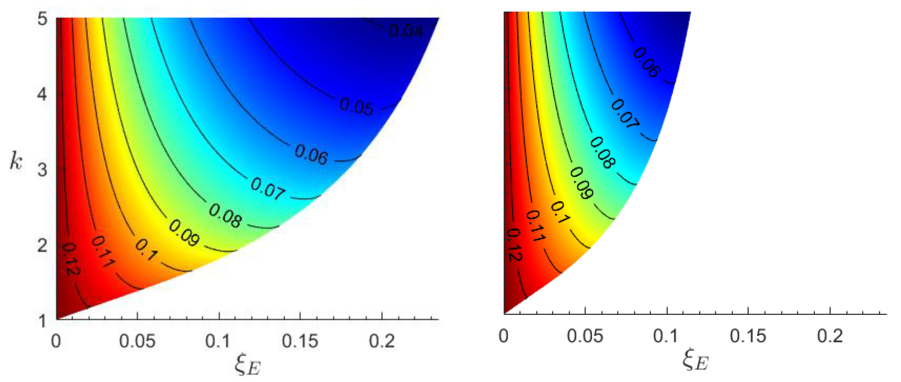
In a similar sense, the power characteristics at anti-resonance (Figure 10) also favor the PEH over the EMEH as the power rapidly declines at increasing ξ E and k , while it is close to its theoretical maximum for ξ E 1 , regardless of k .
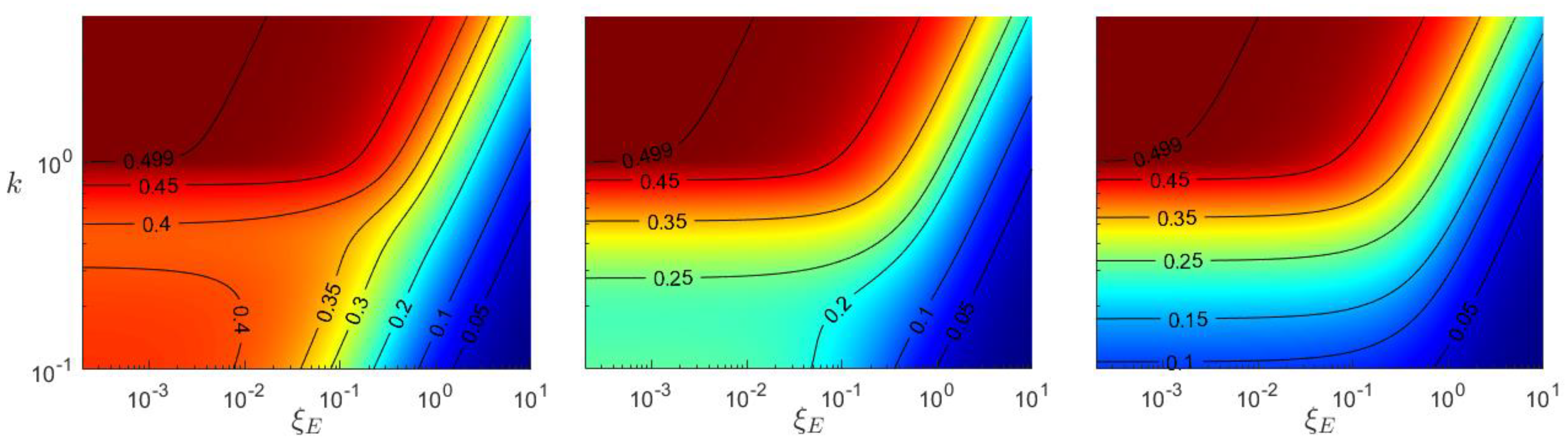
Assuming load and excitation frequency remain optimized by load power, both VEH systems have a maximum efficiency of 50% at resonance (see Figure 12). At anti-resonance, the efficiency is above 50% (if ξ E > 0 ) and increases along the boundary of k c r i t , in the direction of larger k and ξ E (see Figure 13). It may be beneficial to operate in this region if the source power is small, as the load power cannot be larger than efficiency times source power. If we instead assume an arbitrary γ and a load optimized by efficiency, a system with a larger η will have a larger maximum efficiency, although for γ 1 , the difference will be very small.

4.2. Comparison of Systems under Prescribed Displacement and Inertial Load

For the case of prescribed displacement and optimal load, the two systems (PEH/EMEH) have equivalent load power, which differs only in the relation to intrinsic electrical impedance. As the intrinsic impedance in an EMEH is in series with the load resistance, it should be minimized to maximize load power, and vice versa for the PEH.
Under the assumption of γ = 1 , we can extract an optimal load resistance from Equation (22) as:
EMEH :               R L _ P D _ o p t = ω L 2 + R W 2 PEH :                   R L _ P D _ o p t = 1 ω C P 2 + 1 R P 2
which shows that power optimization is achieved by impedance matching in this case. We compare this to the corresponding case of inertial load (see Equation (17)), which gives:
EMEH :                 R L _ I L _ o p t = ω L 2 + θ 2 C M + R W 2 PEH :                   R L _ I L _ o p t = 1 ω C P 2 + θ 2 C M + 1 R P 2
The above expression for optimal load resistance for an EMEH, under inertial load, can also be found in [6,14], under the assumption of negligible effect from inductance ( β 0 ) . The term θ 2 / C M in the optimal load for an EMEH, is in [14] defined as the electrical analogue of the mechanical damping. The same term appears in the optimal load expression for a PEH. In this case, the electrical analogue is equivalent to a resistance in parallel with the impedance, and thus becomes C M / θ 2 for a PEH. Although the electrical analogues are inverted between the systems, the series vs. parallel nature means the ratio θ 2 / C M should in both cases be minimized to achieve the highest possible power. This must be weighed against the negative effects of reducing the coupling factor, θ , or increasing the mechanical damping.
Intuitively, the difference in optimal load between the case of prescribed displacement and inertial load lies only in the electrical analogue to mechanical damping, which is only present in the case of inertial load. The comparison between the cases of inertial load and prescribed displacement thus supports the argument made by [14] that simple impedance matching does not provide the optimal load in the case of an energy harvester under inertial load.
Our results also show that applying the same resonant frequencies for the case of inertial load to the case of prescribed displacement generally leads to significantly larger dimensionless power output. This indicates that it may be beneficial to create a forced vibration of the proof mass if possible (e.g., by fixating to a surface that is static relative the vibrating surface). For the corresponding anti-resonant frequencies, this only holds for sufficiently small values of k and ξ E .

4.3. Comparison of PEH/EMEH Assuming Typical Parameter Values

Systems in the regime, Q Q c r i t ,   ξ E 1 and η 1 , are uncommon according to the small survey performed in [8]. This survey shows the typical case for an EMEH to be Q Q c r i t and ξ E 1 , and for a PEH it is Q < Q c r i t and ξ E 1 . Even though Q Q c r i t for an EMEH, it is still likely less than k c r i t Q c r i t , as k c r i t increases exponentially with ξ E (see Figure 3). This leads to both systems typically having only one power optimum, γ o p t _ R , corresponding to the resonant state. The same source, [8], states that η is typically small for a PEH (also mentioned in [1]) compared to an EMEH. Assuming η 1 (which implies Q c r i t 1 ) for the PEH, we can conclude that the typical case is that both systems have γ o p t _ R 1 .
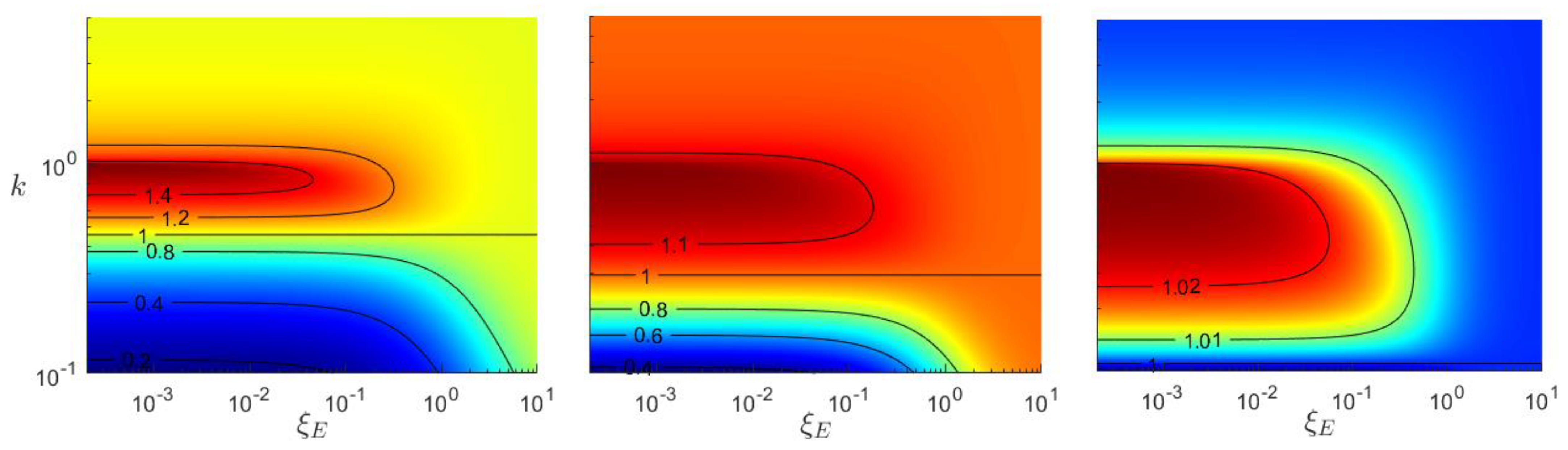
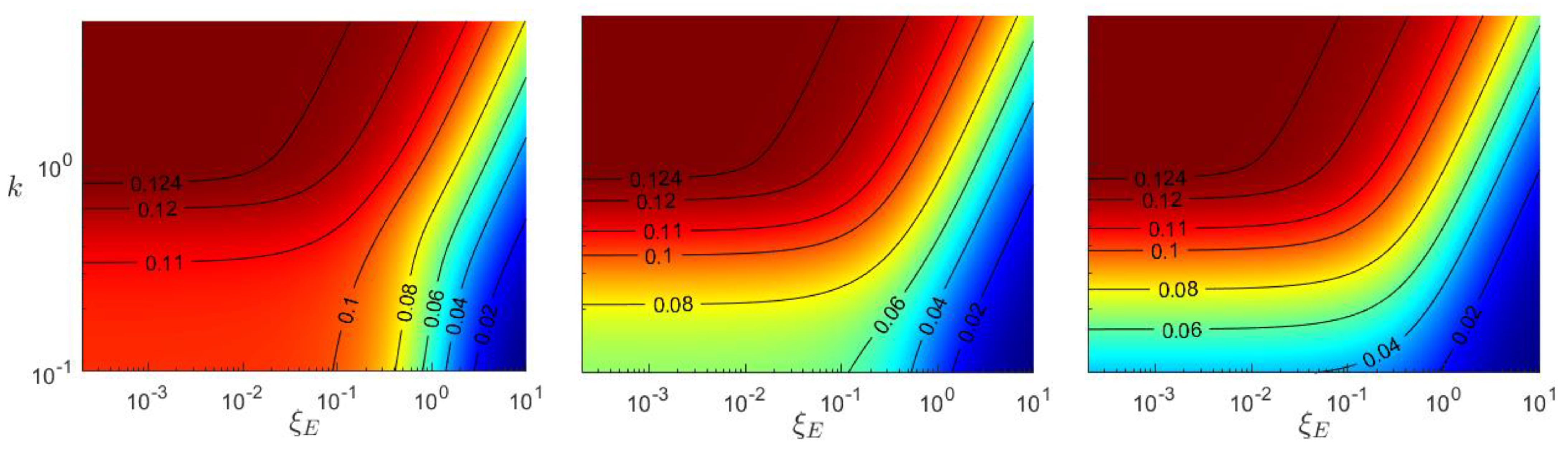
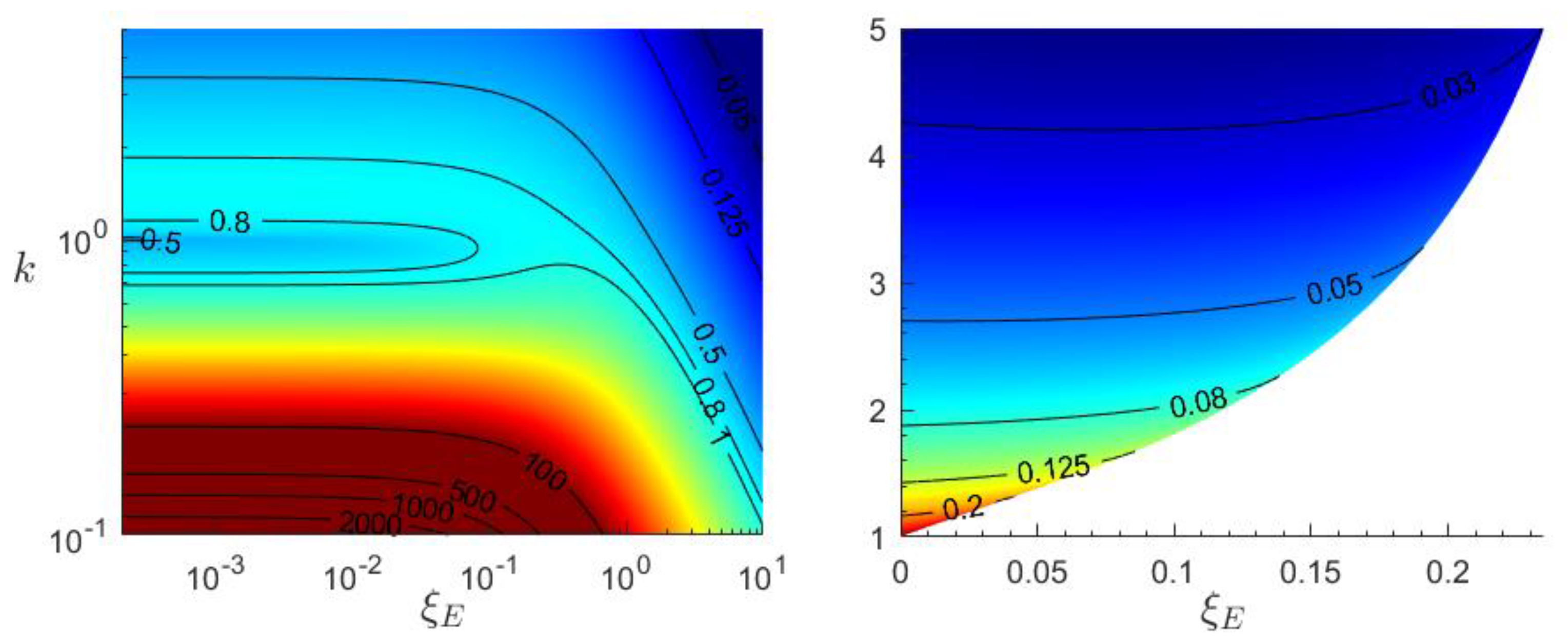
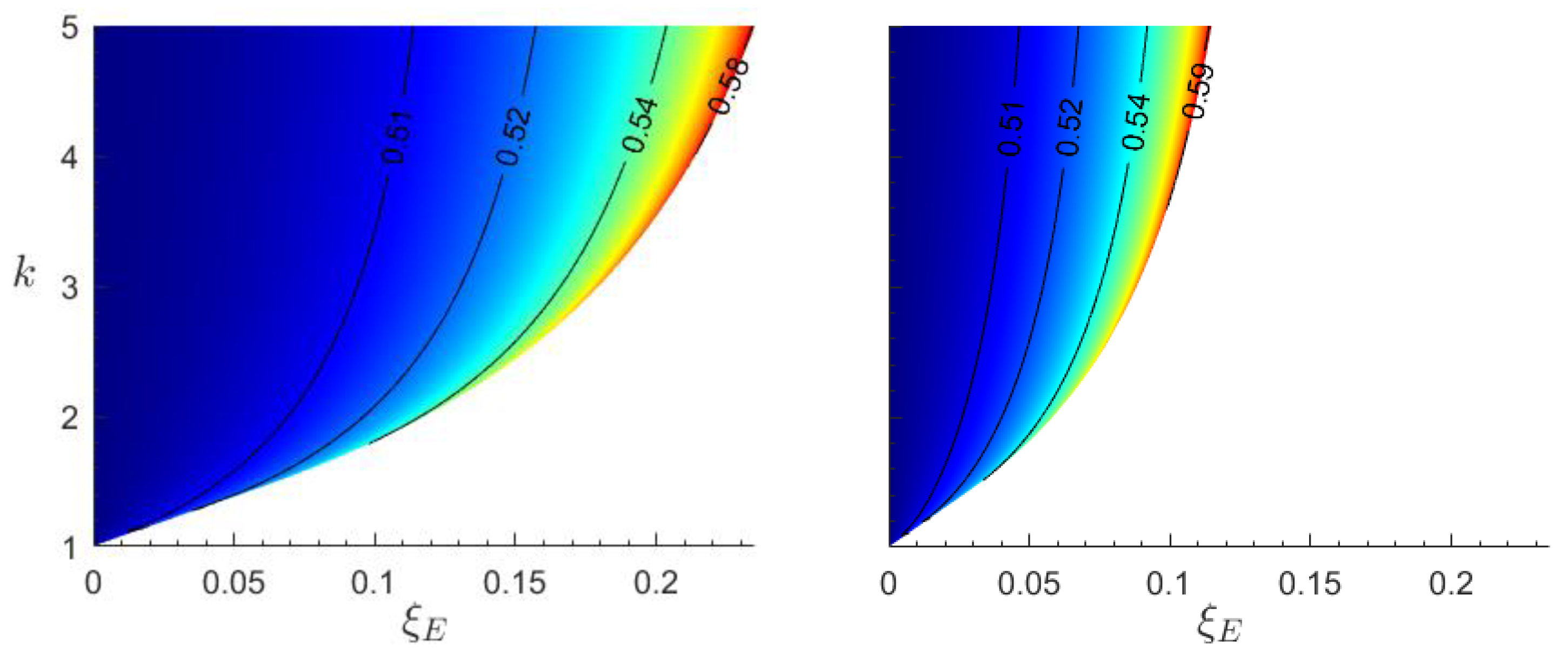
Using the typical values for Q and ξ E for an EMEH and PEH, respectively, we can state that power generated from an EMEH can be found in the upper right region of Figure 7 (left), while for the PEH it is found in the lower left region of Figure 7 (right). These numerical results indicate that, for a specific value of P ¯ , the dependance between k and ξ E has a constant linear slope in the logarithmic space, if k > 1 , with varying offset depending on the value of P ¯ . We find that, regardless of η , the linear slope in this region is approximately 1. The dependance between the ratio k / ξ E and value of P ¯ to be traced thus follows a logarithmic slope.
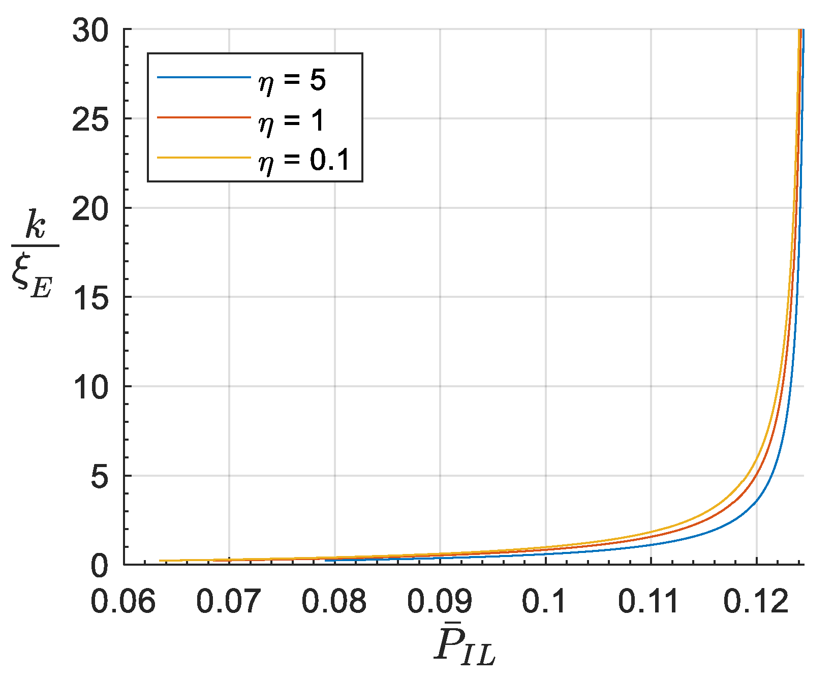
 Figure 15 shows k / ξ E as a function of P ¯ at η = 5 , 1 , 0.1 . We can see that the sensitivity of k to ξ E increases dramatically near the theoretical power maximum. The quality factor and/or effective coupling coefficient required to achieve a power output close to the theoretical maximum can thus become large for energy harvesters with a large loss coefficient, such as for a typical EMEH.
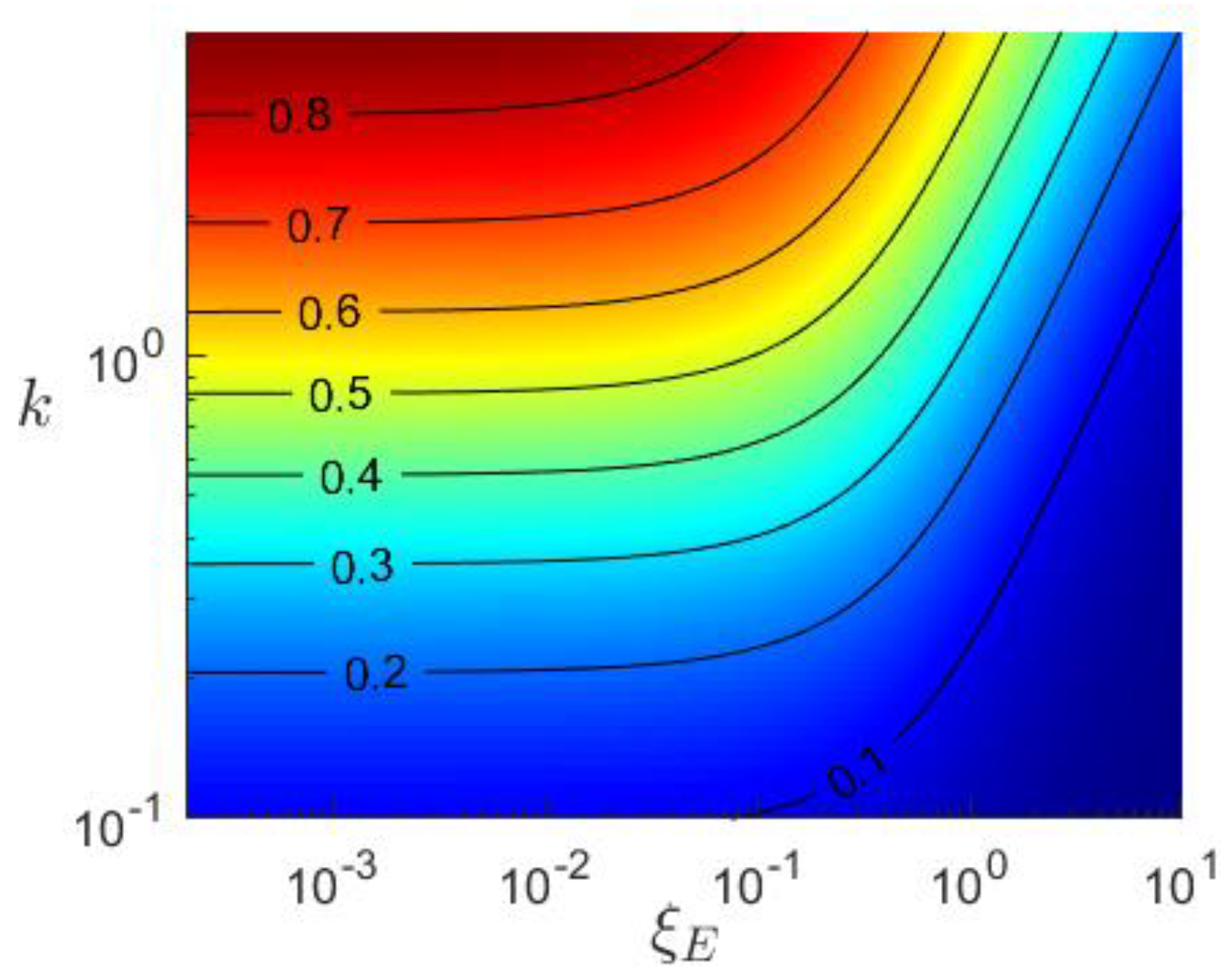
In the region of k < 1 and ξ E 1 , the sensitivity of k to ξ E is small. The power is in this region mainly a function of k and η . The goal for both types of energy harvesters should be to achieve a load power as close to the theoretical maximum as possible, without requiring a large quality factor, as the latter is equivalent to a small bandwidth. In both cases, η should be as large as possible, while k should be close to its critical value (see Figure 3). The loss factor, ξ E , typically only relevant for an EMEH, should be minimized.
The same arguments regarding load power can be applied to efficiency if load and excitation frequency remain optimized by load power.

4.4. Model Accuracy

Deriving an expression for the energy harvester power output, based on the lumped parameter model of Equation (1), and electric models of Equation (4), has been performed frequently in the previous literature. We compared our derived expression to those in [1,7,8,14] and found that, although different approaches are implemented and certain assumptions made, the resulting power expressions are equivalent. Measurements by duToit et al. [2] showed that the model significantly underpredicted measured PEH power output close to resonance and anti-resonance but was in good agreement off-resonance. Applying the model to the MEMS-scale EMEH in [4] results in a similar underprediction of the power at resonance. However, by reducing the input acceleration, an accurate prediction can be made even at resonance. This result is reasonable as the model is linear and will naturally break down outside of the linear regime. Arroyo et al. finds a good match between predicted and measured EMEH data at resonance while using a beam similar to that used by duToit et al., yet under a significantly larger base acceleration.
duToit et al. deduced the reason for their discrepancy to be the small-signal linear piezoelectric constitutive model, which underpredicted the piezoelectric constant at large strain. Triplett et al. [19] later confirmed that this nonlinear behavior is significant unless the tip displacement is small. Similarly, for the assumed case of a magnet traveling along the symmetry axis of a cylindrical coil, there are nonlinear effects in the electromechanical coupling of the EMEH arising from the nonlinear expansion of the magnetic field (along the symmetry axis) [4,5]. Thus, the requirement of small displacement is valid for an EMEH as well. Likewise, if we measure the coupling coefficient at a specific displacement amplitude and keep this parameter constant during measurements and calculations, the discrepancy between model and measurement due to nonlinear electromechanical coupling should be reduced.
For the model under inertial load, a constant base acceleration amplitude is assumed. This has a significant effect on the model output characteristics. As base acceleration amplitude equals ω 2 y 0 , where ω is angular excitation frequency and y 0 is the base displacement amplitude, this implies that either ω and y 0 are constant, and γ varies only due to spring stiffness and mass, or that y 0 is inversely proportional to ω . The latter case breaks down as γ approaches zero as this implies y 0 . The alternative is that ω remains constant and the ratio of spring stiffness to mass approaches infinity, which is a feasible case.

5. Conclusions

This article sets out to provide an increased understanding of piezo- and magnetoelectric energy harvesting systems and their combination, and to develop a tool to aid the development of harvester prototypes.
We achieve this objective by deriving general expressions for PEH/EMEH power output, using the full set of relevant dimensionless parameters, γ , Q , ξ E , ξ C and η . While the model does not account in a direct way for nonlinear effects, it conveys an understanding of the behavior throughout the parameter space. Once the region of interest has been identified, one can apply refined nonlinear models. In this sense, the model helps in the choice of a suitable transduction method for a specific application as well as for the design of energy harvesters.
To shed new light on previously well-established VEH systems, we perform a detailed analysis with regard to the resistive loss coefficient, which is lacking in the previous literature. We find that this parameter plays a significant role in differentiating inertially loaded PEH/EMEH systems, especially in the context of resonant and anti-resonant operation. We find that at resonance, both systems have similar potential power performance, with the EMEH being favored due to a potentially larger load voltage. At anti-resonance, the PEH is favored both in regard to power output and voltage. Our results show a larger input to output power efficiency at anti-resonance compared to resonance. It can thus be beneficial to run the VEH with a larger load resistance in cases where the source power is small, assuming the source vibration spectrum is similar around the energy harvester’s resonance and anti-resonance frequencies.
Considering typical parameter values for applied EMEH/PEH systems, we can conclude that they are generally designed to operate at resonance. Under these assumptions, we can still draw some important conclusions. Compared with a PEH, an EMEH will be practically limited in achieving a power output closer to the theoretical maximum, less sensitive to resistive loss with regard to critical Q factor and have an optimal load highly sensitive to the quality factor.
Our investigation of the model under prescribed displacement, which is also lacking in the previous literature, shows that the expression for efficiency is equal to that of the model under inertial load, which is a reasonable result assuming efficiency is a purely intrinsic property (independent of external excitation). We also find that the expressions for optimal load differ between the two types of excitations only by the term naturally arising from electrical damping, supporting the argument that impedance matching is not the correct approach to load optimization of inertially loaded systems. From a practical viewpoint, our results indicate that under resonant excitation frequencies, a higher dimensionless power can generally be achieved if the proof mass oscillations can be forced. At anti-resonant frequencies, this is only holds for sufficiently small k and ξ E .
Thanks to the detailed investigation of the resistive loss coefficient and the case of prescribed displacement, our investigation essentially widens the range of potential methods that may be used to find high-performance VEH designs and thus increases the possibility of VEHs being useful in an increasing number of applications.

Supplementary Materials

The following supporting information can be downloaded at: https://www.mdpi.com/article/10.3390/app12199815/s1.

Author Contributions

Conceptualization, J.B., F.O., C.R. and C.J.; Formal analysis, J.B.; Funding acquisition, C.R.; Investigation, J.B.; Methodology, J.B., F.O. and C.J.; Project administration, C.R.; Resources, C.R.; Software, J.B.; Supervision, C.R.; Validation, J.B., F.O. and C.J.; Visualization, J.B.; Writing—original draft, J.B.; Writing—review and editing, J.B., F.O., C.R. and C.J. All authors have read and agreed to the published version of the manuscript.

Funding

This work received funding from Swedish Foundation for Strategic Research in the program for ‘Research Institute PhD’ (grant no. FID16-0055) and from ECSEL Joint Undertaking (JU) project ‘Energy ECS’ (grant no. 101007247). The APC was funded by RISE Research Institutes of Sweden AB.

Institutional Review Board Statement

Not applicable.

Informed Consent Statement

Not applicable.

Data Availability Statement

Not applicable.

Conflicts of Interest

The authors declare no conflict of interest.

References

  1. Yang, Z.; Erturk, A.; Zu, J. On the efficiency of piezoelectric energy harvesters. Extrem. Mech. Lett. 2017, 15, 26–37. [Google Scholar] [CrossRef]
  2. duToit, N.E.; Wardle, B.L. Experimental Verification of Models for Microfabricated Piezoelectric Vibration Energy Harvesters. AIAA J. 2007, 4, 1126–1137. [Google Scholar] [CrossRef]
  3. Liao, Y.; Sodano, H. Optimal power, power limit and damping of vibration based piezoelectric power harvesters. Smart Mater. Struct. 2018, 27, 75057. [Google Scholar] [CrossRef]
  4. Beeby, S.P.; Torah, R.N.; Tudor, M.J.; Glynne-Jones, P.; O’Donnell, T.; Saha, C.R.; Roy, S. A micro electromagnetic generator for vibration energy harvesting. J. Micromech. Microeng. 2007, 17, 1257–1265. [Google Scholar] [CrossRef]
  5. Kecik, K.; Kowalczuk, M. Effect of Nonlinear Electromechanical Coupling in Magnetic Levitation Energy Harvester. Energies 2021, 14, 2715. [Google Scholar] [CrossRef]
  6. Phan, T.N.; Aranda, J.J.; Oelmann, B.; Bader, S. Design Optimization and Comparison of Cylindrical Electromagnetic Vibration Energy Harvesters. Sensors 2021, 21, 7985. [Google Scholar] [CrossRef] [PubMed]
  7. Wang, X.; John, S.; Watkins, S.; Yu, X.; Xiao, H.; Liang, X.; Wei, H. Similarity and duality of electromagnetic and piezoelectric vibration energy harvesters. Mech. Syst. Signal. Process. 2015, 52–53, 672–684. [Google Scholar] [CrossRef]
  8. Arroyo, E.; Badel, A.; Formosa, F.; Wu, Y.; Qiu, J. Comparison of electromagnetic and piezoelectric vibration energy harvesters: Model and experiments. Sens. Actuators A Phys. 2012, 183, 148–156. [Google Scholar] [CrossRef]
  9. Poulin, G.; Sarraute, E.; Costa, F. Generation of electrical energy for portable devices. Sens. Actuators A Phys. 2004, 116, 461–471. [Google Scholar] [CrossRef]
  10. Wang, X.; Liang, X.; Wei, H. A study of electromagnetic vibration energy harvesters with different interface circuits. Mech. Syst. Signal. Process. 2015, 58–59, 376–398. [Google Scholar] [CrossRef]
  11. Wang, X.; Lin, L. Dimensionless optimization of piezoelectric vibration energy harvesters with different interface circuits. Smart Mater. Struct. 2013, 22, 85011. [Google Scholar] [CrossRef]
  12. Wang, X. A study of harvested power and energy harvesting efficiency using frequency response analyses of power variables. Mech. Syst. Signal. Process. 2019, 133, 106277. [Google Scholar] [CrossRef]
  13. Wang, X. Coupling loss factor of linear vibration energy harvesting systems in a framework of statistical energy analysis. J. Sound Vib. 2016, 362, 125–141. [Google Scholar] [CrossRef]
  14. Stephen, N.G. On energy harvesting from ambient vibration. J. Sound Vib. 2006, 293, 409–425. [Google Scholar] [CrossRef]
  15. Tai, W.-C.; Zuo, L. On optimization of energy harvesting from base-excited vibration. J. Sound Vib. 2017, 411, 47–59. [Google Scholar] [CrossRef]
  16. Liao, Y.; Liang, J. Generalized modeling and analysis of piezoelectric vibration energy harvesters. In Active and Passive Smart Structures and Integrated Systems XIII; Erturk, A., Ed.; SPIE: Bellingham, WA, USA, 2019; p. 75. [Google Scholar] [CrossRef]
  17. Kim, M.; Dugundji, J.; Wardle, B.L. Efficiency of piezoelectric mechanical vibration energy harvesting. Smart Mater. Struct. 2015, 24, 55006. [Google Scholar] [CrossRef]
  18. Kunz, J.; Fialka, J.; Pikula, S.; Benes, P.; Krejci, J.; Klusacek, S.; Havranek, Z. A New Method to Perform Direct Efficiency Measurement and Power Flow Analysis in Vibration Energy Harvesters. Sensors 2021, 21, 2388. [Google Scholar] [CrossRef] [PubMed]
  19. Triplett, A.; Quinn, D.D. The Effect of Non-linear Piezoelectric Coupling on Vibration-based Energy Harvesting. J. Intell. Mater. Syst. Struct. 2009, 20, 1959–1967. [Google Scholar] [CrossRef]
Figure 1. Representation of PEH (left) and EMEH (middle), with a corresponding free-body diagram (right). C E and C M are the electrical and mechanical damping coefficients. K M is the mechanical spring coefficient. m is the effective mass of the system. x t is the proof mass or tip displacement, and y t is the base displacement.
Applsci 12 09815 g001
Figure 2. Lumped element model of electrical domain. Left: EMEH. L , R w and R L are the coil inductance, coil resistance and load resistance. v is the generated voltage, and i is the resulting current. Right: PEH. C P , R P and R L are the capacitance, resistance due to PEH resistivity and load resistance. i is the generated current, and v is the resulting voltage.
Applsci 12 09815 g002
Figure 3. Minimum value of k required for the existence of an anti-resonant solution. η = 0.1 ,   0.5 ,   1 ,   5 , from left to right.
Applsci 12 09815 g003
Figure 4. Normalized angular excitation frequency at resonance, under the condition of power optimal load. η = 5 ,   1 ,   0.1 , from left to right. The color scale is linear and independent for each plot. Y axis is identical for each plot but only specified in the left plot.
Applsci 12 09815 g004
Figure 5. Power-optimum normalized load resistance, at resonant excitation frequency. η = 5 ,   1 ,   0.1 , from left to right. The color scale is logarithmic and independent for each plot. Y axis is identical for each plot but only specified in the left plot.
Applsci 12 09815 g005
Figure 6. Power-optimum normalized load resistance, at resonant excitation frequency. η = 5 ,   0.1 and ξ E = 0 ,   0.1 .
Applsci 12 09815 g006
Figure 7. Dimensionless power at optimal load and resonant excitation frequency. η = 5 ,   1 ,   0.1 , from left to right. The color scale is linear and independent for each plot. Y axis is identical for each plot but only specified in the left plot.
Applsci 12 09815 g007
Figure 8. Normalized angular excitation frequency at anti-resonance and power optimal load. η = 5 ,   1 , from left to right. The color scale is linear and independent for each plot. Y axis is identical for both plots but only specified in the left plot.
Applsci 12 09815 g008
Figure 9. Power-optimum normalized load resistance at anti-resonant excitation frequency. η = 5 ,   1 , from left to right. The color scale is logarithmic and independent for each plot. Y axis is identical for both plots but only specified in the left plot.
Applsci 12 09815 g009
Figure 10. Dimensionless power at optimal load and anti-resonant excitation frequency. η = 5 ,   1 , from left to right. The color scale is linear and independent for each plot. Y axis is identical for both plots but only specified in the left plot.
Applsci 12 09815 g010
Figure 11. Dimensionless power under prescribed displacement, assuming the excitation frequency is equal to the power optimal case with inertial load. The load here is optimized for the case of prescribed displacement, and η is set to 5. The same parameter definitions as in Table 1 and Table 2 are assumed when using Equation (23). Left: resonant frequencies. Right: anti-resonant frequencies. The color scale is logarithmic and independent for each plot. Y axis represents the parameter k in both plots.
Applsci 12 09815 g011
Figure 12. Power input to output efficiency under the condition of power optimal load and resonant excitation frequency. η = 5 ,   1 ,   0.1 , from left to right. The color scale is linear and independent for each plot. Y axis is identical for each plot but only specified in the left plot.
Applsci 12 09815 g012
Figure 13. Power input to output efficiency under the condition of power optimal load and anti-resonant excitation frequency. η = 5 ,   1 , from left to right. The color scale is linear and independent for each plot. Y axis is identical for both plots but only specified in the left plot.
Applsci 12 09815 g013
Figure 14. Power input to output efficiency under the condition of efficiency optimal load and resonant excitation frequency. γ = 1 and η = 1 . The color scale is linear.
Applsci 12 09815 g014
Figure 15. Sensitivity of k to ξ E as a function of dimensionless power, i.e., the ratio of k to ξ E when tracing a specific power value. This relationship only holds for k > 1.
Applsci 12 09815 g015
Table 1. Dimensionless parameters.
ParameterExpressionName
Q m ω N / C M Mechanical quality factor ω N = K M / m
ζ 1 / 2 Q Mechanical damping ratio
η θ 2 / K M B Effective electromechanical coupling coefficient
γ ω / ω N Normalized angular excitation frequency
ξ C P E H :   1 / R L ω N B
E M E H :   R L / ω N B
Load coefficient
ξ E P E H :   1 / R P ω N B
E M E H :   R W / ω N B
Resistive loss coefficient
Table 2. Dimensionless parameters used to simplify the power expression.
ParameterExpression
α θ 2 / C M A
β 1 / ( ξ C + ξ E )
ε Q γ 2 1 / γ
Publisher’s Note: MDPI stays neutral with regard to jurisdictional claims in published maps and institutional affiliations.

