

A Hybrid Golden Jackal Optimization and Golden Sine Algorithm with Dynamic Lens-Imaging Learning for Global Optimization Problems

Abstract
:1. Introduction
- (1)
- LSGJO is proposed.
- (2)
- Wilcoxon rank sum test and Friedman test are used to analyze the statistical data. Observing the convergence curve and comparing it with other algorithms proves that LSGJO has tremendous advantages.
- (3)
- LSGJO is applied to solve three constrained optimization problems in mechanical fields and compared with many advanced algorithms.
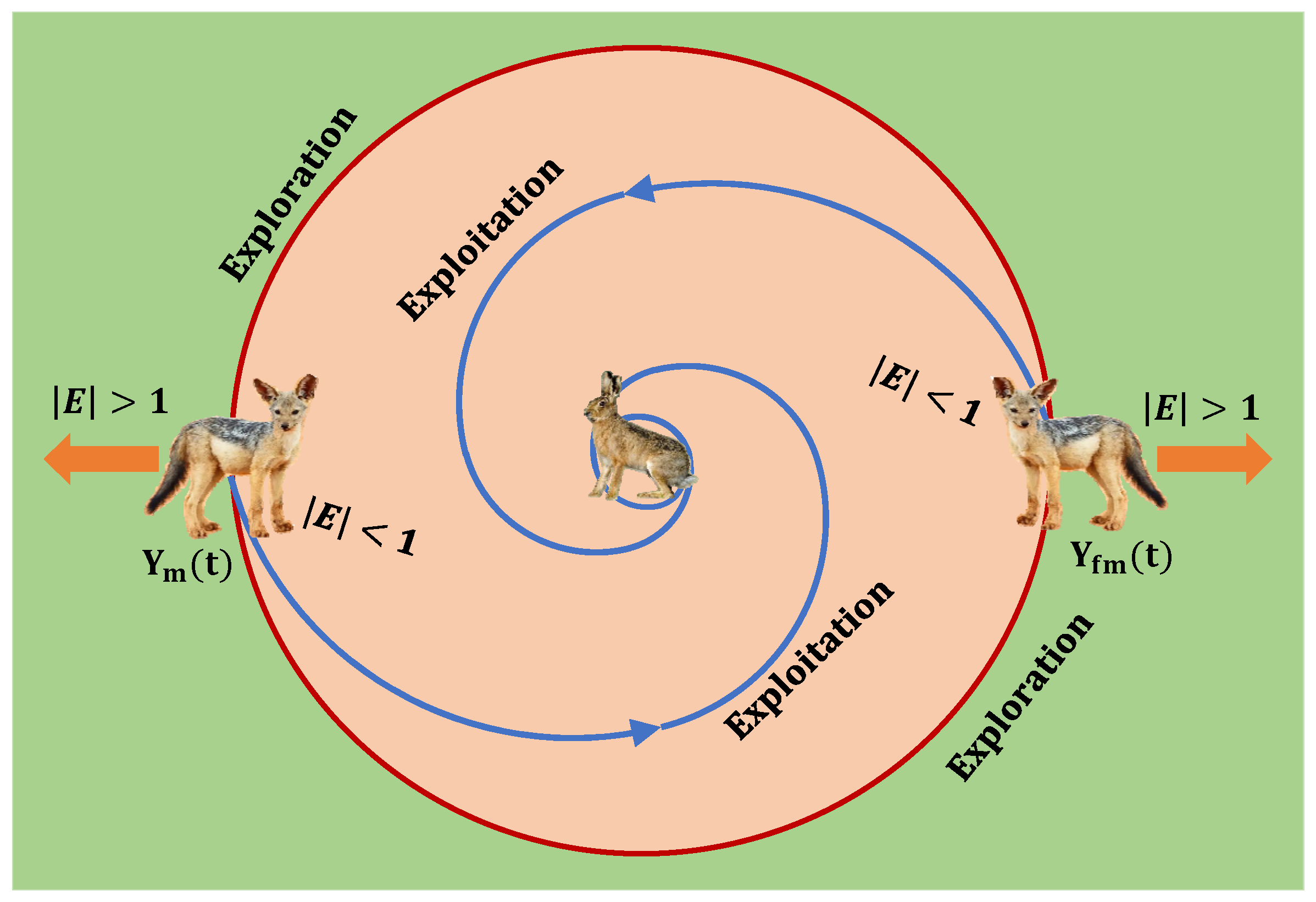
2. Golden Jackal Algorithm
| Algorithm 1: Golden Jackal Optimization |
| Inputs: The population size N and maximum number of iterations T Outputs: The location of prey and its fitness value Initialize the random prey population (i = 1, 2, …, N) While (t < T) Calculate the fitness values of prey = best prey individual (Male Jackal Position) = second best prey individual (Female Jackal Position) for (each prey individual) Update the evading energy “E” using Equations (4) and (6) Update “rl” using Equations (6) and (7) If (|E| ≤ 1) (Exploration phase) Update the prey position using Equations (2), (3), and (8) If (|E| > 1) (Exploitation phase) Update the prey position using Equations (8), (9), and (10) end for t = t + 1 end while return |
3. Proposed LSGJO
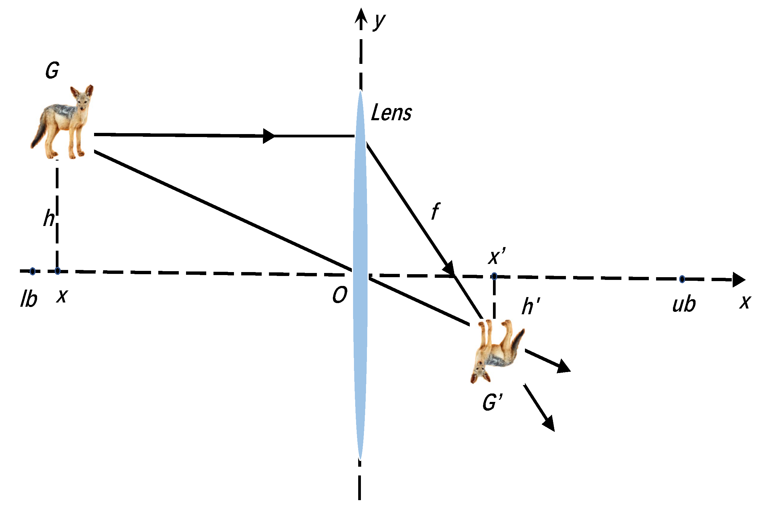
3.1. Dynamic Lens-Imaging Learning Strategy
3.2. Novel Update Rules
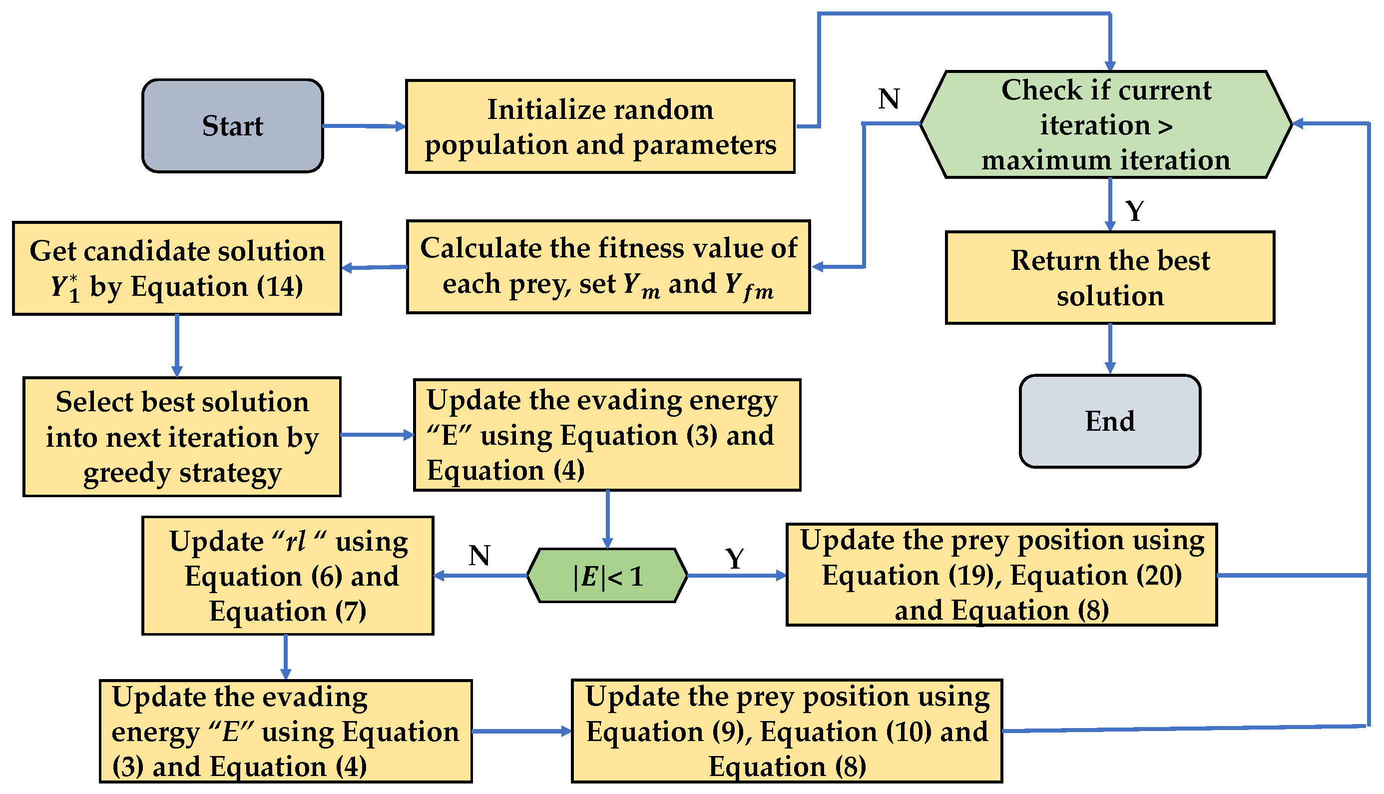
| Algorithm 2: The pseudo-code of LSGJO |
| Inputs: The population size N and maximum number of iterations T Outputs: The location of prey and its fitness value Initialize the random prey population (i = 1, 2, …, N) While (t < T) Calculate the fitness values of prey = best prey individual (Male Jackal Position) = second best prey individual (Female Jackal Position) Obtain by Equation (14) Calculate the fitness function values of and , set the better one as for (each prey individual) Update the evading energy “E” using Equations (3) and (4) Update “rl” using Equations (6) and (7) If(|E| ≥ 1) (Exploration phase) Update the prey position using Equations (8), (19), and (20) If(|E| < 1) (Exploitation phase) Update the prey position using Equations (8), (9), and (10) end for t = t + 1 end while return |
3.3. The Computational Complexity of LSGJO
4. Simulation and Result Analysis
4.1. Comparison and Analysis with Metaheuristic Algorithms
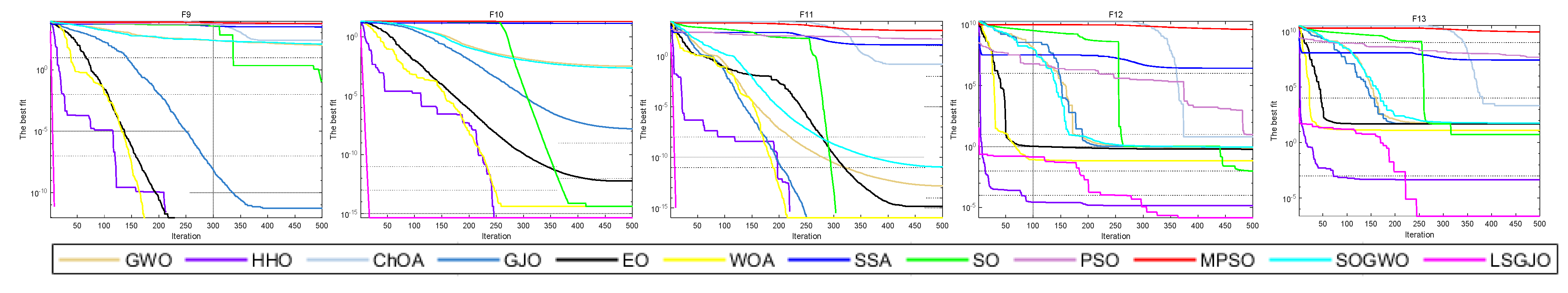
4.2. Experimental Analysis of the Algorithm in Different Dimensions of Function
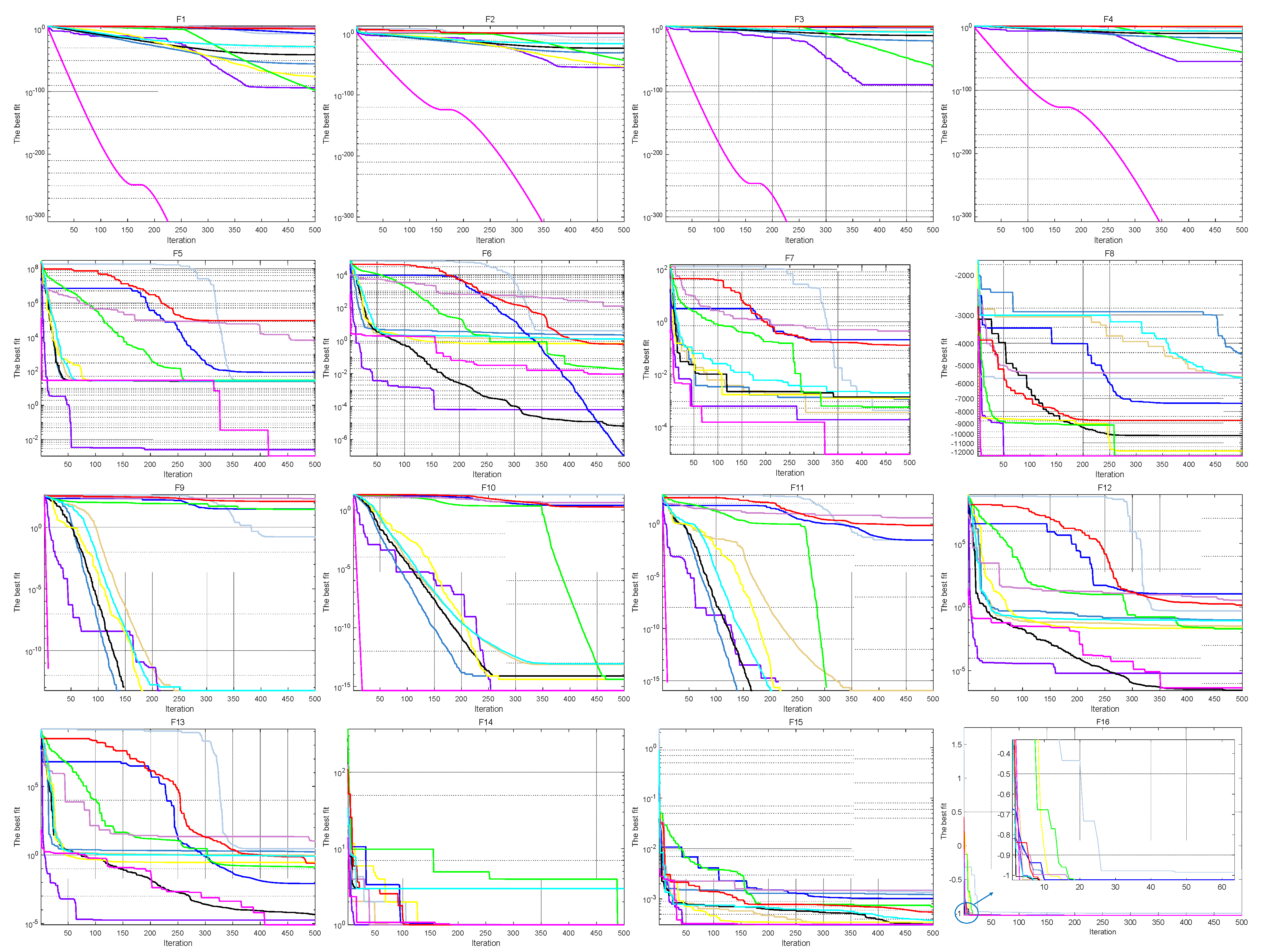
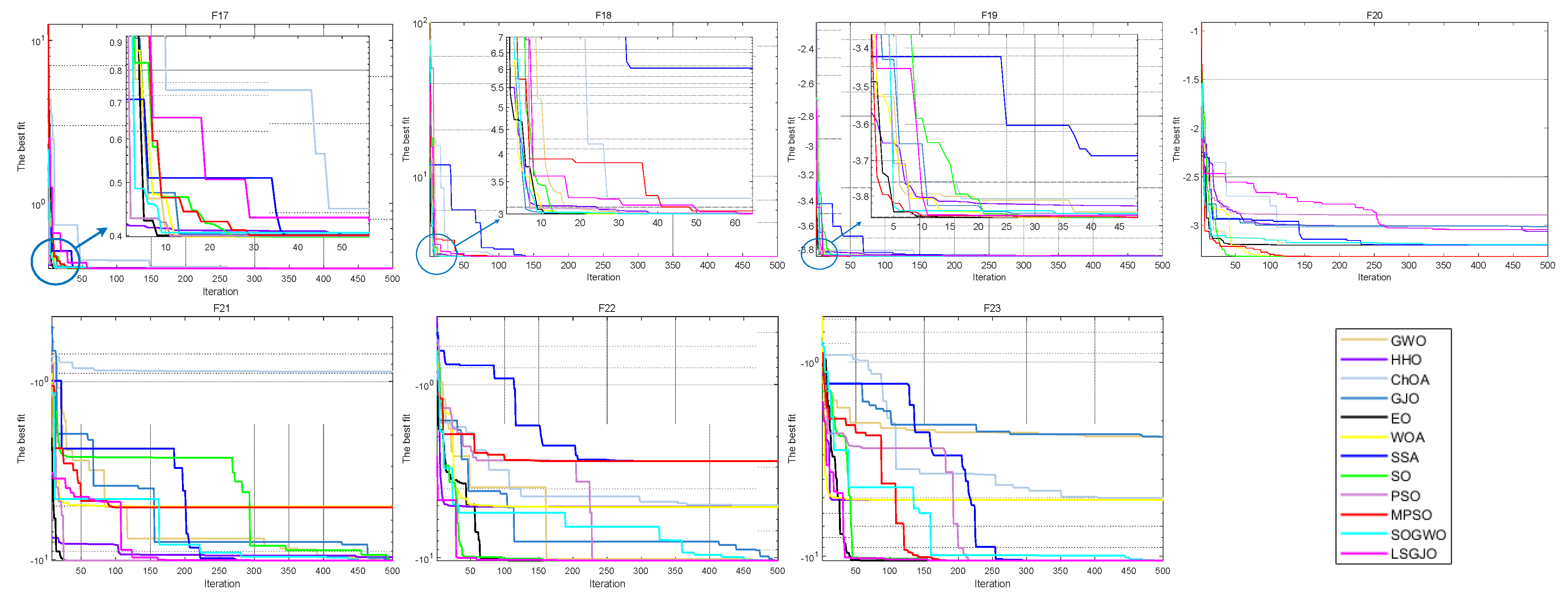
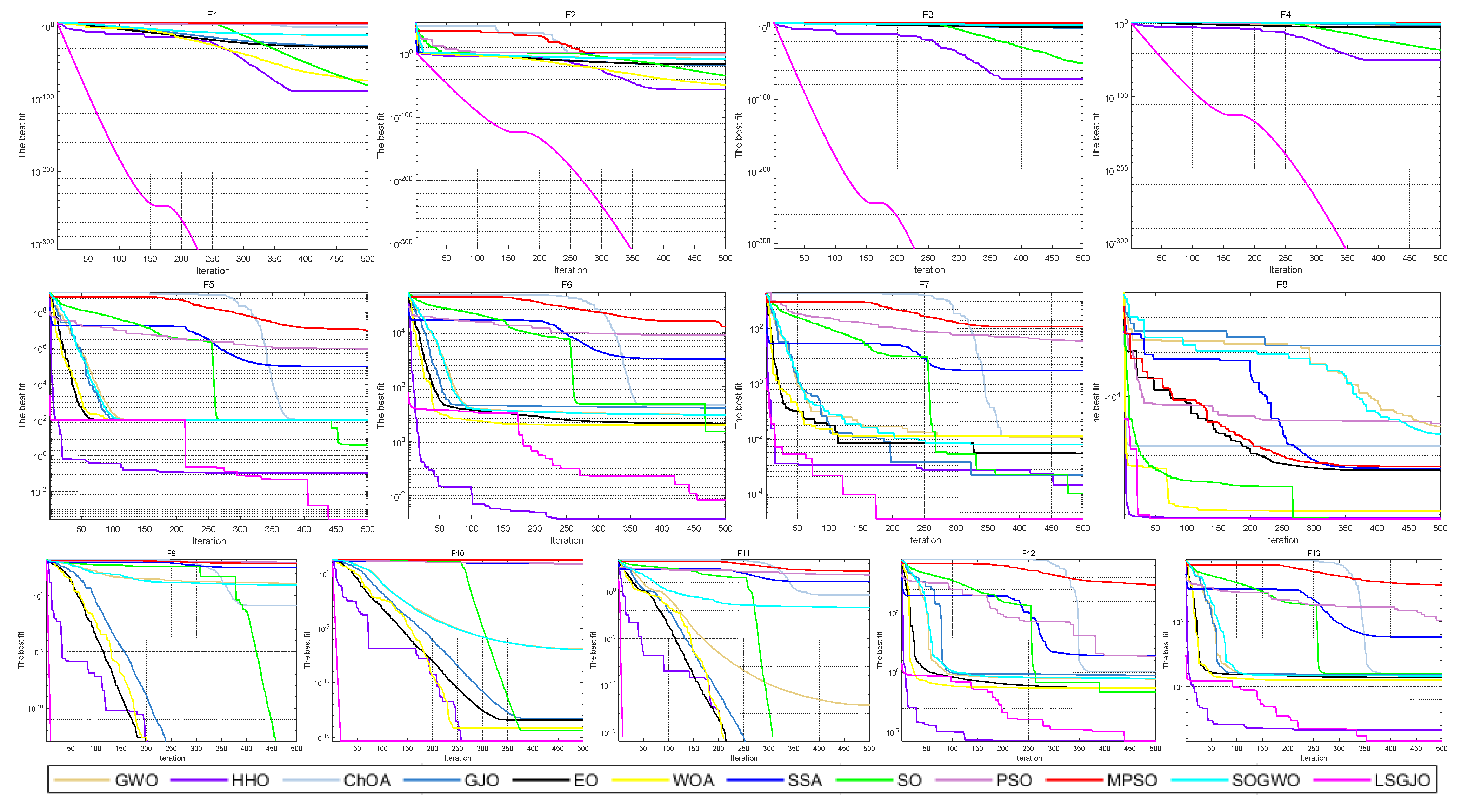
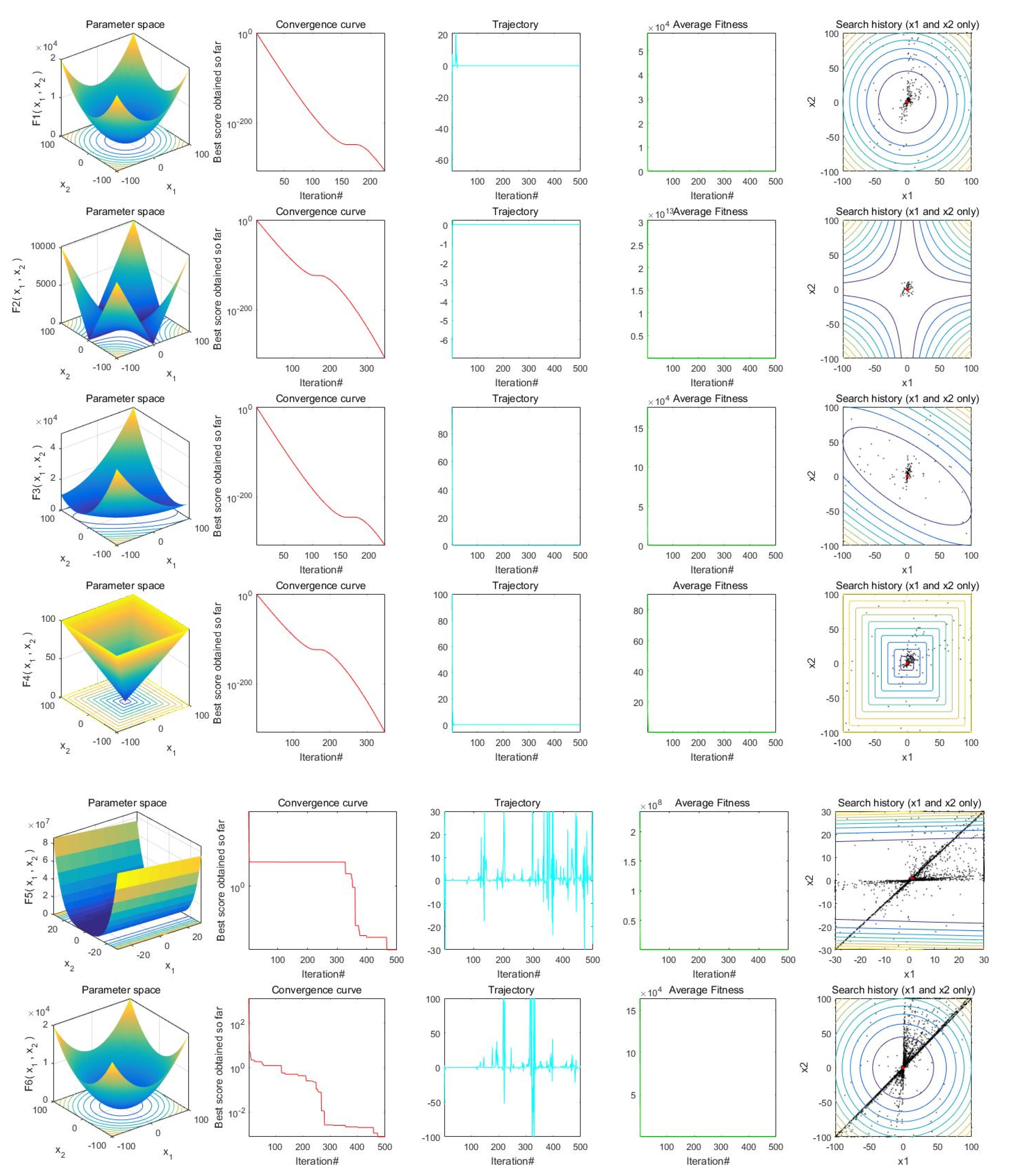
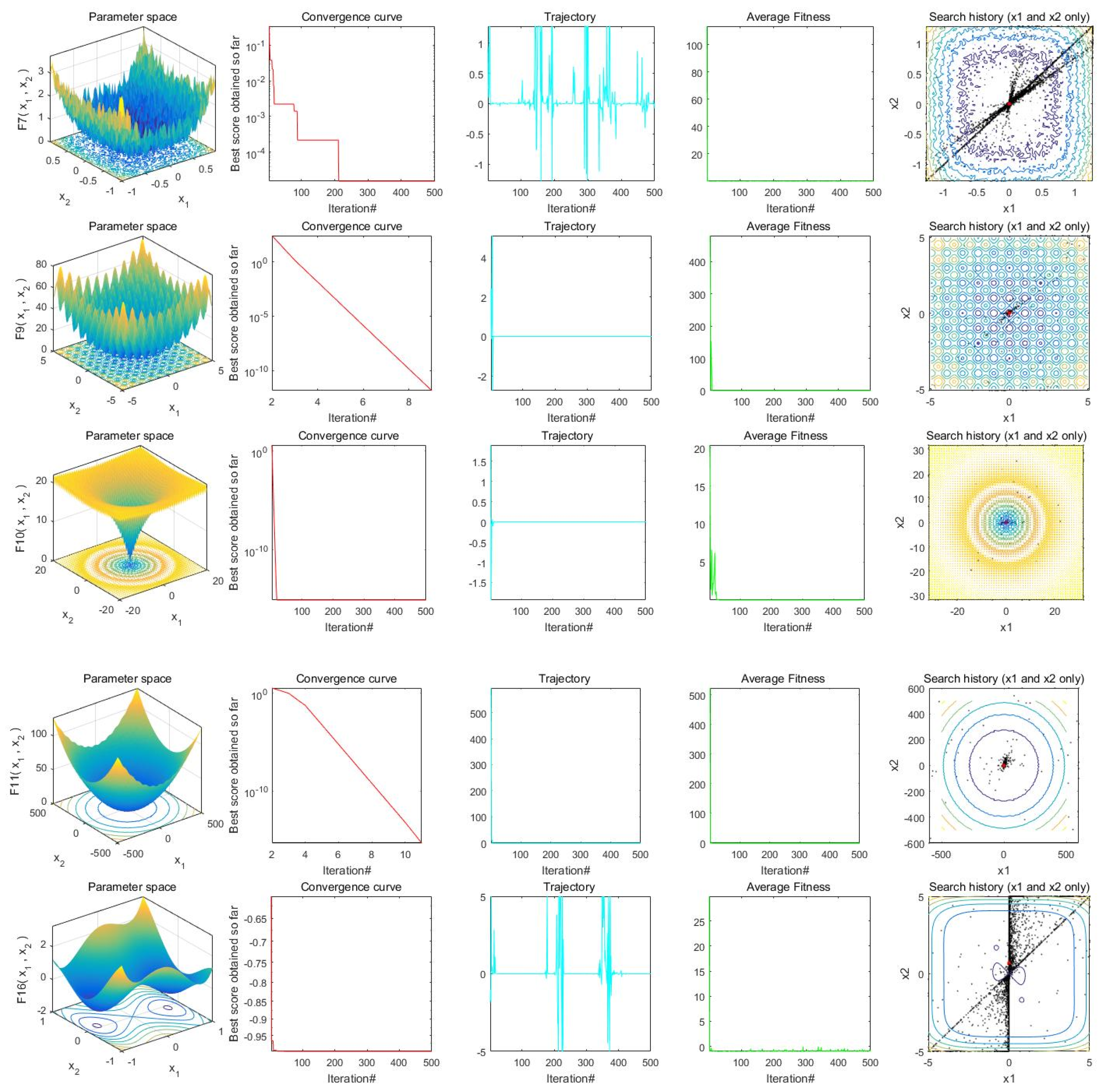
4.3. Convergence Behavior Analysis
4.4. Statistical Analysis
5. Real-World Engineering Design Problems
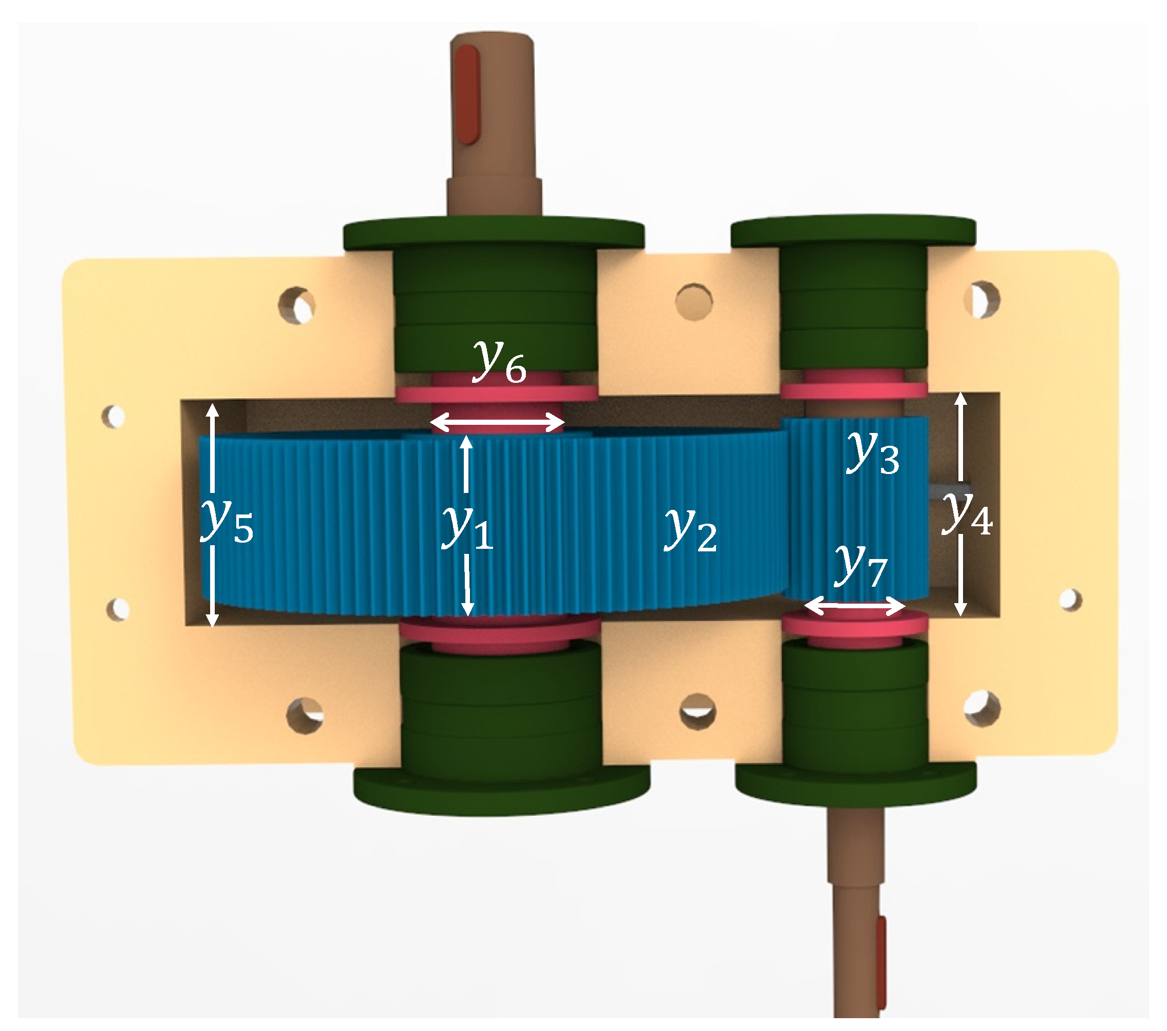
5.1. Speed Reducer Design Problem
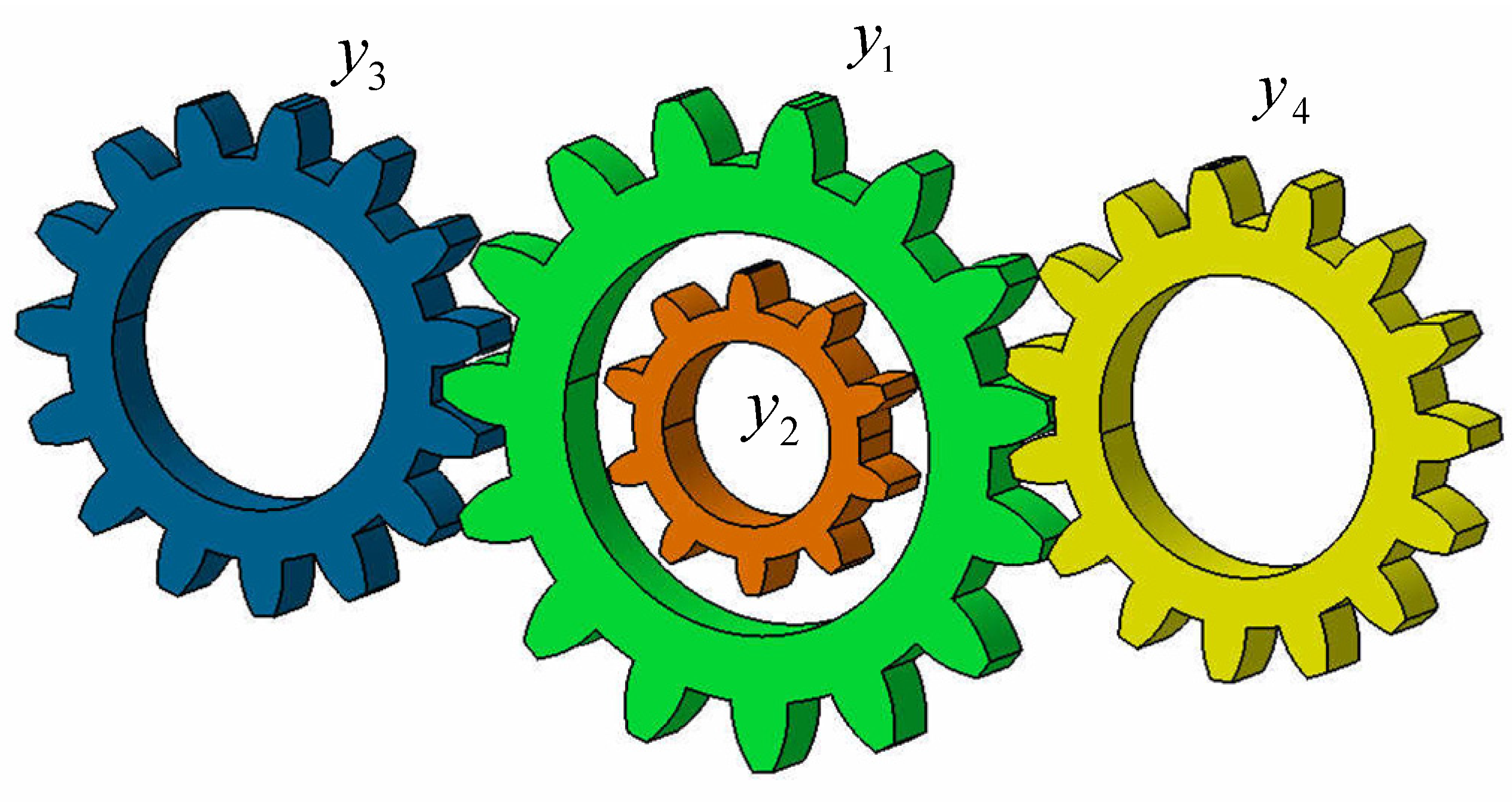
5.2. Gear Train Design Problem
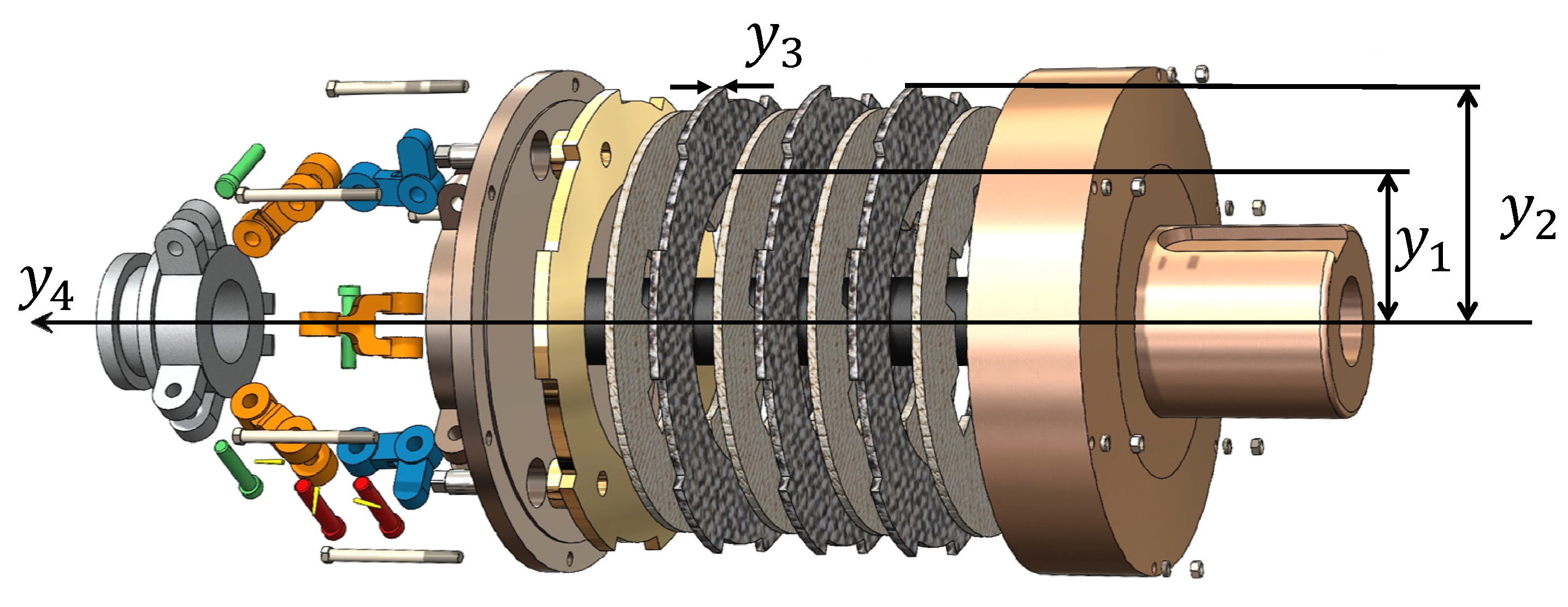
5.3. Multiple-Disk Clutch Design Problem
6. Discussion
7. Conclusions
Author Contributions
Funding
Institutional Review Board Statement
Informed Consent Statement
Data Availability Statement
Conflicts of Interest
Appendix A
References
- Wu, G. Across neighborhood search for numerical optimization. Inf. Sci. 2016, 329, 597–618. [Google Scholar] [CrossRef]
- Tanyildizi, E.; Demir, G. Golden Sine Algorithm: A Novel Math-Inspired Algorithm. Adv. Electr. Comput. Eng. 2017, 17, 71–78. [Google Scholar] [CrossRef]
- Sun, X.X.; Pan, J.S.; Chu, S.C.; Hu, P.; Tian, A.Q. A novel pigeon-inspired optimization with QUasi-Affine TRansfor-mationevolutionary algorithm for DV-Hop in wireless sensor networks. Int. J. Distrib. Sens. Netw. 2020, 16, 1–15. [Google Scholar] [CrossRef]
- Song, P.C.; Chu, S.C.; Pan, J.S.; Yang, H. Simplified Phasmatodea population evolution algorithm for optimization. Complex Intell. Syst. 2022, 8, 2749–2767. [Google Scholar] [CrossRef]
- Sun, L.; Koopialipoor, M.; Armaghani, D.J.; Tarinejad, R.; Tahir, M. Applying a meta-heuristic algorithm to predict and op-timize compressive strength of concrete samples. Eng. Comput. 2019, 37, 1133–1145. [Google Scholar] [CrossRef]
- Mirjalili, S.; Lewis, A. The whale optimization algorithm. Adv. Eng. Softw. 2016, 95, 51–67. [Google Scholar] [CrossRef]
- Mirjalili, S.; Gandomi, A.H.; Mirjalili, S.Z.; Saremi, S.; Faris, H.; Mirjalili, S.M. Salp Swarm Algorithm: A bio-inspired optimizer for engineering design problems. Adv. Eng. Softw. 2017, 114, 163–191. [Google Scholar] [CrossRef]
- Heidari, A.A.; Mirjalili, S.; Faris, H.; Aljarah, I.; Mafarja, M.; Chen, H. Harris hawks optimization: Algorithm and applications. Future Gener. Comput. Syst. 2019, 97, 849–872. [Google Scholar] [CrossRef]
- Faramarzi, A.; Heidarinejad, M.; Stephens, B.; Mirjalili, S. Equilibrium optimizer: A novel optimization algorithm. Knowl.-Based Syst. 2019, 191, 105190. [Google Scholar] [CrossRef]
- Nematollahi, A.F.; Rahiminejad, A.; Vahidi, B. A novel physical based meta-heuristic optimization method known as lightning attachment procedure optimization. Appl. Soft Comput. 2017, 59, 596–621. [Google Scholar] [CrossRef]
- Ghasemi, M.; Davoudkhani, I.F.; Akbari, E.; Rahimnejad, A.; Ghavidel, S.; Li, L. A novel and effective optimization algorithm for global optimization and its engineering applications: Turbulent Flow of Water-based Optimization (TFWO). Eng. Appl. Artif. Intell. 2020, 92, 103666. [Google Scholar] [CrossRef]
- Malakar, S.; Ghosh, M.; Bhowmik, S.; Sarkar, R.; Nasipuri, M. A GA based hierarchical feature selection approach for handwritten word recognition. Neural Comput. Appl. 2019, 32, 2533–2552. [Google Scholar] [CrossRef]
- Wang, L.; Pan, J.; Jiao, L. The immune algorithm. Acta Electonica Sin. 2000, 28, 96. [Google Scholar]
- Valayapalayam Kittusamy, S.R.; Elhoseny, M.; Kathiresan, S. An enhanced whale optimization algorithm for vehicular communication networks. Int. J. Commun. Syst. 2019, 35, e3953. [Google Scholar] [CrossRef]
- Rather, S.A.; Bala, P.S. Constriction coefficient based particle swarm optimization and gravitational search algorithm for multilevel image thresholding. Expert Syst. 2021, 38, e12717. [Google Scholar] [CrossRef]
- Yan, Z.; Zhang, J.; Yang, Z.; Tang, J. Kapur’s Entropy for Underwater Multilevel Thresholding Image Segmentation Based on Whale Optimization Algorithm. IEEE Access 2020, 9, 41294–41319. [Google Scholar] [CrossRef]
- Navarro-Acosta, J.A.; García-Calvillo, I.D.; Reséndiz-Flores, E.O. Fault detection based on squirrel search algorithm and support vector data description for industrial processes. Soft Comput. 2022, 1–12. [Google Scholar] [CrossRef]
- Cao, X.; Yang, Z.Y.; Hong, W.C.; Xu, R.Z.; Wang, Y.T. Optimizing Berth-quay Crane Allocation considering Economic Factors Using Cha-otic Quantum SSA. Appl. Artif. Intell. 2022, 36, 2073719. [Google Scholar] [CrossRef]
- Samieiyan, B.; MohammadiNasab, P.; Mollaei, M.A.; Hajizadeh, F.; Kangavari, M. Novel optimized crow search algorithm for feature selection. Expert Syst. Appl. 2022, 204, 117486. [Google Scholar] [CrossRef]
- Phung, M.D.; Ha, Q.P. Safety-enhanced UAV path planning with spherical vector-based particle swarm optimization. Appl. Soft Comput. 2021, 107, 107376. [Google Scholar] [CrossRef]
- Trojovský, P.; Dehghani, M. Pelican optimization algorithm: A novel nature-inspired algorithm for engineering applications. Sensors 2022, 22, 855. [Google Scholar] [CrossRef] [PubMed]
- Yuan, Y.; Mu, X.; Shao, X.; Ren, J.; Zhao, Y.; Wang, Z. Optimization of an auto drum fashioned brake using the elite opposition-based learning and chaotic k-best gravitational search strategy based grey wolf optimizer algorithm. Appl. Soft Comput. 2022, 123, 108947. [Google Scholar] [CrossRef]
- Kamboj, V.K.; Nandi, A.; Bhadoria, A.; Sehgal, S. An intensify Harris Hawks optimizer for numerical and engineering optimiza-tion problems. Appl. Soft Comput. 2020, 89, 106018. [Google Scholar] [CrossRef]
- Rahati, A.; Rigi, E.M.; Idoumghar, L.; Brévilliers, M. Ensembles strategies for backtracking search algorithm with application to engi-neering design optimization problems. Appl. Soft Comput. 2022, 121, 108717. [Google Scholar] [CrossRef]
- Wolpert, D.H.; Macready, W.G. No free lunch theorems for optimization. IEEE Trans. Evol. Comput. 1997, 1, 67–82. [Google Scholar] [CrossRef]
- Alkayem, N.F.; Shen, L.; Asteris, P.G.; Sokol, M.; Xin, Z.; Cao, M. A new self-adaptive quasi-oppositional stochastic fractal search for the inverse problem of structural damage assessment. Alex. Eng. J. 2022, 61, 1922–1936. [Google Scholar] [CrossRef]
- Tian, D.; Shi, Z. MPSO: Modified particle swarm optimization and its applications. Swarm Evol. Comput. 2018, 41, 49–68. [Google Scholar] [CrossRef]
- Dhargupta, S.; Ghosh, M.; Mirjalili, S.; Sarkar, R. Selective Opposition based Grey Wolf Optimization. Expert Syst. Appl. 2020, 151, 113389. [Google Scholar] [CrossRef]
- Alkayem, N.F.; Cao, M.; Shen, L.; Fu, R.; Šumarac, D. The combined social engineering particle swarm optimization for real-world engi-neering problems: A case study of model-based structural health monitoring. Appl. Soft Comput. 2022, 123, 108919. [Google Scholar] [CrossRef]
- Wei, J.; Huang, H.; Yao, L.; Hu, Y.; Fan, Q.; Huang, D. New imbalanced fault diagnosis framework based on Cluster-MWMOTE and MFO-optimized LS-SVM using limited and complex bearing data. Eng. Appl. Artif. Intell. 2020, 96, 103966. [Google Scholar] [CrossRef]
- Fan, Q.; Huang, H.; Li, Y.; Han, Z.; Hu, Y.; Huang, D. Beetle antenna strategy based grey wolf optimization. Expert Syst. Appl. 2020, 165, 113882. [Google Scholar] [CrossRef]
- Fan, Q.; Huang, H.; Yang, K.; Zhang, S.; Yao, L.; Xiong, Q. A modified equilibrium optimizer using opposition-based learning and novel update rules. Expert Syst. Appl. 2021, 170, 114575. [Google Scholar] [CrossRef]
- Fan, Q.; Huang, H.; Chen, Q.; Yao, L.; Yang, K.; Huang, D. A modified self-adaptive marine predators algorithm: Framework and engineering ap-plications. Eng. Comput. 2021, 38, 3269–3294. [Google Scholar] [CrossRef]
- Wei, J.; Huang, H.; Yao, L.; Hu, Y.; Fan, Q.; Huang, D. NI-MWMOTE: An improving noise-immunity majority weighted minority oversampling technique for imbalanced classification problems. Expert Syst. Appl. 2020, 158, 113504. [Google Scholar] [CrossRef]
- Chopra, N.; Ansari, M.M. Golden jackal optimization: A novel nature-inspired optimizer for engineering applications. Expert Syst. Appl. 2022, 198, 116924. [Google Scholar] [CrossRef]
- Long, W.; Jiao, J.; Xu, M.; Tang, M.; Wu, T.; Cai, S. Lens-imaging learning Harris hawks optimizer for global optimization and its application to feature selection. Expert Syst. Appl. 2022, 202, 117255. [Google Scholar] [CrossRef]
- Tizhoosh H, R. Opposition-based learning: A new scheme for machine intelligence. In Proceedings of the International Conference on Computational Intelligence for Modelling, Control and Automation and International Conference on Intelligent Agents, Web Technologies and Internet Commerce (cimca-iawtic’06), IEEE, Vienna, Austria, 28–30 November 2005; Volume 1, pp. 695–701. [Google Scholar]
- Mirjalili, S.; Mirjalili, S.M.; Lewis, A. Grey wolf optimizer. Adv. Eng. Softw. 2014, 69, 46–61. [Google Scholar] [CrossRef]
- Khishe, M.; Mosavi, M.R. Chimp optimization algorithm. Expert Syst. Appl. 2020, 149, 113338. [Google Scholar] [CrossRef]
- Hashim, F.A.; Hussien, A.G. Snake Optimizer: A novel meta-heuristic optimization algorithm. Knowl. Based Syst. 2022, 242, 108320. [Google Scholar] [CrossRef]
- Poli, R.; Kennedy, J.; Blackwell, T. Particle swarm optimization. Swarm Intell. 2007, 1, 33–35. [Google Scholar] [CrossRef]
- Maesono, Y. Competitors of the Wilcoxon signed rank test. Ann. Inst. Stat. Math. 1987, 39, 363–375. [Google Scholar] [CrossRef]
- Theodorsson-Norheim, E. Friedman and Quade tests: BASIC computer program to perform nonparametric two-way analysis of variance and multiple comparisons on ranks of several related samples. Comput. Biol. Med. 1987, 17, 85–99. [Google Scholar] [CrossRef]
- Gandomi, A.; Alavi, A.H. An introduction of krill herd algorithm for engineering optimization. J. Civ. Eng. Manag. 2015, 22, 302–310. [Google Scholar] [CrossRef]
- Sandgren, E. Nonlinear Integer and Discrete Programming in Mechanical Design Optimization. J. Mech. Des. 1990, 112, 223–229. [Google Scholar] [CrossRef]
- Osyczka, A.; Osyczka, A. Evolutionary Algorithms for Single and Multicriteria Design Optimization; Physica-Verlag: Heidelberg, Germany, 2002. [Google Scholar]
- Yang, X.S. Nature-Inspired Metaheuristic Algorithms; Luniver Press: Frome, UK, 2010. [Google Scholar]
- Dorigo, M.; Birattari, M.; Stutzle, T. Ant colony optimization. IEEE Comput. Intell. Mag. 2006, 1, 28–39. [Google Scholar] [CrossRef]
- Bertsimas, D.; Tsitsiklis, J. Simulated annealing. Stat. Sci. 1993, 8, 10–15. [Google Scholar] [CrossRef]
- Yang, X.S. Flower pollination algorithm for global optimization. In International Conference on Unconventional Computing and Natural Computation; Springer: Berlin/Heidelberg, Germany, 2012; pp. 240–249. [Google Scholar]
- Mirjalili, S. Dragonfly algorithm: A new meta-heuristic optimization technique for solving single-objective, discrete, and multi-objective problems. Neural Comput. Appl. 2016, 27, 1053–1073. [Google Scholar] [CrossRef]
- Mirjalili, S. Moth-flame optimization algorithm: A novel nature-inspired heuristic paradigm. Knowl. Based Syst. 2015, 89, 228–249. [Google Scholar] [CrossRef]
- Połap, D.; Woz´niak, M. Polar Bear Optimization Algorithm: Meta-Heuristic with Fast Population Movement and Dynamic Birth and Death Mechanism. Symmetry 2017, 9, 203. [Google Scholar] [CrossRef]
- Yang, X.S. Firefly algorithms for multimodal optimization. In International Symposium on Stochastic Algorithms; Springer: Berlin/Heidelberg, Germany, 2009; pp. 169–178. [Google Scholar]
- Mirjalili, S. The ant lion optimizer. Adv. Eng. Softw. 2015, 83, 80–98. [Google Scholar] [CrossRef]
- Mirjalili, S.; Mirjalili, S.M.; Hatamlou, A. Multi-verse optimizer: A nature-inspired algorithm for global optimization. Neural Comput. Appl. 2016, 27, 495–513. [Google Scholar] [CrossRef]
- Mirjalili, S. SCA: A Sine Cosine Algorithm for solving optimization problems. Knowl. Based Syst. 2016, 96, 120–133. [Google Scholar] [CrossRef]
- Sörensen, K. Metaheuristics-the metaphor exposed. Int. Trans. Oper. Res. 2013, 22, 3–18. [Google Scholar] [CrossRef]


| Function | Dim | Range | Type | |
|---|---|---|---|---|
| 30, 100, 500 | [−100, 100] | 0 | Unimodal | |
| 30, 100, 500 | [−1.28, 1.28] | 0 | Unimodal | |
| 30, 100, 500 | [−100, 100] | 0 | Unimodal | |
| 30, 100, 500 | [−100, 100] | 0 | Unimodal | |
| 30, 100, 500 | [−30, 30] | 0 | Unimodal | |
| 30, 100, 500 | [−100, 100] | 0 | Unimodal | |
| 30, 100, 500 | [−1.28, 1.28] | 0 | Unimodal | |
| 30, 100, 500 | [−500, 500] | −418.9829 × n | Multimodal | |
| 30, 100, 500 | [−5.12, 5.12] | 0 | Multimodal | |
| 30, 100, 500 | [−32, 32] | 0 | Multimodal | |
| 30, 100, 500 | [−600, 600] | 0 | Multimodal | |
| 30, 100, 500 | [−50, 50] | 0 | Multimodal | |
| 30, 100, 500 | [−50, 50] | 0 | Multimodal | |
| 2 | [−65.536, 65.536] | 1 | Multimodal | |
| 4 | [−5, 5] | 0.0003 | Multimodal | |
| 2 | [−5, 5] | −1.0316 | Multimodal | |
| 2 | [−5, 5] | 0.398 | Multimodal | |
| 2 | [−2, 2] | 3 | Multimodal | |
| 3 | [0, 1] | −3.86 | Multimodal | |
| 6 | [0, 1] | −3.32 | Multimodal | |
| 4 | [0, 10] | −10.1532 | Multimodal | |
| 4 | [0, 10] | −10.4029 | Multimodal | |
| 4 | [0, 10] | −10.5364 | Multimodal |
| Algorithm | Parameter Settings |
|---|---|
| GWO | a = 2( linearly decreased over iterations) |
| HHO | J = [0, 2] |
| ChoA | a = 2 (linearly decreased over iterations), m = chaos (3, 1, 1) |
| GJO | a = 1.5 (linearly decreased over iterations) |
| EO | a1 = 2, a2 = 1, GP = 0.5, t = 1 (nonlinearly decreased over iterations) |
| WOA | b = 1 |
| SSA | c1 = 2 (nonlinearly decreased over iterations) |
| SO | a = 2 (linearly decreased over iterations) |
| PSO | W = 0.9, c1 = 2, c2 = 2 |
| MPSO | Wmax = 0.9, Wmin = 0.4, c1 = 2, c2 = 2 |
| SOGWO | a = 2 (linearly decreased over iterations) |
| LSGJO | A = 1.5 (linearly decreased over iterations) |
| F(x) | Item | GWO | HHO | ChoA | GJO | EO | WOA | SSA | SO | PSO | MPSO | SOGWO | LSGJO |
|---|---|---|---|---|---|---|---|---|---|---|---|---|---|
| F1 | Ave | 1.34 × 10⁻²⁷ | 3.65 × 10−94 | 2.98 × 10⁻⁷ | 2.66 × 10−54 | 3.13 × 10−41 | 7.02 × 10−73 | 1.93 × 10⁻⁷ | 4.32 × 10−94 | 2.96 × 10² | 1.00 | 3.87 × 10⁻²⁷ | 0 |
| Std | 1.53 × 10⁻²⁷ | 2.00 × 10−93 | 5.47 × 10⁻⁷ | 8.99 × 10−54 | 5.33 × 10−41 | 2.85 × 10−72 | 2.61 × 10⁻⁷ | 2.07 × 10−93 | 1.72 × 10² | 2.86 | 1.30 × 10⁻²⁶ | 0 | |
| rank | 7.0 | 2.0 | 10.0 | 5.0 | 6.0 | 4.0 | 9.0 | 3.0 | 12.0 | 11.0 | 8.0 | 1.0 | |
| F2 | Ave | 1.13 × 10⁻¹⁶ | 1.75 × 10−50 | 2.64 × 10⁻⁶ | 2.97 × 10⁻³² | 6.19 × 10⁻²⁴ | 9.23 × 10−51 | 2.08 | 7.39 × 10−43 | 3.34 × 101 | 2.54 × 101 | 9.35 × 10⁻¹⁷ | 0 |
| Std | 1.02 × 10⁻¹⁶ | 4.21 × 10−50 | 2.65 × 10⁻⁶ | 6.64 × 10⁻³² | 6.39 × 10⁻²⁴ | 2.67 × 10−50 | 1.57 | 1.61 × 10−42 | 1.43 × 101 | 1.65 × 101 | 6.13 × 10⁻¹⁷ | 0 | |
| rank | 8.0 | 3.0 | 9.0 | 5.0 | 6.0 | 2.0 | 10.0 | 4.0 | 11.5 | 11.5 | 7.0 | 1.0 | |
| F3 | Ave | 6.17 × 10⁻⁵ | 8.14 × 10−77 | 2.24 × 101 | 3.81 × 10⁻¹⁷ | 2.96 × 10⁻⁹ | 4.43 × 10⁴ | 1.66 × 10³ | 1.41 × 10−57 | 1.12 × 10⁴ | 1.49 × 10⁴ | 1.10 × 10⁻⁴ | 0 |
| Std | 2.66 × 10⁻⁴ | 3.96 × 10−76 | 5.57 × 101 | 1.26 × 10⁻¹⁶ | 8.69 × 10⁻⁹ | 1.87 × 10⁴ | 8.31 × 10² | 5.97 × 10−57 | 1.03 × 10⁴ | 7.41 × 10³ | 2.64 × 10⁻⁴ | 0 | |
| rank | 6.5 | 2.0 | 8.0 | 4.0 | 5.0 | 12.0 | 3.0 | 4.0 | 10.5 | 10.5 | 6.5 | 1.0 | |
| F4 | Ave | 7.43 × 10⁻⁷ | 4.58 × 10−47 | 1.27 × 10⁻¹ | 1.36 × 10⁻¹⁴ | 3.56 × 10⁻¹⁰ | 4.64 × 101 | 1.06 × 101 | 3.25 × 10−40 | 9.72 | 1.95 × 101 | 1.16 × 10⁻⁶ | 0 |
| Std | 6.07 × 10⁻⁷ | 2.50 ×10 −46 | 1.43 × 10⁻¹ | 5.72 × 10⁻¹⁴ | 8.51 × 10⁻¹⁰ | 2.63 × 101 | 3.37 | 9.32 × 10−40 | 2.68 | 6.00 | 1.18 × 10⁻⁶ | 0 | |
| rank | 6.0 | 2.0 | 8.0 | 4.0 | 5.0 | 12.0 | 10.0 | 3.0 | 9.0 | 11.0 | 7.0 | 1.0 | |
| F5 | Ave | 2.71 × 101 | 1.86 × 10⁻² | 2.88 × 101 | 2.79 × 101 | 2.53 × 101 | 2.79 × 101 | 3.98 × 10² | 1.80 × 101 | 1.85 × 10⁴ | 2.78 × 10⁴ | 2.72 × 101 | 1.83 × 10⁻² |
| Std | 8.68 × 10⁻¹ | 2.26 × 10⁻² | 1.98 × 10⁻¹ | 7.20 × 10⁻¹ | 1.64 × 10⁻¹ | 5.37 × 10⁻¹ | 1.27 × 10³ | 1.24 × 101 | 1.43 × 10⁴ | 4.15 × 10⁴ | 7.65 × 10⁻¹ | 3.27 × 10⁻² | |
| rank | 6.5 | 1.5 | 6.5 | 6.75 | 3.5 | 6.25 | 10.0 | 6.0 | 11.0 | 12.0 | 6.5 | 1.5 | |
| F6 | Ave | 7.79 × 10⁻¹ | 1.16 × 10⁻⁴ | 3.90 | 2.77 | 8.70 × 10⁻⁶ | 3.97 × 10⁻¹ | 2.77 × 10⁻⁷ | 7.37 × 10⁻¹ | 3.54 × 10² | 1.21 | 7.77 × 10⁻¹ | 5.84 × 10⁻⁴ |
| Std | 3.60 × 10⁻¹ | 1.51 × 10⁻⁴ | 3.82 × 10⁻¹ | 4.87 × 10⁻¹ | 5.34 × 10⁻⁶ | 2.47 × 10⁻¹ | 8.79 × 10⁻⁷ | 5.84 × 10⁻¹ | 1.56 × 10² | 3.99 | 3.63 × 10⁻¹ | 1.10 × 10⁻³ | |
| rank | 7.0 | 3.0 | 9.5 | 9.5 | 2.0 | 5.0 | 1.0 | 8.0 | 12.0 | 10.0 | 7.0 | 4.0 | |
| F7 | Ave | 2.23 × 10⁻³ | 1.64 × 10⁻⁴ | 1.78 × 10⁻³ | 5.14 × 10⁻⁴ | 1.39 × 10⁻³ | 3.46 × 10⁻³ | 1.65 × 10⁻¹ | 2.99 × 10⁻⁴ | 1.53 | 3.72 × 10⁻¹ | 1.77 × 10⁻³ | 1.47 × 10⁻⁴ |
| Std | 1.05 × 10⁻³ | 2.09 × 10⁻⁴ | 2.04 × 10⁻³ | 4.42 × 10⁻⁴ | 6.33 × 10⁻⁴ | 6.16 × 10⁻³ | 6.79 × 10⁻² | 2.89 × 10⁻⁴ | 3.90 | 1.07 | 9.29 × 10⁻⁴ | 1.45 × 10⁻⁴ | |
| rank | 7.5 | 2.0 | 7.5 | 4.0 | 5.0 | 9.0 | 10.0 | 3.0 | 12.0 | 11.0 | 6.0 | 1.0 | |
| F8 | Ave | −5.83 × 10³ | −1.26 × 10⁴ | −5.73 × 10³ | −3.85 × 10³ | −9.23 × 10³ | −1.00 × 10⁴ | −7.43 × 10³ | 1.25 × 10⁴ | −7.37 × 10³ | −8.82 × 10³ | −6.02 × 10³ | −1.26 × 10⁴ |
| Std | 8.82 × 10² | 6.06 × 101 | 6.23 × 101 | 1.14 × 10³ | 8.11 × 10² | 1.89 × 10³ | 8.41 × 10² | 1.81 × 10² | 9.01 × 10² | 6.26 × 10² | 8.98 × 10² | 1.30 × 10⁻¹ | |
| rank | 8.5 | 1.75 | 6.5 | 11.0 | 5.0 | 7.0 | 6.5 | 8.0 | 8.5 | 5.0 | 8.0 | 1.25 | |
| F9 | Ave | 2.53 | 0 | 2.86 | 0 | 0 | 3.32 × 10⁻² | 5.23 × 101 | 2.20 | 2.20 × 10² | 1.32 × 10² | 3.06 | 0 |
| Std | 4.66 | 0 | 2.68 | 0 | 0 | 1.82 × 10⁻¹ | 1.64 × 101 | 6.11 | 3.06 × 101 | 3.16 × 101 | 4.72 | 0 | |
| rank | 7.0 | 2.5 | 7.0 | 2.5 | 2.5 | 5.0 | 10.0 | 7.5 | 11.5 | 11.5 | 8.5 | 2.5 | |
| F10 | Ave | 1.03 × 10⁻¹³ | 8.88 × 10⁻¹⁶ | 2.00 × 101 | 7.40 × 10⁻¹⁵ | 8.70 × 10⁻¹⁵ | 4.09 × 10⁻¹⁵ | 2.78 | 2.83 × 10⁻¹ | 6.05 | 3.52 | 1.03 × 10⁻¹³ | 8.88 × 10⁻¹⁶ |
| Std | 1.58 × 10⁻¹⁴ | 0 | 1.22 × 10⁻³ | 1.35 × 10⁻¹⁵ | 2.17 × 10⁻¹⁵ | 3.14 × 10⁻¹⁵ | 9.44 × 10⁻¹ | 7.38 × 10⁻¹ | 1.91 | 3.16 | 1.68 × 10⁻¹⁴ | 0 | |
| rank | 6.25 | 1.5 | 10.0 | 3.5 | 4.5 | 4.0 | 9.5 | 8.5 | 11.0 | 11.0 | 7.0 | 1.5 | |
| F11 | Ave | 2.58 × 10⁻³ | 0 | 1.09 × 10⁻² | 0 | 0 | 1.47 × 10⁻² | 1.80 × 10⁻² | 7.95 × 10⁻² | 3.79 | 2.49 × 10⁻¹ | 2.31 × 10⁻³ | 0 |
| Std | 5.54 × 10⁻³ | 0 | 2.44 × 10⁻² | 0 | 0 | 4.66 × 10⁻² | 1.13 × 10⁻² | 2.05 × 10⁻¹ | 1.44 | 2.31 × 10⁻¹ | 5.37 × 10⁻³ | 0 | |
| rank | 6.0 | 2.5 | 7.5 | 2.5 | 2.5 | 8.5 | 8.0 | 10.0 | 12.0. | 11.0 | 5.0 | 2.5 | |
| F12 | Ave | 4.65 × 10⁻² | 7.18 × 10⁻⁶ | 5.63 × 10⁻¹ | 2.59 × 10⁻¹ | 3.46 × 10⁻³ | 2.87 × 10⁻² | 8.57 | 8.59 × 10⁻² | 5.89 | 3.67 | 5.01 × 10⁻² | 1.50 × 10⁻⁵ |
| Std | 2.74 × 10⁻² | 1.06 × 10⁻⁵ | 2.40 × 10⁻¹ | 1.48 × 10⁻¹ | 1.89 × 10⁻² | 2.59 × 10⁻² | 4.28 | 1.33 × 10⁻¹ | 2.80 | 1.86 | 2.90 × 10⁻² | 2.13 × 10⁻⁵ | |
| rank | 5.0 | 1.0 | 9.0 | 8.0 | 3.0 | 4.0 | 12.0 | 7.0 | 11.0 | 10.0 | 6.0 | 2.0 | |
| F13 | Ave | 6.08 × 10⁻¹ | 1.14 × 10⁻⁴ | 2.78 | 1.64 | 1.64 × 10⁻² | 5.03 × 10⁻¹ | 1.79 × 101 | 2.66 × 10⁻¹ | 2.33 × 101 | 9.20 | 6.34 × 10⁻¹ | 8.71 × 10⁻⁵ |
| Std | 2.28 × 10⁻¹ | 1.45 × 10⁻⁴ | 1.38 × 10⁻¹ | 2.19 × 10⁻¹ | 4.36 × 10⁻² | 2.37 × 10⁻¹ | 1.77 × 101 | 5.68 × 10⁻¹ | 2.59 × 101 | 6.25 | 2.65 × 10⁻¹ | 1.23 × 10⁻⁴ | |
| rank | 6.0 | 2.0 | 6.5 | 6.5 | 3.0 | 6.0 | 11.0 | 6.5 | 12.0 | 10.0 | 7.5 | 1.0 | |
| F14 | Ave | 4.56 | 1.13 | 9.98 × 10⁻¹ | 5.82 | 9.98 × 10⁻¹ | 3.09 | 1.40 | 9.99 × 10⁻¹ | 9.98 × 10⁻¹ | 9.98 × 10⁻¹ | 3.36 | 1.36 |
| Std | 4.20 | 3.44 × 10⁻¹ | 3.20 × 10⁻⁴ | 4.45 | 1.75 × 10⁻¹⁶ | 3.28 | 7.64 × 10⁻¹ | 4.13 × 10⁻³ | 2.88 × 10⁻¹⁰ | 9.22 × 10⁻¹⁷ | 3.31 | 1.02 | |
| rank | 11.0 | 6.0 | 3.25 | 12.0 | 2.25 | 9.0 | 7.5 | 5.0 | 2.75 | 1.75 | 10.0 | 7.5 | |
| F15 | Ave | 7.76 × 10⁻³ | 4.23 × 10⁻⁴ | 1.32 × 10⁻³ | 2.46 × 10⁻³ | 6.36 × 10⁻³ | 7.07 × 10⁻⁴ | 1.54 × 10⁻³ | 6.18 × 10⁻⁴ | 1.23 × 10⁻² | 4.07 × 10⁻³ | 7.06 × 10⁻³ | 3.86 × 10⁻⁴ |
| Std | 9.75 × 10⁻³ | 2.68 × 10⁻⁴ | 5.84 × 10⁻⁵ | 6.07 × 10⁻³ | 9.32 × 10⁻³ | 4.22 × 10⁻⁴ | 3.57 × 10⁻³ | 3.63 × 10⁻⁴ | 9.54 × 10⁻³ | 7.42 × 10⁻³ | 9.57 × 10⁻³ | 5.82 × 10⁻⁵ | |
| rank | 11.5 | 2.5 | 3.5 | 7.0 | 9.0 | 4.5 | 6.0 | 3.5 | 11.0 | 8.0 | 10.5 | 1.0 | |
| F16 | Ave | −1.03 | −1.03 | −1.03 | −1.03 | −1.03 | −1.03 | −1.03 | −1.03 | −1.03 | −1.03 | −1.03 | −1.03 |
| Std | 2.01 × 10⁻⁸ | 1.13 × 10⁻⁹ | 2.23 × 10⁻⁵ | 1.86 × 10⁻⁷ | 6.32 × 10⁻¹⁶ | 6.08 × 10⁻¹⁰ | 4.34 × 10⁻¹⁴ | 5.45 × 10⁻¹⁶ | 8.05 × 10⁻⁵ | 5.98 × 10⁻¹⁶ | 1.81 × 10⁻⁸ | 1.82 × 10⁻⁴ | |
| rank | 7.25 | 6.25 | 8.25 | 7.75 | 4.75 | 5.75 | 5.25 | 3.75 | 8.75 | 4.25 | 6.75 | 9.25 | |
| F17 | Ave | 3.98 × 10⁻¹ | 3.99 × 10⁻¹ | 3.99 × 10⁻¹ | 3.98 × 10⁻¹ | 3.98 × 10⁻¹ | 3.98 × 10⁻¹ | 3.98 × 10⁻¹ | 3.98 × 10⁻¹ | 3.98 × 10⁻¹ | 3.98 × 10⁻¹ | 3.98 × 10⁻¹ | 3.98 × 10⁻¹ |
| Std | 8.74 × 10⁻⁷ | 7.79 × 10⁻⁴ | 7.19 × 10⁻⁴ | 7.26 × 10⁻⁶ | 0 | 5.08 × 10⁻⁶ | 1.90 × 10⁻¹⁴ | 0 | 3.62 × 10⁻⁵ | 0 | 3.09 × 10⁻⁶ | 3.31 × 10⁻⁴ | |
| rank | 5.25 | 11.75 | 11.25 | 6.75 | 3.75 | 6.25 | 4.75 | 3.75 | 7.25 | 3.75 | 5.75 | 7.75 | |
| F18 | Ave | 5.70 | 3.00 | 3.00 | 3.00 | 3.00 | 3.00 | 3.00 | 5.70 | 3.00 | 3.00 | 3.00 | 3.00 |
| Std | 1.48 × 101 | 1.05 × 10⁻⁶ | 2.20 × 10⁻⁴ | 4.38 × 10⁻⁶ | 1.28 × 10⁻¹⁵ | 1.68 × 10⁻⁴ | 3.32 × 10⁻¹³ | 8.24 | 6.65 × 10⁻⁴ | 1.07 × 10⁻¹⁵ | 5.51 × 10⁻⁵ | 3.38 × 10⁻³ | |
| rank | 11.75 | 4.75 | 6.75 | 5.25 | 3.75 | 6.25 | 4.25 | 11.25 | 7.25 | 3.25 | 5.75 | 7.75 | |
| F19 | Ave | −3.86 | −3.86 | −3.85 | −3.86 | −3.86 | −3.85 | −3.86 | −3.86 | −3.86 | −3.86 | −3.86 | −3.86 |
| Std | 1.99 × 10⁻³ | 5.27 × 10⁻³ | 1.84 × 10⁻³ | 3.86 × 10⁻³ | 2.58 × 10⁻¹⁵ | 2.46 × 10⁻² | 7.77 × 10⁻¹² | 2.43 × 10⁻¹⁵ | 3.72 × 10⁻³ | 2.68 × 10⁻¹⁵ | 2.74 × 10⁻³ | 3.60 × 10⁻³ | |
| rank | 5.75 | 8.25 | 8.25 | 7.75 | 3.75 | 11.75 | 4.75 | 3.25 | 7.25 | 4.75 | 6.25 | 6.75 | |
| F20 | Ave | −3.26 | −3.10 | −2.66 | −3.09 | −3.27 | −3.20 | −3.22 | −3.31 | −2.96 | −3.27 | −3.23 | −3.19 |
| Std | 9.27 × 10⁻² | 9.27 × 10⁻² | 4.55 × 10⁻¹ | 2.06 × 10⁻¹ | 5.92 × 10⁻² | 2.25 × 10⁻¹ | 5.83 × 10⁻² | 3.63 × 10⁻² | 5.18 × 10⁻¹ | 6.03 × 10⁻² | 7.96 × 10⁻² | 7.58 × 10⁻² | |
| rank | 5.75 | 8.25 | 11.5 | 9.5 | 2.75 | 8.5 | 4.0 | 1.0 | 11.5 | 3.25 | 5.5 | 6.5 | |
| F21 | Ave | −9.64 | −5.22 | −3.18 | −8.52 | −8.29 | −7.77 | −8.48 | −1.01 × 101 | −9.74 | −6.82 | −9.81 | −1.02 × 101 |
| Std | 1.55 | 9.18 × 10⁻¹ | 2.05 | 2.85 | 2.74 | 2.81 | 2.90 | 3.07 × 10⁻¹ | 1.77 | 3.49 | 1.28 | 3.30 × 10⁻³ | |
| rank | 5.5 | 7.0 | 9.5 | 8.0 | 8.0 | 9.0 | 9.0 | 2.0 | 5.0 | 11.0 | 3.5 | 1.0 | |
| F22 | Ave | −9.87 | −5.58 | −4.05 | −9.68 | −8.77 | −7.52 | −9.29 | −1.03 × 101 | −9.72 | −8.07 | −9.87 | −1.04 × 101 |
| Std | 1.62 | 1.51 | 1.78 | 1.83 | 2.79 | 3.20 | 2.59 | 3.07 × 10⁻¹ | 2.12 | 3.20 | 1.62 | 2.36 × 10⁻³ | |
| rank | 4.0 | 7.0 | 9.0 | 6.5 | 9.0 | 10.75 | 8.0 | 2.0 | 6.5 | 10.25 | 4.0 | 1.0 | |
| F23 | Ave | −1.03 × 101 | −5.30 | −4.46 | −1.03 × 101 | −9.43 | −6.77 | −8.42 | −1.04 × 101 | −1.05 × 101 | −8.45 | −1.01 × 101 | −1.05 × 101 |
| Std | 1.48 | 9.40 × 10⁻¹ | 1.40 | 9.79 × 10⁻¹ | 2.57 | 3.03 | 3.36 | 3.09 × 10⁻¹ | 2.22 × 10⁻⁵ | 3.30 | 1.75 | 3.99 × 10⁻³ | |
| rank | 5.75 | 7.5 | 9.0 | 4.75 | 8.0 | 10.0 | 10.5 | 3.0 | 1.25 | 9.5 | 7.0 | 1.75 | |
| Total Rank | 160.75 | 96.0 | 185.25 | 147.5 | 108 | 166.5 | 174.0 | 117.0 | 200.5 | 195.25 | 155.0 | 71.5 | |
| Final Rank | 8 | 2 | 10 | 5 | 3 | 6 | 9 | 4 | 12 | 11 | 7 | 1 | |
| F(x) | Item | GWO | HHO | ChoA | GJO | EO | WOA | SSA | SO | PSO | MPSO | SOGWO | LSGJO |
|---|---|---|---|---|---|---|---|---|---|---|---|---|---|
| F1 | Ave | 2.64 × 10⁻¹² | 2.77 × 10−94 | 2.15 × 10⁻¹ | 9.33 × 10⁻²⁸ | 4.13 × 10⁻²⁹ | 3.87 × 10−70 | 1.45 × 10³ | 5.20 × 10−82 | 3.96 × 10³ | 3.29 × 10⁴ | 2.43 × 10⁻¹² | 0 |
| Std | 2.73 × 10⁻¹² | 1.45 × 10−93 | 2.12 × 10⁻¹ | 1.85 × 10⁻²⁷ | 5.48 × 10⁻²⁹ | 1.85 × 10−69 | 4.54 × 10² | 1.09 × 10−81 | 1.37 × 10³ | 1.11 × 10⁴ | 1.78 × 10⁻¹² | 0 | |
| rank | 8.0 | 2.0 | 9.0 | 6.0 | 5.0 | 4.0 | 10.0 | 3.0 | 11.0 | 12.0 | 7.0 | 1.0 | |
| F2 | Ave | 4.25 × 10⁻⁸ | 2.34 × 10−49 | 3.34 × 10⁻² | 1.06 × 10⁻¹⁷ | 2.14 × 10⁻¹⁷ | 6.02 × 10−51 | 4.81 × 101 | 1.32 × 10⁻³⁵ | 1.33 × 10² | 2.86 × 10² | 4.12 × 10⁻⁸ | 0 |
| Std | 1.37 × 10⁻⁸ | 8.16 × 10−49 | 1.87 × 10⁻² | 8.02 × 10⁻¹⁸ | 1.44 × 10⁻¹⁷ | 2.02 × 10−50 | 8.35 | 1.59 × 10⁻³⁵ | 4.04 × 101 | 3.80 × 101 | 1.40 × 10⁻⁸ | 0 | |
| rank | 7.5 | 3.0 | 9.0 | 5.0 | 6.0 | 2.0 | 10.0 | 4.0. | 11.5 | 11.5. | 7.5 | 1.0 | |
| F3 | Ave | 8.96 × 10² | 8.65 × 10−52 | 6.10 × 10⁴ | 1.51 | 8.96 × 101 | 1.15 × 10⁶ | 5.63 × 10⁴ | 3.16 × 10−38 | 1.24 × 10⁵ | 2.35 × 10⁵ | 1.41 × 10³ | 0 |
| Std | 1.45 × 10³ | 4.74 × 10−51 | 2.56 × 10⁴ | 5.10 | 4.05 × 10² | 3.22 × 10⁵ | 2.59 × 10⁴ | 1.70 × 10−37 | 6.73 × 10⁴ | 3.96 × 10⁴ | 1.20 × 10³ | 0 | |
| rank | 6.5 | 2.0 | 8.5 | 4.0 | 5.0 | 12.0 | 8.5 | 3.0 | 10.5 | 10.5 | 6.5 | 1.0 | |
| F4 | Ave | 1.09 | 5.52 × 10−49 | 7.56 × 101 | 6.67 | 6.75 × 10⁻² | 7.91 × 101 | 2.69 × 101 | 1.04 × 10−36 | 2.33 × 101 | 6.70 × 101 | 8.12 × 10⁻¹ | 0 |
| Std | 1.95 | 1.74 × 10−48 | 1.49 × 101 | 9.02 | 3.55 × 10⁻¹ | 2.26 × 101 | 3.76 | 1.31 × 10−36 | 4.53 | 5.36 | 6.49 × 10⁻¹ | 0 | |
| rank | 6.0 | 2.0 | 11.0 | 8.5 | 4.0 | 12.0 | 8.0 | 3.0 | 8.0 | 9.5 | 5.0 | 1.0 | |
| F5 | Ave | 9.76 × 101 | 4.00 × 10⁻² | 1.54 × 10² | 9.82 × 101 | 9.65 × 101 | 9.82 × 101 | 1.53 × 10⁵ | 7.38 × 101 | 5.64 × 10⁵ | 2.70 × 10⁷ | 9.80 × 101 | 3.30 × 10⁻² |
| Std | 7.59 × 10⁻¹ | 8.62 × 10⁻² | 1.25 × 10² | 5.60 × 10⁻¹ | 9.08 × 10⁻¹ | 2.20 × 10⁻¹ | 6.64 × 10⁴ | 4.05 × 101 | 4.88 × 10⁵ | 3.12 × 10⁷ | 6.15 × 10⁻¹ | 4.06 × 10⁻² | |
| rank | 5.5 | 2.0 | 9.0 | 5.75 | 5.5 | 5.25 | 10.0 | 5.5 | 11.0 | 12.0 | 5.5 | 1.0 | |
| F6 | Ave | 9.77 | 4.26 × 10⁻⁴ | 2.22 × 101 | 1.62 × 101 | 4.03 | 4.34 | 1.52 × 10³ | 1.32 × 101 | 4.75 × 10³ | 2.79 × 10⁴ | 1.07 × 101 | 2.83 × 10⁻³ |
| Std | 1.01 | 6.28 × 10⁻⁴ | 1.74 | 9.56 × 10⁻¹ | 8.06 × 10⁻¹ | 1.42 | 4.77 × 10² | 1.05 × 101 | 2.30 × 10³ | 1.03 × 10⁴ | 1.01 | 4.29 × 10⁻³ | |
| rank | 5.25 | 1.0 | 8.5 | 6.0 | 3.0 | 5.5 | 10.0 | 8.0 | 11.0 | 12.0 | 5.75 | 2.0 | |
| F7 | Ave | 6.43 × 10⁻³ | 2.01 × 10⁻⁴ | 1.36 × 10⁻² | 1.37 × 10⁻³ | 2.30 × 10⁻³ | 4.23 × 10⁻³ | 2.88 | 2.25 × 10⁻⁴ | 2.75 × 101 | 8.05 × 101 | 7.61 × 10⁻³ | 1.29 × 10⁻⁴ |
| Std | 2.31 × 10⁻³ | 3.48 × 10⁻⁴ | 9.10 × 10⁻³ | 1.18 × 10⁻³ | 8.01 × 10⁻⁴ | 5.41 × 10⁻³ | 5.82 × 10⁻¹ | 1.42 × 10⁻⁴ | 4.66 × 101 | 4.50 × 101 | 2.68 × 10⁻³ | 1.27 × 10⁻⁴ | |
| rank | 6.5 | 2.5 | 9.0 | 4.5 | 4.5 | 7.0 | 10.0 | 2.5 | 11.5 | 11.5 | 7.5 | 1.0 | |
| F8 | Ave | −1.61 × 10⁴ | −4.19 × 10⁴ | −1.81 × 10⁴ | −8.23 × 10³ | −2.59 × 10⁴ | −3.63 × 10⁴ | −2.16 × 10⁴ | −4.18 × 10⁴ | −1.53 × 10⁴ | −2.22 × 10⁴ | −1.70 × 10⁴ | −4.19 × 10⁴ |
| Std | 2.37 × 10³ | 3.94 × 101 | 1.34 × 10² | 3.31 × 10³ | 1.29 × 10³ | 5.42 × 10³ | 1.86 × 10³ | 1.51 × 10² | 2.27 × 10³ | 1.53 × 10³ | 1.49 × 10³ | 3.66 × 10⁻¹ | |
| rank | 10.0 | 1.75 | 5.5 | 11.5 | 5.0 | 8.0 | 7.5 | 3.0 | 10.0 | 6.5 | 7.5 | 1.25 | |
| F9 | Ave | 9.74 | 0 | 1.16 × 101 | 0 | 0 | 7.58 × 10⁻¹⁵ | 2.41 × 10² | 8.79 | 9.60 × 10² | 7.60 × 10² | 1.04 × 101 | 0 |
| Std | 7.14 | 0 | 1.09 × 101 | 0 | 0 | 2.88 × 10⁻¹⁴ | 4.13 × 101 | 2.28 × 101 | 2.56 | 6.98 × 101 | 7.84 | 0 | |
| rank | 7.0 | 2.5 | 9.0 | 2.5 | 2.5 | 5.0 | 10.5 | 8.0 | 9.0 | 11.5 | 8.0 | 2.5 | |
| F10 | Ave | 1.14 × 10⁻⁷ | 8.88 × 10⁻¹⁶ | 2.00 × 101 | 4.78 × 10⁻¹⁴ | 3.59 × 10⁻¹⁴ | 4.56 × 10⁻¹⁵ | 1.04 × 101 | 4.44 × 10⁻¹⁵ | 9.65 | 1.83 × 101 | 1.37 × 10⁻⁷ | 8.88 × 10⁻¹⁶ |
| Std | 4.83 × 10⁻⁸ | 0 | 1.16 × 10⁻² | 7.66 × 10⁻¹⁵ | 4.82 × 10⁻¹⁵ | 2.55 × 10⁻¹⁵ | 1.03 | 0 | 2.56 | 1.08 | 5.72 × 10⁻⁸ | 0 | |
| rank | 7.0 | 1.75 | 10.5 | 6.0 | 5.0 | 4.0 | 10.5 | 2.5 | 10.5 | 11 | 8.0 | 1.75 | |
| F11 | Ave | 2.96 × 10⁻³ | 0 | 1.98 × 10⁻¹ | 0 | 2.55 × 10⁻⁴ | 0 | 1.54 × 101 | 0 | 3.66 × 101 | 2.75 × 10² | 4.52 × 10⁻³ | 0 |
| Std | 8.15 × 10⁻³ | 0 | 1.94 × 10⁻¹ | 0 | 1.40 × 10⁻³ | 0 | 3.84 | 0 | 1.97 × 101 | 6.90 × 101 | 9.46 × 10⁻³ | 0 | |
| rank | 7.0 | 3.0 | 9.0 | 3.0 | 6.0 | 3.0 | 10.0 | 3.0 | 11.0 | 12.0 | 8.0 | 3.0 | |
| F12 | Ave | 2.88 × 10⁻¹ | 4.40 × 10⁻⁶ | 1.18 | 5.90 × 10⁻¹ | 4.30 × 10⁻² | 4.76 × 10⁻² | 3.60 × 101 | 9.04 × 10⁻² | 4.38 × 10² | 2.35 × 10⁷ | 3.03 × 10⁻¹ | 1.91 × 10⁻⁵ |
| Std | 5.93 × 10⁻² | 3.93 × 10⁻⁶ | 2.75 × 10⁻¹ | 8.80 × 10⁻² | 1.18 × 10⁻² | 1.95 × 10⁻² | 1.08 × 101 | 2.62 × 10⁻¹ | 2.15 × 10³ | 6.40 × 10⁷ | 6.40 × 10⁻² | 3.53 × 10⁻⁵ | |
| rank | 5.5 | 1.0 | 9.0 | 7.5 | 3.0 | 4.0 | 10.0 | 6.5 | 11.0 | 12.0 | 6.5 | 2.0 | |
| F13 | Ave | 6.75 | 1.77 × 10⁻⁴ | 9.77 | 8.31 | 6.08 | 3.02 | 5.49 × 10³ | 1.04 | 6.72 × 10⁴ | 7.71 × 10⁷ | 6.77 | 1.49 × 10⁻⁴ |
| Std | 3.43 × 10⁻¹ | 2.36 × 10⁻⁴ | 1.05 | 2.79 × 10⁻¹ | 1.02 | 9.83 × 10⁻¹ | 9.48 × 10³ | 1.96 | 1.35 × 10⁵ | 1.48 × 10⁸ | 5.04 × 10⁻¹ | 2.99 × 10⁻⁴ | |
| rank | 5.0 | 1.5 | 8.5 | 5.5 | 6.0 | 5.0 | 10.0 | 6.0 | 11.0 | 12.0 | 6.0 | 1.5 | |
| Total Rank | 86.75 | 26 | 115.5 | 75.75 | 60.5 | 76.5 | 125 | 54 | 137 | 132.5 | 88.75 | 20.0 | |
| Final Rank | 7 | 2 | 9 | 5 | 4 | 6 | 10 | 3 | 12 | 11 | 8 | 1 | |
| F(x) | Item | GWO | HHO | ChoA | GJO | EO | WOA | SSA | SO | PSO | MPSO | SOGWO | LSGJO |
|---|---|---|---|---|---|---|---|---|---|---|---|---|---|
| F1 | Ave | 1.66 × 10⁻³ | 3.29 × 10−94 | 5.42 × 10² | 6.77 × 10⁻¹³ | 2.24 × 10⁻²² | 1.59 × 10−65 | 9.59 × 10⁴ | 2.66 × 10−71 | 3.87 × 10⁴ | 7.59 × 10⁵ | 2.33 × 10⁻³ | 0 |
| Std | 4.60 × 10⁻⁴ | 1.60 × 10−93 | 2.78 × 10² | 4.56 × 10⁻¹³ | 3.19 × 10⁻²² | 8.71 × 10−65 | 6.68 × 10³ | 4.38 × 10−71 | 1.61 × 10⁴ | 3.44 × 10⁴ | 7.75 × 10⁻⁴ | 0 | |
| rank | 7.0 | 2.0 | 9.0 | 6.0 | 5.0 | 4.0 | 10.5 | 3.0 | 10.5 | 12.0 | 8.0 | 1.0 | |
| F2 | Ave | 1.12 × 10⁻² | 3.66 × 10−48 | 7.76 | 6.47 × 10⁻⁹ | 7.65 × 10⁻¹⁴ | 2.15 × 10−48 | 5.40 × 10² | 1.02 × 10⁻³¹ | 7.69 × 10² | 2.70 × 10126 | 1.14 × 10⁻² | 0 |
| Std | 1.83 × 10⁻³ | 1.70 × 10−47 | 2.06 | 2.29 × 10⁻⁹ | 3.52 × 10⁻¹⁴ | 9.16 × 10−48 | 1.65 × 101 | 2.27 × 10⁻³¹ | 1.37 × 10² | 1.48 × 10127 | 1.54 × 10⁻³ | 0 | |
| rank | 7.5 | 3.0 | 9.0 | 6.0 | 5.0 | 2.0 | 10.0 | 4.0 | 11.0 | 12.0 | 7.5 | 1.0 | |
| F3 | Ave | 3.21 × 10⁵ | 2.56 × 10−36 | 4.18 × 10⁶ | 3.27 × 10⁴ | 3.94 × 10⁴ | 2.75 × 10⁷ | 1.43 × 10⁶ | 1.84 × 10⁻¹⁵ | 2.78 × 10⁶ | 4.54 × 10⁶ | 3.32 × 10⁵ | 0 |
| Std | 7.49 × 10⁴ | 1.40 × 10⁻³⁵ | 1.80 × 10⁶ | 2.62 × 10⁴ | 5.81 × 10⁴ | 7.48 × 10⁶ | 6.54 × 10⁵ | 1.01 × 10⁻¹⁴ | 1.50 × 10⁶ | 8.31 × 10⁵ | 7.66 × 10⁴ | 0 | |
| rank | 6.0 | 2.0 | 10.5 | 4.0 | 5.0 | 12.0 | 8.0 | 3.0 | 9.5 | 10.0 | 7.0 | 1.0 | |
| F4 | Ave | 6.56 × 101 | 1.66 × 10−47 | 9.69 × 101 | 8.21 × 101 | 7.16 × 101 | 8.36 × 101 | 4.02 × 101 | 7.32 × 10⁻³⁴ | 3.56 × 101 | 9.92 × 101 | 6.57 × 101 | 0 |
| Std | 7.16 | 8.38 × 10−47 | 1.65 | 3.99 | 1.61 × 101 | 1.77 × 101 | 2.65 | 1.04 × 10⁻³³ | 4.80 | 2.26 × 10⁻¹ | 5.17 | 0 | |
| rank | 8.0 | 2.0 | 8.0 | 8.0 | 9.5 | 11.0 | 5.5 | 3.0 | 6.0 | 8.0 | 8.0 | 1.0 | |
| F5 | Ave | 4.98 × 10² | 2.82 × 10⁻¹ | 2.47 × 10⁵ | 4.98 × 10² | 4.98 × 10² | 4.96 × 10² | 3.77 × 10⁷ | 4.08 × 10² | 4.07 × 10⁷ | 2.53 × 10⁹ | 4.98 × 10² | 1.81 × 10⁻¹ |
| Std | 2.50 × 10⁻¹ | 3.48 × 10⁻¹ | 3.49 × 10⁵ | 1.64 × 10⁻¹ | 1.29 × 10⁻¹ | 3.38 × 10⁻¹ | 4.22 × 10⁶ | 1.80 × 10² | 4.38 × 10⁷ | 1.91 × 10⁸ | 4.20 × 10⁻¹ | 3.39 × 10⁻¹ | |
| rank | 4.75 | 4.0 | 9.0 | 4.25 | 3.75 | 4.0 | 10.0 | 5.5 | 11.0 | 12.0 | 6.75 | 3.0 | |
| F6 | Ave | 9.15 × 101 | 1.96 × 10⁻³ | 5.82 × 10² | 1.10 × 10² | 8.71 × 101 | 3.45 × 101 | 9.29 × 10⁴ | 6.24 × 101 | 3.85 × 10⁴ | 7.64 × 10⁵ | 9.17 × 101 | 9.81 × 10⁻³ |
| Std | 2.13 | 3.46 × 10⁻³ | 1.62 × 10² | 1.22 | 1.73 | 6.35 | 5.96 × 10³ | 5.35 × 101 | 1.52 × 10⁴ | 3.00 × 10⁴ | 2.28 | 1.30 × 10⁻² | |
| rank | 5.5 | 1.0 | 9.0 | 5.5 | 4.5 | 5.0 | 10.5 | 6.0 | 10.5 | 12.0 | 6.5 | 2.0 | |
| F7 | Ave | 4.73 × 10⁻² | 2.10 × 10⁻⁴ | 2.42 | 6.23 × 10⁻³ | 3.97 × 10⁻³ | 5.48 × 10⁻³ | 2.69 × 10² | 1.69 × 10⁻⁴ | 2.80 × 10³ | 1.86 × 10⁴ | 4.51 × 10⁻² | 1.59 × 10⁻⁴ |
| Std | 1.13 × 10⁻² | 2.76 × 10⁻⁴ | 1.65 | 3.74 × 10⁻³ | 1.43 × 10⁻³ | 6.26 × 10⁻³ | 3.71 × 101 | 1.55 × 10⁻⁴ | 2.11 × 10³ | 1.66 × 10³ | 1.40 × 10⁻² | 1.29 × 10⁻⁴ | |
| rank | 7.5 | 3.0 | 9.0 | 5.5 | 4.0 | 5.5 | 10.0 | 2.0 | 11.5 | 11.5 | 7.5 | 1.5 | |
| F8 | Ave | −5.68 × 10⁴ | −2.09 × 10⁵ | −8.47 × 10⁴ | −2.35 × 10⁴ | −7.55 × 10⁴ | −1.81 × 10⁵ | −5.97 × 10⁴ | −2.08 × 10⁵ | −3.67 × 10⁴ | −6.06 × 10⁴ | −5.70 × 10⁴ | −2.09 × 10⁵ |
| Std | 3.68 × 10³ | 2.72 × 10³ | 6.33 × 10² | 1.34 × 10⁴ | 4.18 × 10³ | 2.86 × 10⁴ | 3.85 × 10³ | 1.40 × 10³ | 5.35 × 10³ | 3.70 × 10³ | 8.69 × 10³ | 5.20 | |
| rank | 7.5 | 2.75 | 3.5 | 11.5 | 7.0 | 8.0 | 7.5 | 3.0 | 10.0 | 6.5 | 9.5 | 1.25 | |
| F9 | Ave | 7.82 × 101 | 0 | 2.32 × 10² | 5.94 × 10⁻¹² | 9.09 × 10⁻¹⁴ | 3.03 × 10⁻¹⁴ | 3.20 × 10³ | 5.52 | 4.78 × 10³ | 5.97 × 10³ | 7.40 × 101 | 0 |
| Std | 2.23 × 101 | 0 | 5.80 × 101 | 1.49 × 10⁻¹¹ | 2.78 × 10⁻¹³ | 1.66 × 10⁻¹³ | 9.92 × 101 | 1.95 × 101 | 5.25 × 10² | 1.69 × 10² | 1.88 × 101 | 0 | |
| rank | 8.0 | 1.5 | 9.0 | 5.0 | 4.0 | 3.0 | 10.0 | 6.5 | 11.5 | 11.5 | 6.5 | 1.5 | |
| F10 | Ave | 1.88 × 10⁻³ | 8.88 × 10⁻¹⁶ | 2.01 × 101 | 3.31 × 10⁻⁸ | 5.85 × 10⁻¹³ | 4.20 × 10⁻¹⁵ | 1.42 × 101 | 4.68 × 10⁻¹⁵ | 1.36 × 101 | 2.02 × 101 | 2.14 × 10⁻³ | 8.88 × 10⁻¹⁶ |
| Std | 3.24 × 10⁻⁴ | 0 | 1.25 × 10⁻² | 1.06 × 10⁻⁸ | 3.23 × 10⁻¹³ | 2.79 × 10⁻¹⁵ | 3.04 × 10⁻¹ | 9.01 × 10⁻¹⁶ | 4.02 | 5.71 × 10⁻² | 3.37 × 10⁻⁴ | 0 | |
| rank | 7.0 | 1.5 | 10.0 | 6.0 | 5.0 | 3.5 | 10.5 | 3.5 | 10.5 | 11.0 | 8.0 | 1.5 | |
| F11 | Ave | 6.51 × 10⁻³ | 0 | 4.67 | 2.47 × 10⁻¹³ | 9.62 × 10⁻¹⁷ | 1.05 × 10⁻² | 8.45 × 10² | 0 | 3.41 × 10² | 6.91 × 10³ | 5.30 × 10⁻² | 0 |
| Std | 2.42 × 10⁻² | 0 | 1.56 | 4.74 × 10⁻¹³ | 3.84 × 10⁻¹⁷ | 5.73 × 10⁻² | 6.80 × 101 | 0 | 1.27 × 10² | 3.02 × 10² | 6.58 × 10⁻² | 0 | |
| rank | 6.0 | 2.0 | 9.0. | 5.0 | 4.0 | 7.0 | 10.5 | 2.0. | 10.5 | 12.0 | 8.0 | 2.0 | |
| F12 | Ave | 7.52 × 10⁻¹ | 2.00 × 10⁻⁶ | 6.84 × 10⁴ | 9.32 × 10⁻¹ | 5.84 × 10⁻¹ | 1.05 × 10⁻¹ | 1.41 × 10⁶ | 1.47 × 10⁻¹ | 2.42 × 10⁵ | 4.98 × 10⁹ | 7.60 × 10⁻¹ | 2.02 × 10⁻⁵ |
| Std | 4.46 × 10⁻² | 3.43 × 10⁻⁶ | 2.20 × 10⁵ | 2.31 × 10⁻² | 2.42 × 10⁻² | 4.44 × 10⁻² | 7.36 × 10⁵ | 3.56 × 10⁻¹ | 4.28 × 10⁵ | 4.32 × 10⁸ | 4.53 × 10⁻² | 3.59 × 10⁻⁵ | |
| rank | 6.0 | 1.0 | 9.0 | 5.5 | 4.5 | 4.0 | 11.0 | 6.0 | 10.0 | 12.0 | 7.0 | 2.0 | |
| F13 | Ave | 5.03 × 101 | 9.07 × 10⁻⁴ | 2.78 × 10⁵ | 4.80 × 101 | 4.92 × 101 | 1.79 × 101 | 3.80 × 10⁷ | 6.19 | 5.78 × 10⁶ | 1.04 × 10¹⁰ | 5.10 × 101 | 4.19 × 10⁻⁴ |
| Std | 1.58 | 1.57 × 10⁻³ | 7.97 × 10⁵ | 4.95 × 10⁻¹ | 2.54 × 10⁻¹ | 7.17 | 1.03 × 10⁷ | 1.25 × 101 | 7.57 × 10⁶ | 8.90 × 10⁸ | 1.60 | 7.61 × 10⁻⁴ | |
| rank | 6.0 | 2.0 | 9.0 | 4.5 | 4.5 | 5.5 | 11.0 | 5.5 | 10.0 | 12.0 | 7.0 | 1.0 | |
| Total Rank | 86.75 | 27.75 | 104 | 76.75 | 65.75 | 74 | 125 | 51 | 132.5 | 142.5 | 97.25 | 19.75 | |
| Final Rank | 6 | 2 | 8 | 9 | 4 | 5 | 10 | 3 | 12 | 11 | 7 | 1 | |
| F(x) | Dim | GWO | HHO | ChoA | GJO | EO | WOA | SSA | SO | PSO | MPSO | SOGWO | Total |
|---|---|---|---|---|---|---|---|---|---|---|---|---|---|
| F1 | 30 | 1.21 × 10⁻¹² | 1.21 × 10⁻¹² | 1.21 × 10⁻¹² | 1.21 × 10⁻¹² | 1.21 × 10⁻¹² | 1.21 × 10⁻¹² | 1.21 × 10⁻¹² | 1.21 × 10⁻¹² | 1.21 × 10⁻¹² | 1.21 × 10⁻¹² | 1.21 × 10⁻¹² | 10 |
| 100 | 1.21 × 10⁻¹² | 1.21 × 10⁻¹² | 1.21 × 10⁻¹² | 1.21 × 10⁻¹² | 1.21 × 10⁻¹² | 1.21 × 10⁻¹² | 1.21 × 10⁻¹² | 1.21 × 10⁻¹² | 1.21 × 10⁻¹² | 1.21 × 10⁻¹² | 1.21 × 10⁻¹² | 10 | |
| 500 | 1.21 × 10⁻¹² | 1.21 × 10⁻¹² | 1.21 × 10⁻¹² | 1.21 × 10⁻¹² | 1.21 × 10⁻¹² | 1.21 × 10⁻¹² | 1.21 × 10⁻¹² | 1.21 × 10⁻¹² | 1.21 × 10⁻¹² | 1.21 × 10⁻¹² | 1.21 × 10⁻¹² | 10 | |
| F2 | 30 | 1.21 × 10⁻¹² | 1.21 × 10⁻¹² | 1.21 × 10⁻¹² | 1.21 × 10⁻¹² | 1.21 × 10⁻¹² | 1.21 × 10⁻¹² | 1.21 × 10⁻¹² | 1.21 × 10⁻¹² | 1.21 × 10⁻¹² | 1.21 × 10⁻¹² | 1.21 × 10⁻¹² | 10 |
| 100 | 1.21 × 10⁻¹² | 1.21 × 10⁻¹² | 1.21 × 10⁻¹² | 1.21 × 10⁻¹² | 1.21 × 10⁻¹² | 1.21 × 10⁻¹² | 1.21 × 10⁻¹² | 1.21 × 10⁻¹² | 1.21 × 10⁻¹² | 1.21 × 10⁻¹² | 1.21 × 10⁻¹² | 10 | |
| 500 | 1.21 × 10⁻¹² | 1.21 × 10⁻¹² | 1.21 × 10⁻¹² | 1.21 × 10⁻¹² | 1.21 × 10⁻¹² | 1.21 × 10⁻¹² | 1.21 × 10⁻¹² | 1.21 × 10⁻¹² | 1.21 × 10⁻¹² | 1.21 × 10⁻¹² | 1.21 × 10⁻¹² | 10 | |
| F3 | 30 | 1.21 × 10⁻¹² | 1.21 × 10⁻¹² | 1.21 × 10⁻¹² | 1.21 × 10⁻¹² | 1.21 × 10⁻¹² | 1.21 × 10⁻¹² | 1.21 × 10⁻¹² | 1.21 × 10⁻¹² | 1.21 × 10⁻¹² | 1.21 × 10⁻¹² | 1.21 × 10⁻¹² | 10 |
| 100 | 1.21 × 10⁻¹² | 1.21 × 10⁻¹² | 1.21 × 10⁻¹² | 1.21 × 10⁻¹² | 1.21 × 10⁻¹² | 1.21 × 10⁻¹² | 1.21 × 10⁻¹² | 1.21 × 10⁻¹² | 1.21 × 10⁻¹² | 1.21 × 10⁻¹² | 1.21 × 10⁻¹² | 10 | |
| 500 | 1.21 × 10⁻¹² | 1.21 × 10⁻¹² | 1.21 × 10⁻¹² | 1.21 × 10⁻¹² | 1.21 × 10⁻¹² | 1.21 × 10⁻¹² | 1.21 × 10⁻¹² | 1.21 × 10⁻¹² | 1.21 × 10⁻¹² | 1.21 × 10⁻¹² | 1.21 × 10⁻¹² | 10 | |
| F4 | 30 | 1.21 × 10⁻¹² | 1.21 × 10⁻¹² | 1.21 × 10⁻¹² | 1.21 × 10⁻¹² | 1.21 × 10⁻¹² | 1.21 × 10⁻¹² | 1.21 × 10⁻¹² | 1.21 × 10⁻¹² | 1.21 × 10⁻¹² | 1.21 × 10⁻¹² | 1.21 × 10⁻¹² | 10 |
| 100 | 1.21 × 10⁻¹² | 1.21 × 10⁻¹² | 1.21 × 10⁻¹² | 1.21 × 10⁻¹² | 1.21 × 10⁻¹² | 1.21 × 10⁻¹² | 1.21 × 10⁻¹² | 1.21 × 10⁻¹² | 1.21 × 10⁻¹² | 1.21 × 10⁻¹² | 1.21 × 10⁻¹² | 10 | |
| 500 | 1.21 × 10⁻¹² | 1.21 × 10⁻¹² | 1.21 × 10⁻¹² | 1.21 × 10⁻¹² | 1.21 × 10⁻¹² | 1.21 × 10⁻¹² | 1.21 × 10⁻¹² | 1.21 × 10⁻¹² | 1.21 × 10⁻¹² | 1.21 × 10⁻¹² | 1.21 × 10⁻¹² | 10 | |
| F5 | 30 | 3.02 × 10⁻¹¹ | 3.78 × 10⁻² | 3.02 × 10⁻¹¹ | 3.02 × 10⁻¹¹ | 3.02 × 10⁻¹¹ | 3.02 × 10⁻¹¹ | 3.02 × 10⁻¹¹ | 8.15 × 10⁻¹ | 3.02 × 10⁻¹¹ | 3.02 × 10⁻¹¹ | 3.02 × 10⁻¹¹ | 10 |
| 100 | 3.02 × 10⁻¹¹ | 7.84 × 10⁻¹ | 3.02 × 10⁻¹¹ | 3.02 × 10⁻¹¹ | 3.02 × 10⁻¹¹ | 3.02 × 10⁻¹¹ | 3.02 × 10⁻¹¹ | 3.69 × 10⁻¹¹ | 3.02 × 10⁻¹¹ | 3.02 × 10⁻¹¹ | 3.02 × 10⁻¹¹ | 9 | |
| 500 | 3.02 × 10⁻¹¹ | 1.33 × 10⁻¹ | 3.02 × 10⁻¹¹ | 3.02 × 10⁻¹¹ | 3.02 × 10⁻¹¹ | 3.02 × 10⁻¹¹ | 3.02 × 10⁻¹¹ | 3.69 × 10⁻¹¹ | 3.02 × 10⁻¹¹ | 3.02 × 10⁻¹¹ | 3.02 × 10⁻¹¹ | 9 | |
| F6 | 30 | 1.61 × 10⁻¹⁰ | 2.25 × 10⁻⁴ | 3.02 × 10⁻¹¹ | 3.02 × 10⁻¹¹ | 2.23 × 10⁻⁹ | 3.02 × 10⁻¹¹ | 3.02 × 10⁻¹¹ | 3.02 × 10⁻¹¹ | 3.02 × 10⁻¹¹ | 4.50 × 10⁻¹¹ | 1.78 × 10⁻¹⁰ | 10 |
| 100 | 3.02 × 10⁻¹¹ | 3.85 × 10⁻³ | 3.02 × 10⁻¹¹ | 3.02 × 10⁻¹¹ | 3.02 × 10⁻¹¹ | 3.02 × 10⁻¹¹ | 3.02 × 10⁻¹¹ | 4.08 × 10⁻¹¹ | 3.02 × 10⁻¹¹ | 3.02 × 10⁻¹¹ | 3.02 × 10⁻¹¹ | 10 | |
| 500 | 3.02 × 10⁻¹¹ | 4.71 × 10⁻⁴ | 3.02 × 10⁻¹¹ | 3.02 × 10⁻¹¹ | 3.02 × 10⁻¹¹ | 3.02 × 10⁻¹¹ | 3.02 × 10⁻¹¹ | 1.78 × 10⁻¹⁰ | 3.02 × 10⁻¹¹ | 3.02 × 10⁻¹¹ | 3.02 × 10⁻¹¹ | 10 | |
| F7 | 30 | 3.02 × 10⁻¹¹ | 3.04 × 10⁻¹ | 6.12 × 10⁻¹⁰ | 8.66 × 10⁻⁵ | 3.69 × 10⁻¹¹ | 2.38 × 10⁻⁷ | 3.02 × 10⁻¹¹ | 3.78 × 10⁻² | 4.11 × 10⁻⁷ | 3.02 × 10⁻¹¹ | 4.98 × 10⁻¹¹ | 9 |
| 100 | 3.02 × 10⁻¹¹ | 2.90 × 10⁻¹ | 4.08 × 10⁻¹¹ | 4.62 × 10⁻¹⁰ | 3.02 × 10⁻¹¹ | 1.43 × 10⁻⁸ | 3.02 × 10⁻¹¹ | 1.38 × 10⁻² | 3.02 × 10⁻¹¹ | 3.02 × 10⁻¹¹ | 3.02 × 10⁻¹¹ | 9 | |
| 500 | 3.02 × 10⁻¹¹ | 7.96 × 10⁻¹ | 3.02 × 10⁻¹¹ | 3.02 × 10⁻¹¹ | 3.02 × 10⁻¹¹ | 1.17 × 10⁻⁹ | 3.02 × 10⁻¹¹ | 9.82 × 10⁻¹ | 3.02 × 10⁻¹¹ | 3.02 × 10⁻¹¹ | 3.02 × 10⁻¹¹ | 8 | |
| F8 | 30 | 3.02 × 10⁻¹¹ | 2.16 × 10⁻³ | 3.02 × 10⁻¹¹ | 3.02 × 10⁻¹¹ | 3.02 × 10⁻¹¹ | 3.34 × 10⁻¹¹ | 3.02 × 10⁻¹¹ | 1.09 × 10⁻¹⁰ | 3.02 × 10⁻¹¹ | 3.02 × 10⁻¹¹ | 3.02 × 10⁻¹¹ | 10 |
| 100 | 3.02 × 10⁻¹¹ | 3.34 × 10⁻³ | 3.02 × 10⁻¹¹ | 3.02 × 10⁻¹¹ | 3.02 × 10⁻¹¹ | 3.02 × 10⁻¹¹ | 3.02 × 10⁻¹¹ | 3.02 × 10⁻¹¹ | 3.02 × 10⁻¹¹ | 3.02 × 10⁻¹¹ | 3.02 × 10⁻¹¹ | 10 | |
| 500 | 3.02 × 10⁻¹¹ | 3.03 × 10⁻² | 3.02 × 10⁻¹¹ | 3.02 × 10⁻¹¹ | 3.02 × 10⁻¹¹ | 3.02 × 10⁻¹¹ | 3.02 × 10⁻¹¹ | 1.41 × 10⁻⁹ | 3.02 × 10⁻¹¹ | 3.02 × 10⁻¹¹ | 3.02 × 10⁻¹¹ | 10 | |
| F9 | 30 | 4.43 × 10⁻¹² | NaN | 1.21 × 10⁻¹² | NaN | NaN | NaN | 1.21 × 10⁻¹² | 8.87 × 10⁻⁷ | 1.21 × 10⁻¹² | 1.21 × 10⁻¹² | 4.47 × 10⁻¹² | 6 |
| 100 | 1.21 × 10⁻¹² | NaN | 1.21 × 10⁻¹² | NaN | NaN | 1.61 × 10⁻¹ | 1.21 × 10⁻¹² | 3.45 × 10⁻⁷ | 1.21 × 10⁻¹² | 1.21 × 10⁻¹² | 1.21 × 10⁻¹² | 6 | |
| 500 | 1.21 × 10⁻¹² | NaN | 1.21 × 10⁻¹² | 9.51 × 10⁻¹³ | 8.14 × 10⁻² | 3.34 × 10⁻¹ | 1.21 × 10⁻¹² | 2.16 × 10⁻² | 1.21 × 10⁻¹² | 1.21 × 10⁻¹² | 1.21 × 10⁻¹² | 7 | |
| F10 | 30 | 1.13 × 10⁻¹² | NaN | 1.21 × 10⁻¹² | 2.43 × 10⁻¹³ | 4.16 × 10⁻¹⁴ | 1.16 × 10⁻⁸ | 1.21 × 10⁻¹² | 1.20 × 10⁻¹³ | 1.21 × 10⁻¹² | 1.21 × 10⁻¹² | 1.10 × 10⁻¹² | 9 |
| 100 | 1.21 × 10⁻¹² | NaN | 1.19 × 10⁻¹² | 9.98 × 10⁻¹³ | 5.94 × 10⁻¹³ | 3.86 × 10⁻⁹ | 1.21 × 10⁻¹² | 1.69 × 10⁻¹⁴ | 1.21 × 10⁻¹² | 1.21 × 10⁻¹² | 1.21 × 10⁻¹² | 9 | |
| 500 | 1.21 × 10⁻¹² | NaN | 1.21 × 10⁻¹² | 1.21 × 10⁻¹² | 1.21 × 10⁻¹² | 1.05 × 10⁻⁷ | 1.21 × 10⁻¹² | 4.16 × 10⁻¹⁴ | 1.18 × 10⁻¹² | 1.21 × 10⁻¹² | 1.21 × 10⁻¹² | 9 | |
| F11 | 30 | 6.62 × 10⁻⁴ | NaN | 1.21 × 10⁻¹² | NaN | NaN | 3.34 × 10⁻¹ | 1.21 × 10⁻¹² | 1.10 × 10⁻² | 1.21 × 10⁻¹² | 1.21 × 10⁻¹² | 2.16 × 10⁻² | 6 |
| 100 | 1.21 × 10⁻¹² | NaN | 1.21 × 10⁻¹² | NaN | 3.34 × 10⁻¹ | NaN | 1.21 × 10⁻¹² | NaN | 1.21 × 10⁻¹² | 1.21 × 10⁻¹² | 1.21 × 10⁻¹² | 5 | |
| 500 | 1.21 × 10⁻¹² | NaN | 1.21 × 10⁻¹² | 1.21 × 10⁻¹² | 1.97 × 10⁻¹¹ | 3.34 × 10⁻¹ | 1.21 × 10⁻¹² | NaN | 1.21 × 10⁻¹² | 1.21 × 10⁻¹² | 1.21 × 10⁻¹² | 8 | |
| F12 | 30 | 3.02 × 10⁻¹¹ | 3.50 × 10⁻³ | 3.02 × 10⁻¹¹ | 3.02 × 10⁻¹¹ | 8.35 × 10⁻⁸ | 3.02 × 10⁻¹¹ | 3.02 × 10⁻¹¹ | 3.34 × 10⁻¹¹ | 3.02 × 10⁻¹¹ | 3.02 × 10⁻¹¹ | 3.02 × 10⁻¹¹ | 10 |
| 100 | 3.02 × 10⁻¹¹ | 5.01 × 10⁻² | 3.02 × 10⁻¹¹ | 3.02 × 10⁻¹¹ | 3.02 × 10⁻¹¹ | 3.02 × 10⁻¹¹ | 3.02 × 10⁻¹¹ | 3.34 × 10⁻¹¹ | 3.02 × 10⁻¹¹ | 3.02 × 10⁻¹¹ | 3.02 × 10⁻¹¹ | 9 | |
| 500 | 3.02 × 10⁻¹¹ | 1.34 × 10⁻⁵ | 3.02 × 10⁻¹¹ | 3.02 × 10⁻¹¹ | 3.02 × 10⁻¹¹ | 3.02 × 10⁻¹¹ | 3.02 × 10⁻¹¹ | 5.57 × 10⁻¹⁰ | 3.02 × 10⁻¹¹ | 3.02 × 10⁻¹¹ | 3.02 × 10⁻¹¹ | 10 | |
| F13 | 30 | 3.02 × 10⁻¹¹ | 7.51 × 10⁻¹ | 3.02 × 10⁻¹¹ | 3.02 × 10⁻¹¹ | 1.76 × 10⁻² | 3.02 × 10⁻¹¹ | 3.02 × 10⁻¹¹ | 3.02 × 10⁻¹¹ | 3.02 × 10⁻¹¹ | 3.02 × 10⁻¹¹ | 3.02 × 10⁻¹¹ | 10 |
| 100 | 3.02 × 10⁻¹¹ | 1 | 3.02 × 10⁻¹¹ | 3.02 × 10⁻¹¹ | 3.02 × 10⁻¹¹ | 3.02 × 10⁻¹¹ | 3.02 × 10⁻¹¹ | 3.02 × 10⁻¹¹ | 3.02 × 10⁻¹¹ | 3.02 × 10⁻¹¹ | 3.02 × 10⁻¹¹ | 10 | |
| 500 | 3.02 × 10⁻¹¹ | 4.21 × 10⁻² | 3.02 × 10⁻¹¹ | 3.02 × 10⁻¹¹ | 3.02 × 10⁻¹¹ | 3.02 × 10⁻¹¹ | 3.02 × 10⁻¹¹ | 3.02 × 10⁻¹¹ | 3.02 × 10⁻¹¹ | 3.02 × 10⁻¹¹ | 3.02 × 10⁻¹¹ | 10 | |
| F14 | 2 | 6.20 × 10⁻¹ | 2.38 × 10⁻³ | 1.84 × 10⁻² | 4.84 × 10⁻² | 1.52 × 10⁻¹¹ | 5.11 × 10⁻¹ | 4.65 × 10⁻⁵ | 2.53 × 10⁻⁷ | 4.42 × 10⁻⁶ | 5.14 × 10⁻¹² | 1.49 × 10⁻¹ | 8 |
| F15 | 4 | 9.93 × 10⁻² | 1.70 × 10⁻² | 3.02 × 10⁻¹¹ | 3.56 × 10⁻⁴ | 1.68 × 10⁻⁴ | 2.75 × 10⁻³ | 2.87 × 10⁻¹⁰ | 1.37 × 10⁻¹ | 6.70 × 10⁻¹¹ | 1.38 × 10⁻⁶ | 1.22 × 10⁻¹ | 7 |
| F16 | 2 | 3.02 × 10⁻¹¹ | 3.02 × 10⁻¹¹ | 8.35 × 10⁻⁸ | 3.02 × 10⁻¹¹ | 1.25 × 10⁻¹¹ | 3.02 × 10⁻¹¹ | 3.01 × 10⁻¹¹ | 1.25 × 10⁻¹¹ | 4.03 × 10⁻³ | 1.34 × 10⁻¹¹ | 3.02 × 10⁻¹¹ | 10 |
| F17 | 2 | 3.02 × 10⁻¹¹ | 8.15 × 10⁻¹¹ | 9.52 × 10⁻⁴ | 1.56 × 10⁻⁸ | 1.21 × 10⁻¹² | 3.08 × 10⁻⁸ | 2.75 × 10⁻¹¹ | 1.21 × 10⁻¹² | 1.69 × 10⁻⁹ | 1.21 × 10⁻¹² | 2.15 × 10⁻¹⁰ | 10 |
| F18 | 2 | 7.77 × 10⁻⁹ | 3.02 × 10⁻¹¹ | 1.11 × 10⁻⁶ | 3.34 × 10⁻¹¹ | 2.49 × 10⁻¹¹ | 3.82 × 10⁻⁹ | 3.02 × 10⁻¹¹ | 1.04 × 10⁻⁷ | 3.83 × 10⁻⁶ | 1.77 × 10⁻¹¹ | 1.20 × 10⁻⁸ | 10 |
| F19 | 3 | 2.60 × 10⁻⁵ | 1.27 × 10⁻² | 6.36 × 10⁻⁵ | 1.58 × 10⁻¹ | 1.34 × 10⁻¹¹ | 4.64 × 10⁻¹ | 3.02 × 10⁻¹¹ | 1.25 × 10⁻¹¹ | 9.03 × 10⁻⁴ | 2.36 × 10⁻¹² | 5.86 × 10⁻⁶ | 9 |
| F20 | 6 | 3.99 × 10⁻⁴ | 1.43 × 10⁻⁵ | 3.82 × 10⁻¹⁰ | 3.03 × 10⁻² | 4.51 × 10⁻⁶ | 5.08 × 10⁻³ | 1.33 × 10⁻² | 6.86 × 10⁻¹⁰ | 3.87 × 10⁻¹ | 4.78 × 10⁻⁶ | 6.67 × 10⁻³ | 9 |
| F21 | 4 | 2.84 × 10⁻¹ | 3.02 × 10⁻¹¹ | 3.02 × 10⁻¹¹ | 1.55 × 10⁻⁹ | 5.64 × 10⁻⁴ | 5.19 × 10⁻⁷ | 6.63 × 10⁻¹ | 8.74 × 10⁻² | 4.86 × 10⁻⁹ | 2.68 × 10⁻² | 5.75 × 10⁻² | 7 |
| F22 | 4 | 2.84 × 10⁻¹ | 3.02 × 10⁻¹¹ | 3.02 × 10⁻¹¹ | 4.44 × 10⁻⁷ | 1.83 × 10⁻³ | 5.97 × 10⁻⁹ | 1.95 × 10⁻³ | 4.13 × 10⁻³ | 6.23 × 10⁻⁵ | 6.60 × 10⁻¹ | 4.29 × 10⁻¹ | 7 |
| F23 | 4 | 8.88 × 10⁻¹ | 3.02 × 10⁻¹¹ | 3.02 × 10⁻¹¹ | 1.25 × 10⁻⁷ | 8.14 × 10⁻⁶ | 5.97 × 10⁻⁹ | 9.51 × 10⁻⁶ | 7.61 × 10⁻³ | 2.00 × 10⁻⁹ | 1.99 × 10⁻² | 1.33 × 10⁻¹ | 8 |
| Algorithm | Optimum Value | |||||||
|---|---|---|---|---|---|---|---|---|
| GWO | 3.5023 | 0.7000 | 17.0000 | 7.4808 | 7.7251 | 3.3631 | 5.2872 | 3000.8341 |
| HHO | 3.5026 | 0.7000 | 17.0000 | 8.0413 | 8.0301 | 3.4989 | 5.2868 | 3049.1657 |
| ChoA | 3.6000 | 0.7000 | 17.0000 | 7.3000 | 8.3000 | 3.4427 | 5.3656 | 3121.8909 |
| GJO | 3.5584 | 0.7002 | 17.0000 | 7.4252 | 8.0148 | 3.3849 | 5.2873 | 3035.4171 |
| EO | 3.5000 | 0.7000 | 17.0000 | 7.3000 | 8.3000 | 3.3502 | 5.2869 | 3007.4366 |
| WOA | 3.5000 | 0.7000 | 17.0000 | 7.9128 | 7.9308 | 3.5822 | 5.3606 | 3116.4355 |
| SO | 3.5000 | 0.7000 | 17.0000 | 7.8849 | 7.7153 | 3.3519 | 5.2867 | 3000.2703 |
| MPSO | 3.5000 | 0.7000 | 17.0000 | 7.3000 | 8.3000 | 3.3502 | 5.2869 | 3046.7137 |
| SOGWO | 3.5067 | 0.7000 | 17.0000 | 7.3000 | 7.9316 | 3.3534 | 5.2930 | 3006.7350 |
| LSGJO | 3.5000 | 0.7000 | 17.0000 | 7.3000 | 7.7153 | 3.3502 | 5.2867 | 2994.4711 |
| Algorithm | Optimum Value | ||||
|---|---|---|---|---|---|
| GWO | 4.03 × 101 | 2.46 × 101 | 1.20 × 101 | 5.08 × 101 | 1.18 × 10¹³ |
| GJO | 5.00 × 101 | 1.71 × 101 | 1.26 × 101 | 2.98 × 101 | 1.52 × 10¹³ |
| PSO | 5.13 × 101 | 2.10 × 101 | 1.48 × 101 | 4.78 × 101 | 3.08 × 10⁻⁴ |
| BA | 5.75 × 101 | 1.95 × 101 | 1.86 × 101 | 4.37 × 101 | 1.53 × 10⁻¹¹ |
| ACO | 5.15 × 101 | 2.14 × 101 | 1.58 × 101 | 4.73 × 101 | 2.87 × 10⁻⁵ |
| SA | 5.13 × 101 | 2.13 × 101 | 1.50 × 101 | 4.74 × 101 | 1.71 × 10⁻⁴ |
| FPA | 5.12 × 101 | 2.25 × 101 | 1.80 × 101 | 5.59 × 101 | 4.83 × 10⁻¹¹ |
| DA | 5.24 × 101 | 1.70 × 101 | 2.30 × 101 | 5.17 × 101 | 3.02 × 10⁻¹¹ |
| MFO | 4.42 × 101 | 1.88 × 101 | 2.11 × 101 | 5.70 × 101 | 1.44 × 10⁻¹⁴ |
| PBO | 5.01 × 101 | 2.33 × 101 | 1.48 × 101 | 4.79 × 101 | 1.37 × 10⁻¹⁵ |
| FA | 5.01 × 101 | 2.44 × 101 | 1.40 × 101 | 4.64 × 101 | 6.52 × 10⁻¹³ |
| SOGWO | 4.81 × 101 | 2.99 × 101 | 1.38 × 101 | 5.94 × 101 | 2.35 × 10⁻¹¹ |
| EO | 4.49 × 101 | 1.28 × 101 | 2.93 × 101 | 5.79 × 101 | 5.76 × 10⁻¹⁴ |
| LSGJO | 3.17 × 101 | 1.20 × 101 | 1.20 × 101 | 3.15 × 101 | 2.63 × 10⁻¹⁹ |
| Algorithm | Optimum Value | |||||
|---|---|---|---|---|---|---|
| GWO | 69.9898148 | 90.0000000 | 1.0000000 | 565.6572929 | 2.0000000 | 0.2353473 |
| GJO | 69.9906674 | 90.0000000 | 1.0000000 | 524.8143417 | 2.0000000 | 0.2353385 |
| ChoA | 69.9657899 | 90.0000000 | 1.0000000 | 61.9191980 | 2.0000000 | 0.2355945 |
| ALO | 69.9999996 | 90.0000000 | 1.0000000 | 246.9492771 | 2.0000000 | 0.2352425 |
| MVO | 69.9880862 | 21.4000000 | 15.8000000 | 912.4722915 | 2.0000000 | 0.2353651 |
| SCA | 69.2616541 | 90.0000000 | 1.0000000 | 57.9068873 | 2.0000000 | 0.2428013 |
| EO | 70.0000000 | 90.0000000 | 1.0000000 | 45.1874349 | 2.0000000 | 0.2352425 |
| SOGWO | 69.9989554 | 90.0000000 | 1.0000000 | 525.2165780 | 2.0000000 | 0.2352532 |
| MPSO | 70.0000000 | 90.0000000 | 1.0000000 | 996.1753765 | 2.0000000 | 0.2352425 |
| LSGJO | 69.9999928 | 90.0000000 | 1.0000000 | 945.1761801 | 2.0000000 | 0.2352425 |
Publisher’s Note: MDPI stays neutral with regard to jurisdictional claims in published maps and institutional affiliations. |
© 2022 by the authors. Licensee MDPI, Basel, Switzerland. This article is an open access article distributed under the terms and conditions of the Creative Commons Attribution (CC BY) license (https://creativecommons.org/licenses/by/4.0/).
Share and Cite
Yuan, P.; Zhang, T.; Yao, L.; Lu, Y.; Zhuang, W. A Hybrid Golden Jackal Optimization and Golden Sine Algorithm with Dynamic Lens-Imaging Learning for Global Optimization Problems. Appl. Sci. 2022, 12, 9709. https://doi.org/10.3390/app12199709
Yuan P, Zhang T, Yao L, Lu Y, Zhuang W. A Hybrid Golden Jackal Optimization and Golden Sine Algorithm with Dynamic Lens-Imaging Learning for Global Optimization Problems. Applied Sciences. 2022; 12(19):9709. https://doi.org/10.3390/app12199709
Chicago/Turabian StyleYuan, Panliang, Taihua Zhang, Liguo Yao, Yao Lu, and Weibin Zhuang. 2022. "A Hybrid Golden Jackal Optimization and Golden Sine Algorithm with Dynamic Lens-Imaging Learning for Global Optimization Problems" Applied Sciences 12, no. 19: 9709. https://doi.org/10.3390/app12199709