In this section, we propose a structured additive regression (STAR) model for modeling the occurrence of a disease in fields or nurseries. The Bayesian hierarchical model with a spatial structure that we developed is able to predict the presence of a disease in plants in unobserved locations (Bayesian kriging), an event that in principle can originate in a lattice of fixed locations. The methodological approach involves a Gaussian field (GF) affected by a spatial process represented by an approximation to a Gaussian Markov random field (GMRF). The spatial effect is implemented through the stochastic partial differential equation (SPDE), and inference is done using the integrated nested Laplace approximation (INLA).
2.1. Bayesian Kriging for a Binary Response
In situations where we want to know the occurrence of an event of interest and the spatial process can be seen as a continuous process, we can follow [
14] and consider a hierarchical model for geostatistical data. In particular, we describe Bayesian kriging and its application to the presence or absence of a disease in plants.
Specifically, let
be a random Bernoulli variable that represents the presence (1) or absence (0) at location
i (
), and let
be the probability of the presence of disease. We assume for
where
represents the intercept of the linear predictor, and
represents the random effect with a spatial structure, while the relationship between
and the covariates of interest and the random effect is modeled by the usual logit link. This proposal does not include the effect of covariates; therefore, the probability of the presence of disease is determined only by the intercept and by the spatial random effect.
is assumed to be Gaussian with a covariance matrix
depending on the distance between locations and with hyperparameters
and
representing the variance (partial sill) and the range of the spatial effect, respectively. We assume the following distribution for
:
The structure of
is determined by the Matern function
is the modified Bessel function of the second-type and order . The parameter is usually fixed and measures the degree of smoothing of the whole process; its integer value determines the differentiability mean quadratic of the process. is a scale parameter related to the range. The spatial correlation function depends on the locations and only through the Euclidean distance .
The modeling approach can be augmented by incorporating a pure error term known as the nugget effect in classic kriging. This effect describes the “noise” associated with the replication of measurement at each location, as is usual when using the Bayesian approach to assign a Gaussian distribution.
Under the Bayesian paradigm, we have to specify the prior distributions for each parameter involved in the model (
). In this regard, the usual choice is to deal with independent priors for the parameters [
1], i.e.,
When we want to express some initial vague but useful knowledge about the parameters, a non-informative Gaussian prior distribution is usually chosen as candidate distributions for
and an inverse gamma distribution for
. The specification of
will depend on the choice of the correlation function, which determines the covariance matrix
H [
1]. The final choice for the priors will depend on the type of modeling and parameterization chosen to be defined.
Expressions of (
1)–(
3) contain all our knowledge about the posterior distribution but do not produce closed expressions for the posterior distributions of the parameters. The general form of the posterior distribution for the variables
denoted by
with
with dim
is the following:
where
is non-singular. The approximation to the marginal posterior of
,
and
is discussed below.
2.2. Implementation of Bayesian Kriging with INLA
The basic idea of the modeling proposal is to realize that the hierarchical models (
1) can be seen as structured additive regression (STAR) models. In other words, they are models in which the mean of the response variable
is linked to a structured predictor which represents the effects of different covariates in an additive way. Specifically, these spatial hierarchical Bayesian models are the so-called latent Gaussian models [
4], where Gaussian priors are assigned to all the components of the additive predictor. From this perspective, all latent Gaussian variables can be part of a vector and form the latent Gaussian field.
The approach based on integrated nested Laplace approximation (INLA) is a methodology introduced by [
4,
15] for statistical inference in latent Gaussian models. INLA provides a quick and efficient method of performing approximations to the marginal posterior density of the hyperparameters
and to the full conditionals of the posterior marginals of the latent variables
,
.
The key to this new approach of inference is in approximations to the marginal posterior of xi by nested approximations of
where
is an approximate conditional density. The approximations of (
5) are calculated by approximations
y
using numerical integration (finite sum) on
. The marginal posterior for the hyperparameters
,
are determined similarly.
The inference is based on the approximation
of the marginal posterior of
:
where
is the Gaussian approximation of the full conditionals
x, and
is the mode of the full conditional of
x for a given
. The sign of proportionality is due to the fact that the normalization constant for
is unknown. This expression is equivalent to a Laplace approximation [
16] and this suggests that the approximation error is relative and of order
after renormalization.
Note that tends to stray too far from Gaussianity; therefore, this approach determines approximations of and in a non-parametric way. The main tool for inference is in the application of the Laplace approximation to .
The Matern covariance function appears naturally in various scientific fields [
17]. However, Ref. [
9] establish an approximation between the Gaussian field and the Matern covariance function using a weak stochastic approximation to a stochastic partial differential equation (SPDE) as follows:
where
is a pseudo-differential operator.
W has a Gaussian distribution of white noise with unitary variance;
is the Laplacian
and marginal variance
Hereinafter, any solution of the form (
7) is called a Matern field. The solutions limit the SPDE approach when
or
0 do not have Matern covariance functions. However, there is a solution when
or
whether the random measures are well defined. When
2, the null space of the differential operator is not trivial and contains, for example, the functions exp
for all
. Matern fields are the only stationary solutions to a stochastic partial differential equation (SPDE).
The goal of the SPDE approach is to find a Gaussian Markov random field (GMRF) with a neighborhood structure and a precision sparse matrix Q that best represents the Matern field. Given this representation, inferences can be made using the GMRF found and its good properties of calculation.
Basically, the SPDE approach uses a finite representation to define the Matern field as a linear combination of base functions, which are defined by a triangulation into domain D. This triangulation divides D into a set of triangles that are not intercepted and united by at least one common edge or corner. First, the initial vertices of the triangles are placed at locations , and later, additional vertices are added in order to obtain a useful triangulation desired for spatial prediction.
Considering the triangulation, the representation of the base function of a Matern field
is given by
where
n is the total number of vertices,
are the basis functions and
are weights with a Gaussian distribution. The functions
are selected as linear segments in each triangle, i.e.,
is 1 on vertex
l and 0 on the other vertices. The height of each triangle (the space field value at each vertex of the triangle) is given by the weight
, and the values inside the triangle are determined by linear interpolation.
The key point of the SPDE approach is the finite representation (
10) that establishes the link between Gaussian fields (GF)
and the GMRF defined by Gaussian weights
. These weights may be assigned a Markovian structure as shown in [
9].
In particular, the precision matrix Q of GMRF is defined by the equation ∼ as a function of for , and .
Under this perspective, for each vertex
, the full hierarchical model structure can be stated as follows:
In contrast to WinBUGS software [
18], regarding assignation of the priors, the correlation function is not modeled directly. In this case, the numerical solution to the Gaussian field is made using an approximate weak solution to a stochastic partial differential equation (SPDE) as a Gaussian Markov random field [
4,
15]. This solution requires defining two new parameters,
and
, which determine the range of the spatial effect and the total variance. More precisely, the range is approximated by the expression
, while the variance is defined as
.
and
have the following prior distributions:
Thus, the variance of the spatial component is given by the matrix . We assume the reparameterization and . The mean is chosen reasonably according to the size of the region, while the mean is chosen so that the variation of the field is 1.
2.3. Research Object
The utility of the proposed methodology is illustrated through a dataset obtained from a nursery, formed of 10,920 Citrus macrophylla saplings. The 10,920 saplings are distributed in 40 rows of 273 saplings each. The saplings are placed on 20 mounds. Each mound is compound of two rows of saplings. The distance between any two saplings in the same row is between 15 and 18 cm; however, the final distance considered between every two saplings is the midpoint between 15 and 18 cm, i.e., 16.5 cm. Furthermore, the distance between two rows within a mound is 40 cm, and the distance between two adjacent rows of a different mound is 70 cm.
The analysis was performed on 10,920 saplings in search of the
Citrus Tristeza virus (CTV; Family:
Closteroviridae; Genus:
Closterovirus).
Figure 1 shows the distribution of the disease throughout the nursery. There is a total of 443 diseased saplings (red dots), representing an infection rate of 4.05%. The nursery is seen as a continuous region in which any sapling may become diseased with the virus at any point given the proximity of the saplings. This consideration can be due to the large number of saplings planted and to the low proportion of saplings infected with the citrus tristeza virus.
Figure 1 only represents the triangulation underlying the SPDE approach that we have applied and which is based Bayesian kriging. Each vertex of the mesh is an observed point or a point prediction, with the red dots indicating infected saplings and black dots representing uninfected saplings.
By applying the model defined in
Section 2.2 over the observed dataset, we obtained the estimation of the posterior parameters of interest shown in
Table 1.
According to the definition of , we find that the range is equal to 1302.869 or approximately about 13 cm. Since this is the distance where the correlation is close to 0.10, it can be inferred that data are characterized by a strong correlation for distances less than or equal to 13 cm. Therefore, we can conclude that correlation decreases after this distance. Clearly the presence of the disease is determined by a spatial effect. In particular, infection occurs between plants located in the same row over distances of less than or equal to 13 cm in any of the mounds.
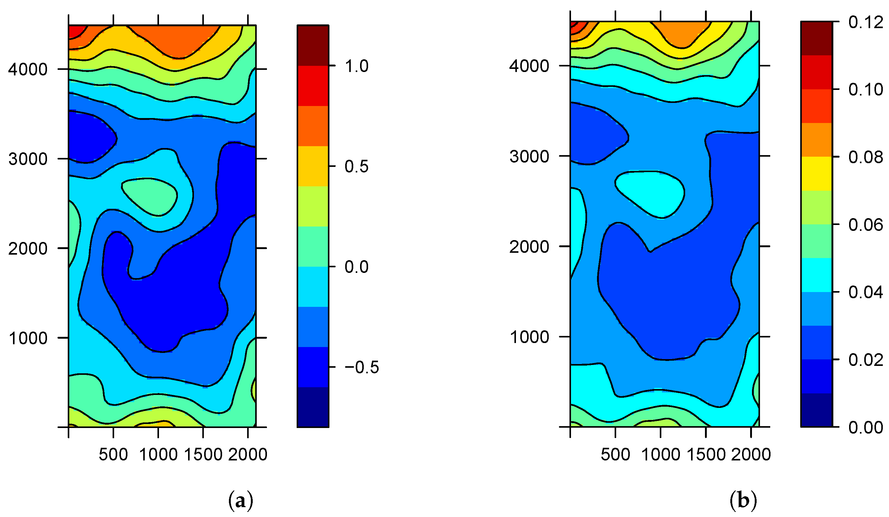
Figure 2a shows the posterior mean of spatial effect
. We observe how the spatial component reaches positive values to the north and south of the nursery, as well as negative values, and achieves values close to zero in the center. In this map, we may recognize the areas with higher risks. This can be explained by the action of the wind that introduces the aphids infected with the virus to the nursery and which carry the disease. The variance in random spatial effect
is equal to 0.13. As the variability takes a small value, we can conclude that the spatial component reflects the pattern of contagion between close saplings located in the same row.
In order to understand the behavior of disease in the nursery, maps were generated with an estimate of the probabilities (
) both at observed sites as well as unobserved sites.
Figure 2b shows the posterior mean probability
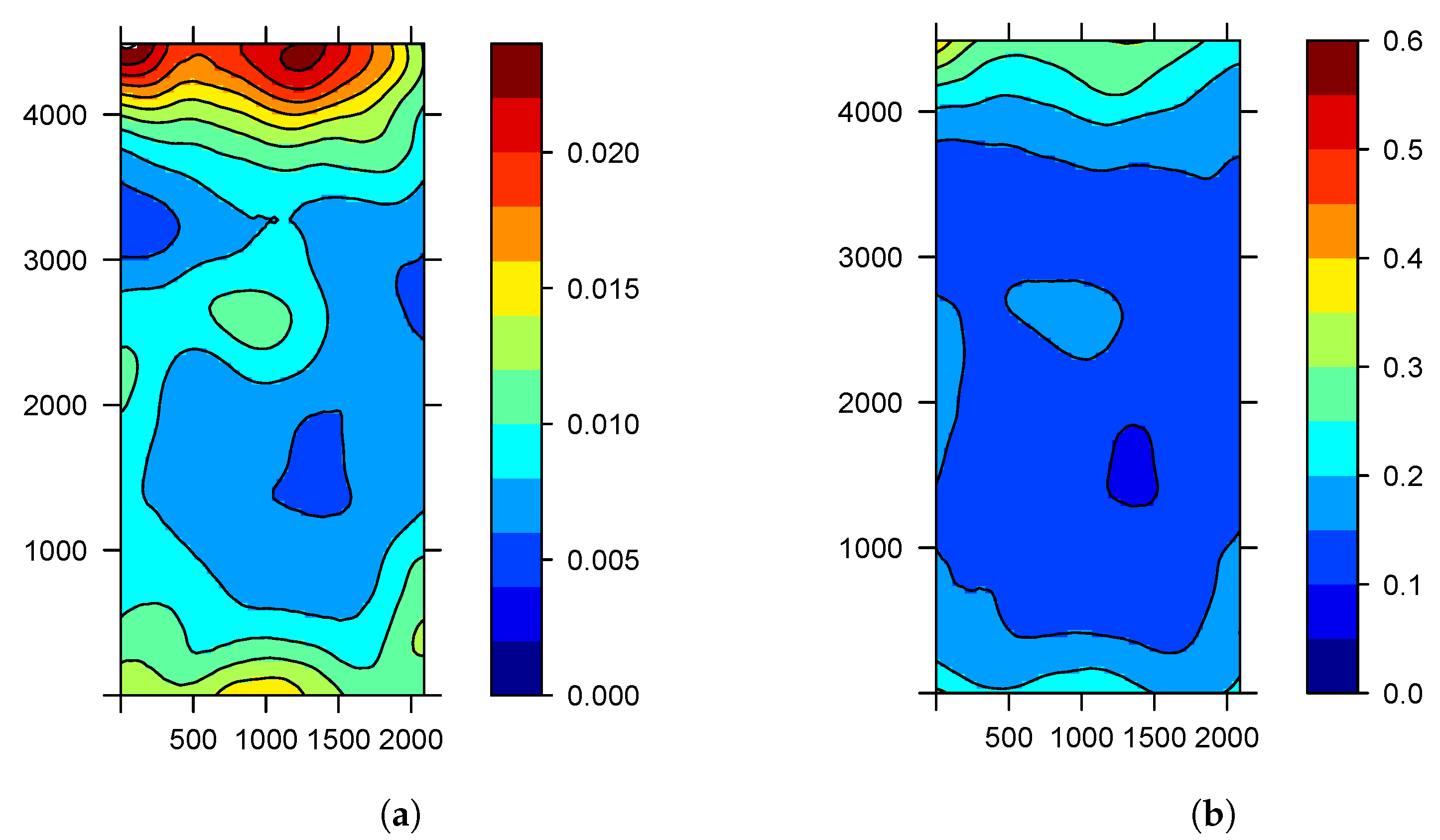
, while
Figure 3a,b shows the quartiles of
. Thus, we obtain not only a point estimate of the probability of the disease of a subject but also an assessment of the uncertainty in this estimate. These figures confirm that the probability of finding the tristeza virus is higher towards the edges of the nursery where the influence of the wind is present.
This type of modeling was used in the context of fisheries, with very good results [
19]. The estimates and results presented in this paper were obtained using the INLA program through the R [
20] package of the same name [
21].


