1. Introduction
Ground stress is the inherent force that causes deformation and even breaking of surrounding rock during tunnel construction without proper design. It seriously affects the regional stability of strata. Many engineering geological disasters, such as large deformation of soft rock section and rockburst of hard rock section, are related to the initial ground stress of stratum rock mass [
1]. Therefore, to ensure the safe construction of the tunnel, it is necessary to test the initial ground stress in the construction area before the construction of large-scale projects such as the tunnel. In most cases, on-site measuring methods, such as the mechanical and vibrating wire load sensors, the hydraulic fracturing and so on, are one of the most advanced and effective methods to obtain the initial ground stress [
2,
3,
4,
5,
6,
7,
8,
9,
10].
Considering the input cost of economy and manpower, it is generally impossible to set up boreholes with sufficient density to fully determine the ground stress in the tunnel area, and the data of the measuring points are discrete and lack representativeness, so there are many limitations in the measurement of ground stress [
11,
12,
13,
14,
15]. Therefore, under the limited on-site measuring data, through effective calculation and analysis methods, a more accurate ground stress and a wide range of ground stress distribution laws can be obtained, which plays an important guiding role in tunnel route selection, excavation, and construction.
For the limitations of in-situ initial ground stress measurement, many theoretical analysis methods have obtained good results of ground stress inversion. To date, the most widely used ground stress inversion calculation methods [
16,
17,
18] are the lateral pressure coefficient method, neural network method, regression analysis method, and so on. The lateral pressure coefficient method is mainly suitable for areas where the geological tectonism is weak and the terrain is flat [
19,
20,
21]. The neural network method is mainly used to solve nonlinear problems, which is in development. Some scholars have shown the feasibility of its application. Gao and Ge [
22] proposed a new type of evolutionary neural network that the rock mass parameters and the initial ground stress can be determined at the same time. The on-site measuring data of the ground stress around the Longtan Tunnel in China were inversely analyzed. The stability of surrounding rock around the tunnel and the accuracy of the initial ground stress calculated by back analysis are verified by numerical calculation. Jin et al. [
23,
24] inversed the parameters of rock mass and the initial ground stress field in the calculated area with a radial basis function network and improved backpropagation network with a model under a finite difference software. Wang et al. [
25] established a three-dimensional model of the underground powerhouse. The factors affecting the initial ground stress field are analyzed, and the results of numerical simulation are used as test set for training in the network model with radial basis function. Finally, the inversion results of the ground stress field in this area are obtained.
In the above-mentioned practical application, the neural network inverse analysis method shows some shortcomings, such as overtraining, slow convergence, and so on [
26]. Therefore, the overall maneuverability of it is weak. The regression analysis method is a calculation method, that is, based on numerical analysis, according to existing data, the regression relationship between independent variables and dependent variables is established [
27,
28]. Combined with the principle of finite element method and regression analysis method, the rationality and accuracy of ground stress analysis are better. It has been widely used in the study of the initial ground stress field.
Regarding the measured stress data of the Lanjiayan highway tunnel, a multiple regression analysis for distribution characteristic of the initial ground stress field of the whole tunnel with numerical calculation was conducted by Dai et al. [
29]. Based on the measured ground stress data, the multiple regression analysis of the initial ground stress field of Wushaoling tunnel is conducted by Zhao et al. [
30], with a finite element software, and the complex ground stress state, the value and distribution of stress in the affected area are determined. The multiple regression analysis reported previously shows that the inversion result of the ground stress field has a good prediction effect compared with the lateral pressure coefficient method and neural network method. The above application studies are all about the accuracy of ground stress inversion and the analysis of the distribution characteristic of the initial ground stress field. However, in the construction area of a super deep-buried tunnel, the study of the following aspects, the comparison and selection of coefficient estimation methods for multiple linear regression equation of ground stress, and the analysis of the lateral pressure coefficient change are less. The inversion principle of the initial ground stress field, and the comparison, and selection of different coefficient estimation methods are mainly described in this study. Based on a tunnel project in China, the initial ground stress field of the tunnel area is only inverted to obtain the main characteristics of the initial ground stress field with super buried depth. The overall content has not been combined with the relevant references to discuss the possible problems and corresponding preventive measures of the tunnel under the condition of high ground stress caused by super buried depth.
2. Multiple Linear Regression Inversion Principle of Initial Ground Stress Field
Regarding conventional mountain tunnels, the designed depth of the tunnel is large. The surrounding rock of the tunnel area is weak. The geological conditions are complex, and the tectonic action is strong. The poor geology is developed. Especially when the whole tunnel axis passes through several large fault fracture zones, geological disasters, such as landslides and collapses, very easily occur [
31,
32]. For the comprehensive action of the above factors, the ground stress in the tunnel area is complex. To grasp the distribution law of the ground stress field of the tunnel area, understand the stratum environment where the tunnel structure is located, and ensure the safety of tunnel construction and operation, it is necessary to measure the ground stress in the tunnel area [
33]. Due to the limitation of geological topography and the input of material resources and manpower, it is impossible to set up boreholes with sufficient density to fully measure the ground stress in the tunnel area. Through the regression inversion of the ground stress, the distribution law of the initial ground stress field can be grasped as a whole, which can provide some reference for the route selection and construction of the tunnel [
34].
The multiple linear regression of the initial ground stress field is based on the multiple linear regression numerical analysis method, which decomposes the complex geological processes in the formation of ground stress into a variety of simple basic factors acting alone [
35]. Using the superposition principle of elasticity, the results of many basic factors are regarded as independent variables and the ground stress at the corresponding points in the ground stress field is regarded as a dependent variable. Then, a linear relationship between the two variables will be established. The initial ground stress field analysis by using multiple linear regression method is only based on the on-site measured data. The differences of methods and technical operations in the process of obtaining on-site measured data are not taken into account. The main implementation method is shown in
Figure 1.
2.1. Establishment of the Three-Dimensional Geological Model
2.1.1. Determination of the Model Range
In the process of initial ground stress regression inversion, two principles [
35,
36] are generally followed to determine the calculation range: (1) the model calculation range includes all the main areas of the tunnel area, and the main geological structures existing in the area, etc.; (2) the boundary of the model is clear and transparent, and it is best to choose in the ridge or river valley. The former is to make the model contain as much data as possible. The more abundant the measured ground stress data, the more accurate and reliable the curve fitting effect will be. The ground stress field inverted by the model is more consistent with the ground stress field in the actual stratum. The latter is for better positioning of the model, and it is easier to impose a single control condition in the process of numerical simulation.
2.1.2. Determination of Model Boundary Conditions
The formation of in-situ ground stress of rock mass is affected by rock mass density, geological tectonism, topography and geomorphology, groundwater action, crustal temperature, and the mechanical properties of the stratum [
37]. The gravity stress of stratum and geological structures are chosen as the main factors affecting the initial ground stress in this study. The following five different stress fields are selected, and the stress state is simulated and calculated by applying displacement and stress conditions. The following different stress field models do not show the boundary constraints, and only the self-weight stress and tectonic displacement boundary conditions are shown. The boundary conditions that the model should have were added in the actual simulation calculation.
- (1)
gravity stress: the required physical and mechanical parameters of surrounding rock such as unit weight, elastic modulus, Poisson’s ratio, cohesion, and internal friction angle can be extracted from the geological survey report, and the gravity stress field is simulated by applying gravity stress in the Z direction to the model (See
Figure 2a).
- (2)
horizontal tectonic stress in X direction: the horizontal tectonic stress in the X direction of rock mass in the model is simulated by applying normal unit horizontal displacement
Ux to the model boundary parallel to the YOZ coordinate plane (See
Figure 2b).
- (3)
horizontal tectonic stress in the Y direction: the horizontal tectonic stress in the Y direction of rock mass in the model is simulated by applying normal unit horizontal displacement
Uy to the model boundary parallel to the XOZ coordinate plane (See
Figure 2c).
- (4)
shear tectonic stress [
38] in the horizontal plane: horizontal shear tectonic stress is simulated by the two implementations, applying a pair of horizontal displacements
U’x parallel to the X-axis and opposite direction to the model boundary interface parallel to the XOZ coordinate plane and applying a pair of horizontal displacements
U’y parallel to the Y-axis and opposite direction to the model boundary parallel to the YOZ coordinate plane (See
Figure 2d).
- (5)
vertical shear tectonic stress: vertical shear tectonic stress is simulated by applying a pair of vertical displacements
Uz with opposite directions on both sides of the model boundary in the XOZ coordinate plane (See
Figure 2e).
2.2. Multiple Linear Regression of Ground Stress Field
2.2.1. Coordinate Transformation of Ground Stress Measured Results
The geological survey results of the initial ground stress are expressed in the direction of East, West, South, and North and the corresponding dip angle, which do not correspond to the coordinate system of the three-dimensional geological model and cannot be directly substituted into the multiple linear regression model for calculation. Therefore, while using the measured ground stress to carry out multiple linear regression for the equivalent ground stress field of the tunnel, it is necessary to conduct coordinate transformation [
39] on the measured ground stress of the on-site measuring points. The coordinates of the corresponding points in the coordinate system of the three-dimensional geological model can be obtained. Then, decomposing the measured ground stress, nine stress components in the three-dimensional spatial coordinate system are transformed and obtained. While the ground stress measurement is conducted with the hydraulic fracturing method, it is generally considered that the measured vertical stress is the vertical principal stress [
40], that is,
and
. Therefore, the principal stress in the XOY coordinate plane is only needed to decompose in the plane coordinate system.
,
,
and
are accordingly obtained. Taking the due north direction as the polar coordinate X-axis direction, the transformation formula of stress component from polar coordinate to Cartesian coordinate is as follows.
In the formula:
—Radial stress value of initial ground stress at measuring point in polar coordinate system;
—Circumferential stress value of the initial ground stress at the measuring point in the polar coordinate system;
—Shear stress value of initial ground stress at measuring point in polar coordinate system;
θ—The angle between the initial ground stress direction of the measuring point and the x-axis in the polar coordinate system;
—x direction stress component of initial ground stress at measuring point in Cartesian coordinate system;
—y direction stress component of initial ground stress at measuring point in Cartesian coordinate system;
, —Shear stress component of initial ground stress at measuring point in Cartesian coordinate system.
2.2.2. Multiple Linear Regression Equation
According to the principle of the multiple linear regression method [
41], taking the calculated value of initial ground stress corresponding to the on-site point under different boundary conditions as the independent variable and the calculated value of ground stress regression as the dependent variable, the regression calculation equation is obtained as follows.
In the formula:
—initial ground stress calculation value of stress component j at measured point k;
, —undetermined coefficient in multiple linear regression equation;
n—number of boundary conditions, five working conditions are discussed in this study;
—in-situ ground stress component caused by the gravity stress mode and each sub tectonic stress mode, respectively.
In the formula:
—initial ground stress measured value of stress component j at measured point k;
—the error between the in-situ value of initial ground stress and the calculated regression value, which obeys normal distribution and is independent of each other.
To maximize the fitting degree of the multiple linear regression curve and obtain the regression equation that can best reflect the actual ground stress field, it is necessary to minimize the sum of total deviation squares between the measured data and the regression calculation data while minimizing the sum of the regression squares. Assuming the number of on-site measured points is
n, and the stress state of a point in the area is represented by 6 stress components. The following calculation equation for the sum of total deviation squares
, the sum of regression squares
, and the sum of residual squares
can be obtained. See Equations (4)–(6):
Following calculating the partial derivative , its partial derivative is made equal to zero, and the normal Equation (7) for calculating the regression coefficient are obtained.
2.2.3. Determination Method of the Regression Coefficient
Based on the diversity of coefficient estimation methods for multiple linear regression, the ordinary least square method (OLS), ridge regression (RR), and lasso regression (LR) are selected to estimate the coefficients of the regression equation. The regression fitting results are compared and selected. To achieve the best fitting effect, the coefficients of each fitting method are estimated based on minimizing the sum of residual squares of the fitting values, and the main principles are shown in
Table 1.
2.2.4. Regression Effect Test
To judge the regression effect of the regression equation on the measured ground stress, it is necessary to test its significance, and to judge whether the calculated value of ground stress regression as a dependent variable has a significant multiple linear relationship with the calculated value of the initial ground stress corresponding to the measured points under different boundary conditions. The insignificant factors should be eliminated, and then the inversion calculation should be carried out again. For the comparison and selection of the subsequent regression equations of the initial ground stress field, the regression results using different coefficient estimation methods are compared. The test method used is shown in
Table 2.
3. Case Study
3.1. Measured Results of In-Situ Stress in the Tunnel Area
The maximum burial depth of a tunnel in China is 1100 m. There are 8 tunnel sections with a buried depth of more than 500 m, a total of 10,055 m. Two sections with a buried depth of more than 800 m, is a total of 3885 m. During the measurement, the in-situ stress test was carried out on 13 holes along the tunnel line, and the test method was the hydraulic fracturing method. Each measuring point is tested at the bottom of the hole, and the test range of the hole depth is 91 m~946 m. The area that the tunnel passes through is dominated by V-class surrounding rocks with poor mechanical properties [
44]. The relatively complete area is mixed with grade IV-class surrounding rocks [
44].
The maximum horizontal principal stress is in the range of 8.08~35.25 MPa, the minimum horizontal principal stress range is in the range of 7.46~20.86 MPa, and the vertical principal stress range is in the range of 4.79~23.93 MPa. In hole 9, the maximum value of maximum horizontal principal stress (35.25 MPa) and the maximum value of minimum principal stress (20.86 MPa) are measured at the same time, and the vertical principal stress is 22.69 MPa. In hole 1, the minimum value of maximum horizontal principal stress (8.08 MPa) and the minimum value of minimum principal stress (7.46 MPa) are measured at the same time, and the vertical principal stress is 4.79 MPa. According to the analysis of the test results, the ground stress increases linearly with the increase of the hole depth. The magnitude relationship of the three principal stresses is as follows (from large to small): maximum horizontal principal stress, minimum horizontal principal stress, and vertical principal stress, indicating that the ground stress in the tunnel area is mainly horizontal tectonic stress.
3.2. Establishment of FLAC 3D Model
The length × width of the model is 21,000 m × 7600 m. The height of the highest point of the model is 5065 m from the bottom, and the trend of the tunnel is roughly parallel to the X-axis. The whole model is extended according to the actual contour map of the tunnel area, which can reflect its topographic and geomorphological features. The model includes the fault structural zone along the tunnel. Boundary condition of the numerical model is shown in
Table 3. The physics and mechanical properties of rock mass are shown in
Table 4. The fault is dominated by tectonic breccia. All parameters are determined by laboratory and field tests, all of which follow the relevant specification [
45]. The FLAC 3D model is shown in
Figure 3. The model uses Midas GTS/NX software to divide the grid, in which the maximum grid size is 100 m and the number of elements is 4087841. For the numerical simulation analysis with FLAC 3D software, the mechanical properties of the material follow the elastic constitutive model. The mechanical properties of materials are presented in terms of the mechanical properties of the rock mass from the site.
3.3. Coefficients Determination of Regression Equation
According to the selected five boundary constraint conditions and the distribution of 13 on-site measured points, the established three-dimensional geological model is numerically simulated, and the theoretical values of stress components at 13 corresponding measuring points of model are obtained. To verify the reliability of the inversion results of the ground stress by the multiple linear regression, the calculated data of measuring points 1 and 2 are retained not to participate in the regression fitting calculation. Based on the calculation results of the three-dimensional geological model under five boundary conditions, each component of the ground stress at the corresponding point of the model is taken as the regression target value. The application of three linear regression coefficient estimation methods is realized by using Python code, and the multiple linear regression coefficients of each group are obtained as shown in
Table 5. The multiple linear regression equation of the initial ground stress field in the tunnel area is obtained as Equations (8)–(10).
The equations with different coefficient estimation methods are as follows.
In the formula:
—the stress component of a point in the equivalent stress field calculated by the model;
—the stress component of a point under the independent action of the gravity stress field calculated by the model;
—the stress component of a point under the independent action of horizontal squeezing stress in the X direction calculated by the model;
—the stress component of a point under the independent action of horizontal squeezing stress in the Y direction calculated by the model;
—the stress component of a point under the independent action of shear stress in the XOY coordinate plane calculated by the model;
—the stress component of a point under the independent action of shear stress in the XOZ coordinate plane calculated by the model.
It should be noted that the components represented by , , , , and correspond to , and the equation should be substituted into the calculation in kPa.
3.4. Regression Results Analysis of Initial Ground Stress
3.4.1. Significance Test of Regression Analysis
The significance test of the regression analysis results obtained by the three coefficient estimation methods is shown in
Table 6.
As can be seen from
Table 6, in the significance test results of the regression equation obtained by the three coefficient estimation methods, the multiple correlation coefficient is close to 1.0, and the fitting effect is good. According to the F test distribution table,
. Compared with the results of the significance test, under the condition that the confidence degree of significance level reaches 95%, there is a very significant linear relationship between the dependent variable “ground stress component regression calculated value” and the independent variable “the calculated value of initial ground stress component corresponding to the measured point under different boundary conditions”. The fitting result of the multiple linear regression equation of the initial ground stress is reliable. It can be seen from D-W = 1.88 that there is only slight multicollinearity among the sample variables selected for regression analysis, while the statistics are close to 2.0, so it can be considered that the sample variables are independent of each other. The significance test results of OLS and LR analysis are the same. Therefore, considering the multicollinearity between variables and the unbiased estimation of regression fitting values, the coefficient estimation of the initial ground stress field regression equation is conducted and extended by the lasso regression method in the follow-up case.
3.4.2. Comparison between Regression Fitting Value and On-Site Measured Value
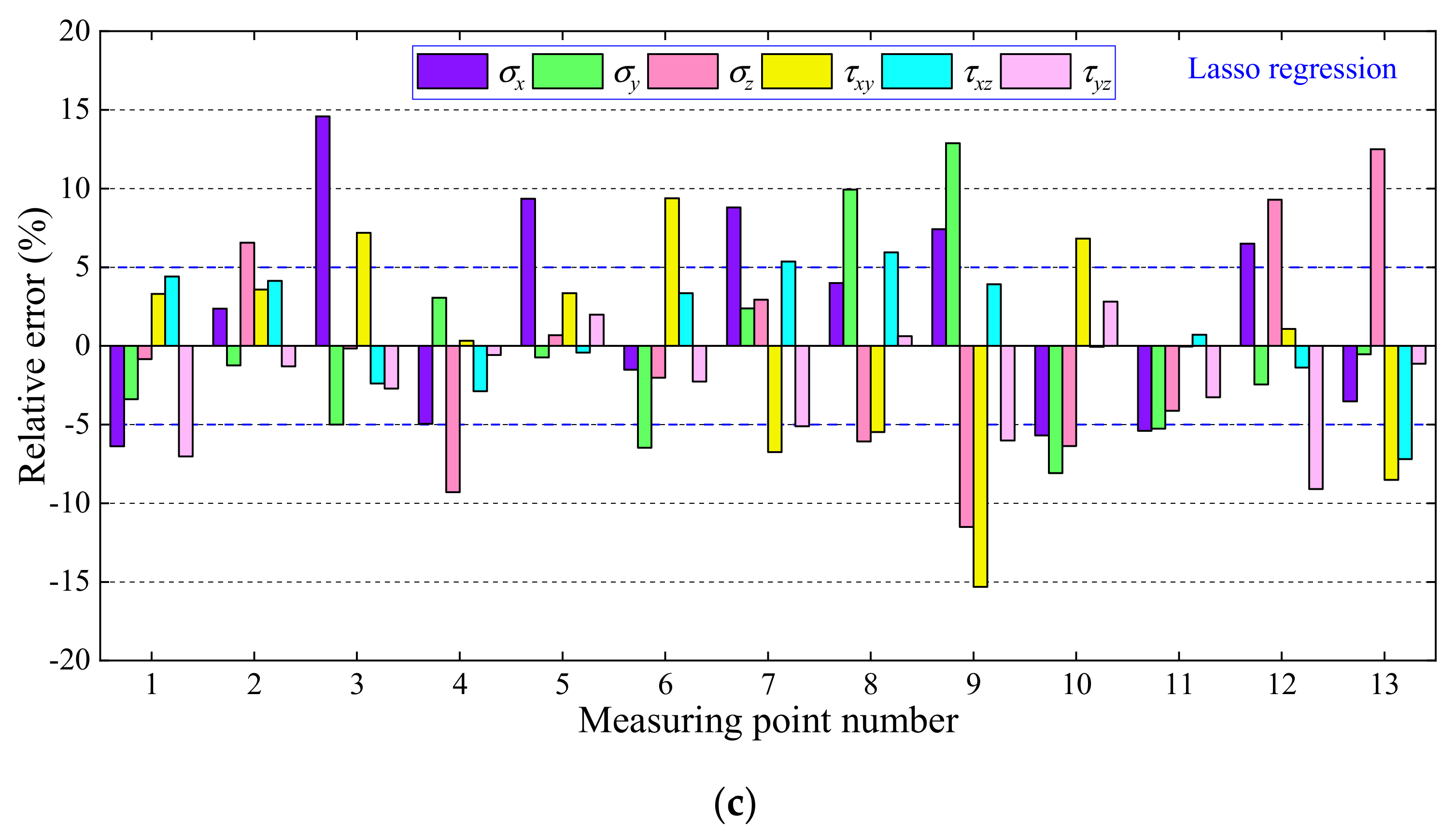
According to the multiple linear regression equation and the calculation results of the ground stress field of the three-dimensional geological model under each boundary condition, the regression calculation value of each stress component at each extracted point is obtained. The difference between the regression value and the measured value is called the relative error for the ground stress. The relative errors of ground stress inversion results at 13 measuring points are shown in
Figure 4. The comparison of regression results of the three coefficient estimation methods is shown in
Table 7.
From the analysis of
Figure 4, it can be seen that, including the samples of point 1 and point 2 which are not involved in the regression calculation, under the three coefficient estimation methods, most of the absolute value of relative errors between the measured values and the regression values of initial ground stress are controlled within 10%. Among them, there are only 6 data exceeding 10% under the OLS method and only 5 data exceeding 10 % under the LR method, accounting for 6.4% of all statistics. Meanwhile, the fluctuation of the absolute value of relative error is small, and the average value of the ridge method is the largest, at 4.99%. The mean relative error of OLS is close to that of LR, and the minimum is 4.73% with the OLS method, which indicates that the values of regressed and measured are relatively close. The regression fitting result of the ground stress is reasonable and reliable, which can well reflect the distribution of the initial ground stress field in the tunnel area. To sum up, when considering the small relative error, the OLS method is very close to the LR method, and the relative error of the LR method is less regarding the larger data value, which shows that the LR method has a good effect on the regression fitting of the initial ground stress field.
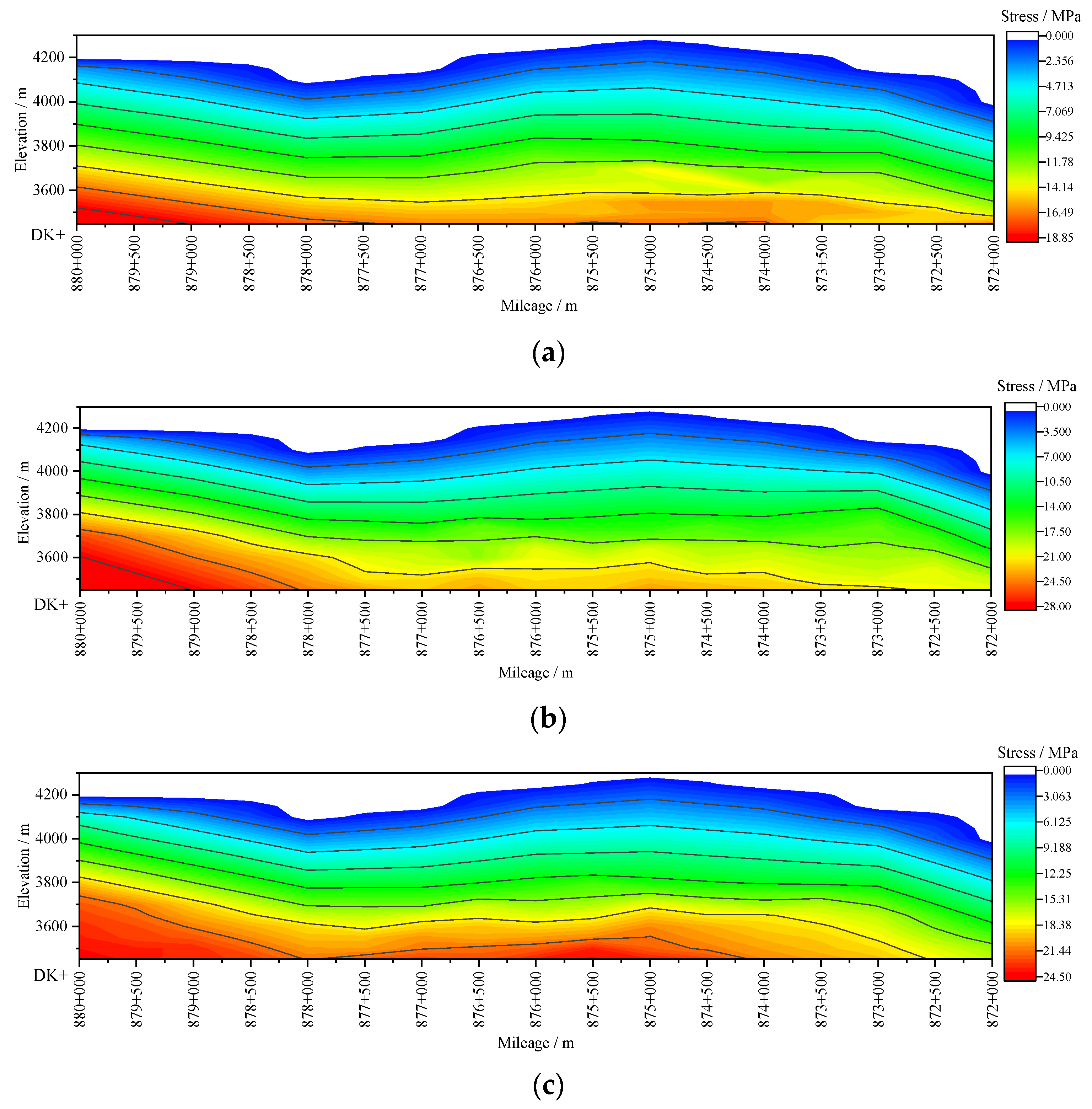
3.5. The Inversion Results Analysis of Initial Ground Stress
Using the calculation results of each stress component of different stress states in the 3D geological model, combined with the multiple linear regression equation, the ground stress nephograms at different depths of the longitudinal section along the tunnel in China are finally calculated, as shown in
Figure 5. To explore the distribution of the initial ground stress field of the surrounding rock around the tunnel, the initial ground stress data of 500 m, 800 m, and 1100 m were extracted from the mileage section DK872~DK880 with large depth fluctuations of the tunnel, respectively. Nine points were extracted for each type of buried depth, and the measuring point interval is 1000 m. Using the multiple linear regression equation of the initial ground stress field, the stress components of different stress states in the three-dimensional geological model were superimposed and calculated. The principal stress at the extraction point is obtained as shown in
Table 8.
According to the analysis in
Table 8, the lateral pressure coefficient of the tunnel line area gradually decreases with the tunnel buried depth increasing. The lateral pressure coefficient in the direction of large horizontal principal stress with a buried depth of 500 m ranges from 1.5 to 1.8, and the lateral pressure coefficient in the direction of small horizontal principal stress ranges from 1.1 to 1.5; The lateral pressure coefficient in the direction of large horizontal principal stress with a buried-depth of 800 m ranges from 1.3 to 1.5, and the lateral pressure coefficient in the direction of small horizontal principal stress ranges from 1.1 to 1.3; The lateral pressure coefficient in the direction of horizontal large principal stress with a buried depth of 1100 m ranges from 1.2 to 1.3, and the lateral pressure coefficient in the direction of horizontal small principal stress ranges from 1.0 to 1.1.
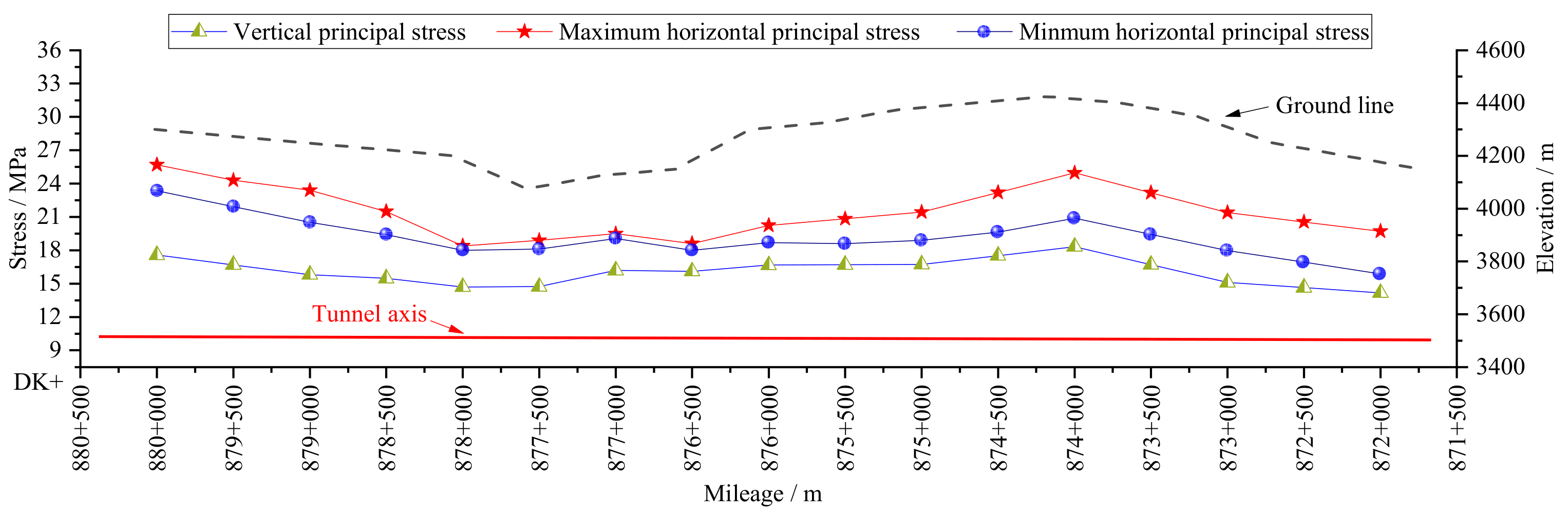
Further extracting the stress value, the relationship between the principal stress value and mileage at the tunnel axis is obtained, as shown in
Figure 6.
From
Figure 5 and
Figure 6, it can be seen that the distribution characteristics of the stress field along the tunnel are closely related to the topographic. When the topographic relief increases, the stress isoline density increases, and the ground stress change gradient increases, which is consistent with the distribution characteristic of the actual ground stress field. The maximum vertical principal stress along the tunnel is 18.3 MPa, which is about at the mileage of DK874+000. The maximum value of the maximum horizontal principal stress is 26.8 MPa, which is about at the mileage of DK880+000; The maximum value of the minimum horizontal principal stress is 23.3 MPa, which is about at the mileage of DK880+000. The overall stress characteristics from large to small are as follows: the maximum horizontal principal stress, the minimum horizontal principal stress, and the vertical principal stress, which indicates that the horizontal tectonic stress is dominant in the tunnel area and the horizontal tectonic stress is significant. Compared with the uniaxial compressive strength of the rock mass in
Table 4, the ratio of surrounding rock strength to the ground stress is less than 0.5, indicating that the ground stress is high and prone to large deformation [
44]. There is F3 fault at the tunnel mileage of DK878+000. The horizontal tectonic stress is slightly released [
32], and the ratio of horizontal principal stress to vertical principal stress is smaller than that of both sides. The reduction of the geo-tress at the fault makes the stress of the tunnel structure uneven, which is very disadvantageous to the tunnel structure. At this time, the structure needs to be strengthened, and the adaptive implementation of support becomes inevitable [
46]. F2 fault also exists at the tunnel mileage of DK876+500, and the regional tectonic stress is partially released [
32]. The ratio of horizontal principal stress to vertical principal stress of the adjacent area shows the same trend. The trend is different from the analysis results of the lateral pressure coefficient beyond the fault, indicating that the influence of fault fracture zone on ground stress is significant. It can be seen that the lateral pressure coefficient in the super deep and super high ground stress area must be determined only by a more thorough investigation and an on-site test. It can be seen that the inversion results of in-situ ground stress need to be verified by more on-site measured results, and the accuracy and precision of the inversion results have a large room for improvement. The algorithm solution of the analysis and inversion application for the corresponding in-situ ground stress field law is very meaningful.


