Roll Eccentricity Signal Detection and Its Engineering Application Based on SFFT-IAA

Abstract

The roll eccentricity signal is a weak and complex periodic signal that is difficult to be identified. To improve the detection accuracy of the roll eccentricity signal and to compensate effectively, this study proposed a roll eccentricity signal detection method by combining the sparse fast Fourier transform (SFFT) and the iterative adaptive approach (IAA). The proposed method can rapidly determine the frequency range of the roll eccentricity signal by using the SFFT. Then, it divides the frequency range into several small frequency bands. In each small frequency band, the frequency, amplitude, and phase angle of each harmonic component of the roll eccentricity signal were estimated by using IAA. The simulation results show that the proposed method can find all frequency components, and the frequency estimation accuracy is higher than 99.88%. Finally, the engineering application of this method and the eccentricity compensation control were investigated. In engineering applications, the proposed method can reduce the thickness fluctuation of the finished strip by 89.2%, and the product quality is improved significantly. The simulation results and engineering experiments show that the proposed method has an excellent effect on detecting and compensating roll eccentricity signals.

1. Introduction

The roll eccentricity can be observed in various rolling mills for plates and strips, and it is a dominant factor affecting the quality of finished strip steels in modern high-precision and high-speed cold-rolling strip steel production. Roll eccentricity can lead to the high-frequency vibration of rollers during high-speed rotation, thus resulting in periodic oscillations in the practical roll gap of the rolling mill and causing periodic fluctuations in the thickness of the finished strip steels. In engineering practice, roll eccentricity is unavoidable, and the quality of finished strip steels can only be ensured by the rolling mill control system and its control methods. The automatic gauge control (AGC) system is commonly used in cold rolling mills, but its main thickness control methods (feedforward AGC, feedback AGC, and mass flow AGC) cannot suppress the thickness fluctuations caused by roll eccentricity. Such thickness fluctuations can cause the AGC system to suffer from reverse regulation, thus reducing control quality and seriously affecting the quality of the finished strip steels [1]. At present, with the increasing demand for high-quality, high-yield, and low-cost rolling strip steels, it is urgent to effectively compensate for roll eccentricity. The basic idea of roll eccentricity compensation is to establish a roll eccentricity model by extracting the roll eccentricity signal from the data containing the eccentricity information, such as roll gap, rolling force, tension, or thickness deviation. Then, the proposed eccentricity model is used to obtain the eccentricity compensation signal, and the obtained signal is fed into the hydraulic servo position control system of the rolling mill to compensate for the fluctuations of the roll gap caused by the roll eccentricity, thus reducing the strip steel thickness error caused by the roll eccentricity.

According to the mechanical structure and the operating characteristics of rolling mills and rollers, the following aspects should be considered in roll eccentricity compensation:

• A roll eccentricity signal is a complex high-frequency periodic signal mixed with random disturbances and containing multiple harmonics. In addition, the signal is featured with periodicity, variability, complexity, and weakness and cannot be measured directly [2].
• The frequency of eccentricity signals changes with the rolling speed, so the detection of eccentricity signals must be quick and be adaptable to the changes in the parameters of eccentricity signals.
• The same types of rollers (such as upper and lower backup rollers and work rollers) have different but close roll diameters and the frequencies of the harmonic components of their eccentricity signals will be very similar.
• The roll diameters of different types of rollers differ greatly and the frequencies of the roll eccentricity signals vary in a wide range.

From the above analysis, it can be seen that the detection of the roll eccentricity signal is very difficult. First, the eccentricity signal is weak. In the collection of signals containing the eccentricity information, the eccentricity part accounts for a small proportion and it is easily affected by interference signals. Second, the roll eccentricity signal has very similar frequency components and it is difficult to distinguish completely by the commonly used signal process methods under the interference of noise. Furthermore, the roll eccentricity signal cannot be directly measured by the sensors and must be obtained by the method of soft measurement. If the eccentricity signal cannot be detected accurately, the eccentricity compensation control will not only fail to improve the product quality but even cause the deterioration of the product quality.

Therefore, rapid and accurate detection of the amplitude, frequency, and initial phase angle of eccentricity signals from complex signals obtained by establishing the corresponding mathematical model are key to compensating and controlling roll eccentricity. The roll eccentricity signal is generated by a series of nonlinear periodic signals with different frequencies superimposed on each other. To detect roll eccentricity signals, scholars have conducted extensive research and made certain achievements. As a simple and effective method in digital signal processing, FFT and the improved FFT-based algorithms have been applied for the detection of eccentricity signals [3]. Due to a low resolution, FFT is only applicable when the sampling period is an integer multiple of the eccentricity signal components; however, this condition cannot be satisfied in the rolling process. In this case, spectral leakage and fence effect will occur. Compared with FFT, wavelet transform has good localization characteristics in the time and frequency domains, and some studies used wavelet analysis to extract roll eccentricity signals [4,5]. However, since the performance of wavelet analysis depends on the selection of the wavelet basis function, frequency overlap tends to occur when detecting similar harmonic frequencies and there is a high calculation amount with large redundancy. Yang Qiu-xia et al. [6] proposed a neural network-based method for processing eccentricity signals. However, the neural network has a low resolution and a long learning time and is easy to fall into local minima, resulting in low performance in distinguishing similar frequencies. In recent years, some new methods have been applied to eccentricity signal detection. Li Feng-ji et al. [7] also used the RBF neural network to extract the roll eccentricity signal and, by using POS to optimize the parameters of the RBF, the accuracy and speed were improved compared with the traditional neural network method. Li Zhong-de et al. [8] proposed an ensemble empirical mode decomposition (EEMD) method for eccentricity signal extraction. The method can be applied to distinguish similar frequencies in eccentricity signal components, but its performance depends on the amplitude of the adaptive added noise and the selection of the ensemble number in EEMD. In practical applications, it is crucial to properly set the two parameters. Wei Lixin et al. [9] also used the EEMD algorithm, but first used the wavelet threshold method to denoise the roll eccentricity disturbance signal. Liu Tao et al. [10] proposed a method for roll eccentricity signal analysis based on the resampling method with computed order tracking, which can solve the problems of frequency overlap and frequency change due to the change in the rolling speed. However, in this method, phase detection signals are obtained by data fitting and original signals cannot be reconstructed, thus it is difficult to guarantee the accuracy of the constructed eccentricity model. Wang Hong-xi et al. [11] proposed a method for detecting roll eccentricity signals based on the high-order cumulant-based Root-MUSIC method and Prony method. The proposed method performed well in frequency resolution and noise immunity and the accuracy of the reconstructed eccentricity model was also high. From the perspective of engineering applications of roll eccentricity compensation, Hao Luo et al. [12] developed an adaptive observer to estimate the eccentricity signal frequency for a single supporting roll eccentricity. Then, the amplitude and frequency of eccentricity signals were estimated by an adaptive algorithm based on normalized gradient. Xu Xiang-Yu and Li Hai-long [13] proposed a multiple modulation zoom spectrum analysis for estimating the frequency and the amplitude of roll eccentric harmonics and the phase angle of the roll eccentric harmonics were estimated by FFT. Gao SF et al. [14] used wavelet analysis that determined a reasonable threshold by MPSO algorithm to first denoise the signal. Then, the roll eccentricity signal was extracted from the denoised signal by decomposition into proper rotational components using the intrinsic time-scale decomposition.

Considering the above characteristics of roll eccentricity signals and from the perspective of practical applications, this paper proposed a roll eccentricity detection method by combing the iterative adaptive approach (IAA) and the sparse fast Fourier transform (SFFT). IAA is a nonparametric spectral estimation method proposed by Li in recent years [15]. This method has the advantages of high frequency resolution, high noise immunity, and high robustness. It can be used to solve the frequency overlapping problem. In addition, it is applicable in the case of a small amount of data and is simple and easy to implement. For this reason, the IAA method has been widely used in array signal processing, underwater communication, image processing, and other fields [16,17,18]. However, the resolution of IAA is proportional to the calculation amount. In the rolling production process, the rolling speed varies widely and the frequency of the roll eccentricity signals changes in a wide range. In this case, the use of IAA for a highly accurate detection of eccentricity signals will lead to a very high calculation amount and cannot meet the requirements for real-time performance. Considering that the roll eccentricity signal is a typical sparse signal, this paper used SFFT to investigate the frequency distribution of each harmonic of roll eccentricity signals and then set several small frequency bands according to the frequency distribution. In each small frequency band, IAA was used to accurately detect the signals to construct an accurate roll eccentricity model. The simulation results and the engineering experiments indicated that the proposed method can guarantee the accuracy of eccentricity signal estimation, meet the requirements for real-time performance, and show a good compensation effect, which has a high application value in engineering fields.

The major contributions of this paper are as follows:

• On the problem of roll eccentricity signal detection, the IAA algorithm is improved by using SFFT, and SFFT-IAA is proposed.
• The similar frequency components in the roll eccentricity signal can be detected. A high precision roll eccentricity compensation model is established.
• The application method of roll eccentricity signal detection in engineering is discussed.

The remainder of this paper is organized as follows: Section 2 discusses the related problems of roll eccentricity of a cold rolling mill and gives a mathematical model of the eccentricity signal. Section 3 is a fine description of SFFT-IAA. Section 4 is a simulation study to verify the performance of SFFT-IAA. Section 5 introduces the application and verification of the proposed method in the actual single-stand reversible cold rolling mill. Section 6 contains some conclusions.

2. Description of Roll Eccentricity Problems

Currently, the roller system of the mainstream single-stand reversible cold rolling mill consists of six rollers of different diameters. In the rolling process of plates and strips, the rollers are pressed against each other under the rolling force generated by the hydraulic cylinder and are rotated at a high speed driven by the motor drive system. Then, the AGC system changes the size of the roller gaps by adjusting the position of the hydraulic cylinder to obtain the thickness of the exporting strip steel. Figure 1 illustrates the working principle of the six-roller reversible cold rolling mill.

According to the spring equation for rolling mills, the exit thickness of the strip steel is [19]:

$$h=S_0+\frac{P}{M}$$

(1)

where $h$ is the exit thickness of the strip steel, $S_0$ is the unloaded roller gap, $P$ is the rolling force, and $M$ is the stiffness of the rolling mill. It can be deduced from Equation (1) that the exit thickness fluctuation $\Delta h$ after thickness control is:

$$\Delta h=\frac{\Delta P}{M_C}$$

(2)

$$M_C=\frac{\partial P}{\partial h}=M\left(1-C\right)$$

(3)

where $M_C$ is the effective stiffness of the rolling mill, $\partial P$ is the fluctuation of the rolling force, $\partial h$ is the thickness deviation of the rolled piece, and $C$ is the compensation coefficient at the position of the roller gap.

$$\Delta P=\left(\Delta H-\Delta h\right)Q$$

(4)

where $\Delta H$ is the entry thickness of the rolled piece, and $Q$ is the plastic stiffness. If the roller eccentricity amount $e$ is considered, Equation (2) can be rewritten as:

$$\Delta h=e+\frac{\left(\Delta H-\Delta h\right)Q }{M_C}$$

(5)

Then, we have:

$$\Delta h=\frac{ M_C}{M_C+Q}e+\frac{Q }{M_C+Q}\Delta H$$

(6)

When the common thickness gauge control method is used in the thickness control system, the value of $C$ ranges from 0 to 1, the value of $M_C$ ranges from $M$ to $\infty$, and the roll eccentricity $e$ will be nearly or even completely reflected in the thickness deviation of the rolled piece, which cannot be eliminated. Figure 2 illustrates the impacts of roll eccentricity.

As shown in Figure 2, when eccentricity $e$ exists, the actual thickness of the strip decreases by $\Delta h_e$ and the rolling force increases by $\Delta P_e$. In this case, the control system considers that the thickness of the strip increases. Therefore, under the action of the controller, the system operates in the direction of reducing the thickness of the strip, which leads to a low thickness accuracy and deteriorated control quality. In actual situations, when roll eccentricity exists, the roller will vibrate at a high frequency during high-speed rotations, resulting in periodic oscillations in the practical roll gap of the rolling mill, rolling force, and thickness of the exit strip steel.

Roll eccentricity can be divided into two main types: the rotational eccentricity generated when the center of rotation of the roller does not coincide with its geometric center and the elliptical eccentricity caused by the irregular shape of the roller itself. In engineering practice, both types of roll eccentricity may exist. According to the causes of roll eccentricity and the working mechanism of rolling mills, the unified model of roll eccentricity can be expressed as the superposition of a series of cosine periodic waves obtained by integer multiples of the roller rotation. Thus, the frequency of an eccentricity component induced by the rotational eccentricity is the same as the rotational frequency of the roller, and the frequency of the eccentricity component of the roller caused by ellipticity is two times the rotation period [20]. Therefore, the eccentricity signal model can be expressed as:

$$y\left(n\right)={{\displaystyle \sum }}_{i=1}^k{A}_{i}cos\left({\omega }_{i}n\Delta t+{\phi }_i\right)+v\left(n\right)$$

(7)

where $y\left(n\right)$ is the sampling value of the eccentricity signal, $k$ is the number of harmonic components, i.e., the sparsity of the eccentricity signal, $A_i$ is the amplitude of the $i$th eccentricity signal, ${\omega }_i$ is the angular frequency of the $i$th eccentricity signal, $n$ is the number of samples, $\Delta t$ is the sampling period, and ${\phi }_i$ is the initial phase angle of the $i$th eccentricity signal. $v\left(n\right)$ is a random noise, whose amplitude distribution follows a Gaussian distribution and whose power spectral density follows a uniform distribution, i.e., white Gaussian noise. Moreover, it should be pointed out that the method proposed in the following sections needs to use the least squares estimation, whose premise is that the noise satisfies the Gaussian distribution.

An accurate eccentricity model can be established based on the frequency ${\omega }_i$, amplitude $A_i$, initial phase angle ${\phi }_i$, and other parameters of each harmonic of the above eccentricity components, thus achieving the compensation and control of eccentricity.

3. Roll Eccentricity Signal Detection Based on SFFT-IAA

3.1. Detection of Eccentricity Signal Parameters Based on IAA

The characteristics of eccentricity signals determine the difficulties in eccentricity signal detection, i.e., effectively suppressing the effects of various random interferences and achieving a high enough resolution. However, these difficulties are hard to overcome by conventional signal detection methods. For IAA, since it has a high frequency resolution and each frequency component is solved one by one, all other components are regarded as noise in solving a frequency component, thus avoiding the influences of random interferences and other components. Meanwhile, the resolution is a parameter in the calculation process, and a high enough resolution is needed. Additionally, by using IAA, the frequency, amplitude, and phase angle of a signal can be obtained at the same time, which simplifies the calculation process compared with the conventional methods. Hence, the use of IAA can meet the requirements of good interference resistance and high resolution for eccentricity signal detection.

According to Equation (7), an eccentricity signal is generated by the superposition of a series of cosine signals with different frequencies; each frequency component in cosine form can be decomposed into the sum of a sine signal and a cosine signal. Thus, Equation (7) can be rewritten as:

$$y={{\displaystyle \sum }}_{i=1}^k{D}_i{\alpha }_i+v$$

(8)

where

$$D_i=\left[c_i,s_i\right],{\alpha }_i={\left[a\left({\omega }_i\right),b\left({\omega }_i\right)\right]}^T$$

$$c_i^T=\left[cos\left({\omega }_i\Delta t\right),\cdots , cos\left({\omega }_{i}n\Delta t\right)\right]$$

$$s_i^T=\left[sin\left({\omega }_i\Delta t\right),\cdots , sin\left({\omega }_{i}n\Delta t\right)\right]$$

$$v^T=\left[v\left(1\right),\cdots , v\left(N_I\right)\right]$$

$$\left(i=1,2,\cdots ,k\right)$$

Based on the measurable data containing the eccentricity information (e.g., rolling force, roller gap, and thickness deviation), a numerical sequence of length$N_I$ can be measured; it is denoted as $y$:

$$y^T=\left[y\left(1\right),\cdots , y\left(N_I\right)\right]$$

(9)

Let the frequency range of eccentricity signals be $\left[{\omega }_{min},{\omega }_{max}\right]$. Within the frequency range, a set of virtual frequency grids is generated with a frequency spacing of $\Delta \omega$. Obviously, the number of generated grids is:

$$m=1+\frac{{\omega }_{max}-{\omega }_{min}}{\Delta \omega }$$

Therefore, the frequency of each grid is ${\omega }_j={\omega }_{min}+\left(j-1\right)\Delta \omega , j=1,2,\cdots ,m$.

The overall framework of the IAA algorithm is shown in Algorithm 1.

Algorithm 1: The overall framework of IAA

Input: The numerical sequence of length $N_I$. Output: A set of the frequencies of the harmonics and the amplitudes. 1   Initialize IAA parameters; 2   Initialize the amplitudes corresponding to the frequency of each virtual grid by the basic least squares; 3   Set the number of iterations to 0; 4   While maximum number of iterations is not reached do 5          for $j$ = 1: $m$ do 6              Calculate the amplitude of ${\omega }_j$ by the weighted least squares; 7          end 8          number of iterations = number of iterations + 1; 9   end 10   for $j$ = 1 : $m$ do 11             Calculate the power spectrum of ${\omega }_j$; 12   end 13   Search for the top $k$ peak values in the power spectrum.

According to the principle of the least squares method, the objective function at the $j$th frequency grid is $min\left(\Vert y-D_j{a}_j{\Vert }_j^2\right)$. Then, we have:

$$\widehat{ a_j}={\left(D_j^T{D}_j\right)}^{-1}{D}_j^{T}y$$

(10)

To avoid the interferences between different frequency components, in solving a grid frequency, the other grid frequencies are considered as noise. Therefore, in the iteration process, the weighted least squares method is employed to solve the objective function. According to the weighted least squares method, the objective function can be written as:

$$min\left[{\left(y-D_j{a}_j\right)}^T{Q}_j^{-1}\left(y-D_j{a}_j\right)\right]$$

(11)

where $Q_j$ is the covariance matrix in solving the $j$th frequency component and it can be expressed as:

$$Q_j=R-D_j{A}_j{D}_j^T$$

(12)

$$A_j=\frac{a^2\left({\omega }_j\right)+b^2\left({\omega }_j\right)}{2}\left[\begin{array}{cc}1& 0\\ 0& 1\end{array}\right]$$

(13)

$$R={{\displaystyle \sum }}_j^m{D}_j{A}_j{D}_j^T$$

(14)

According to the weighted least square method, we have:

$$\widehat{a_j}={\left(D_j^T{Q}_j^{-1}{D}_j\right)}^{-1}\left(D_j^T{Q}_j^{-1}y\right)$$

(15)

The inverse of $Q_j$ can be obtained by:

$$Q_j^{-1}={\left(R-D_j{A}_j{D}_j^T\right)}^{-1}=R^{-1}+R^{-1}{D}_j{A}_j{\left(I-D_j^T{R}^{-1}{D}_j{A}_j\right)}^{-1}{D}_j^T{R}^{-1}$$

(16)

By multiplying both sides of the above equation by $D_j^T$, we have:

$$\begin{array}{ll}{D}_j^T{Q}_j^{-1}=& D_j^T{\left(R-D_j{A}_j{D}_j^T\right)}^{-1}=D_j^T{R}^{-1}+D_j^T{R}^{-1}{D}_j{A}_j{\left(I-D_j^T{R}^{-1}{D}_j{A}_j\right)}^{-1}{D}_j^T{R}^{-1}\\ & =\left[I+D_j^T{R}^{-1}{D}_j{A}_j{\left(I-D_j^T{R}^{-1}{D}_j{A}_j\right)}^{-1}\right]D_j^T{R}^{-1}\\ & =\left(I-D_j^T{R}^{-1}{D}_j{A}_j+D_j^T{R}^{-1}{D}_j{A}_j\right){\left(I-D_j^T{R}^{-1}{D}_j{A}_j\right)}^{-1}{D}_j^T{R}^{-1}\\ & ={\left(I-D_j^T{R}^{-1}{D}_j{A}_j\right)}^{-1}{D}_j^T{R}^{-1}\end{array}$$

(17)

Substituting the above equation into Equation (15) yields:

$$\widehat{a_j}={\left(D_j^T{Q}_j^{-1}{D}_j\right)}^{-1}\left(D_j^T{Q}_j^{-1}y\right)=\left[{\left(D_j^T{R}^{-1}{D}_j\right)}^{-1}\left(I-D_j^T{R}^{-1}{D}_j{A}_j\right){\left(I-D_j^T{R}^{-1}{D}_j{A}_j\right)}^{-1}{D}_j^T{R}^{-1}y\right]$$

It can be seen from the above steps that the calculation of the estimated amplitude $\widehat{a_j}$ no longer requires solving the covariance matrix, and the complexity of the algorithm is greatly reduced.

The power of the $j$th frequency is:

$$P\left({\omega }_j\right)=\frac{1}{N_I}{\widehat{a}}_j^T \left(D_j^T{D}_j\right)\widehat{a_j}$$

(18)

The power of $m$ frequencies is calculated one by one, and this step is iterated $10~15$ times. Finally, all the peak values higher than the preset threshold $P_{TH}$ in $P\left({\omega }_j\right),\left(j=1,2,\cdots ,m\right)$ are selected. At this time, the number of peak values is the number of harmonics, the corresponding frequency ${\omega }_j$is the frequency of the harmonics, and the amplitude $a_j={\left[a\left({\omega }_j\right),b\left({\omega }_j\right)\right]}^T$. Furthermore, the amplitude and the phase angle of the harmonics can be obtained by using the formulas of trigonometric functions.

According to the IAA algorithm, the resolution of IAA is related to $\Delta \omega$, and the smaller $\Delta \omega$ the higher the resolution but the greater the calculation amount. Due to the wide frequency distribution of the roll eccentricity signals, if a highly accurate detection of eccentricity signals is required in the entire frequency range, the use of IAA will lead to a very large calculation amount, and it is hard to meet the requirements for real-time performance.

The number of harmonics of the roll eccentricity signals is closely related to the number of rollers, i.e., the number of harmonics can only be a finite integer multiple of the number of rollers. Thus, the frequency spectra of the roll eccentricity signals only contain a finite number of non-zero coefficients, and the roll eccentricity signal is a typical sparse signal with no valid information in a large frequency band of its entire frequency range. Therefore, the distribution range of the harmonic frequency of the roll eccentricity signals must be estimated to avoid unnecessary calculations.

3.2. Frequency Band Partition Based on SFFT

Considering the sparsity of the roll eccentricity signals, SFFT is an effective measure for processing such signals. SFFT is a sublinear algorithm that runs 10 to 100 times faster than the conventional FFT [21,22]. For roll eccentricity signals, SFFT is used to quickly find the distribution range of each harmonic frequency and then, based on the frequency distribution, several small frequency bands are set, with each containing similar harmonic frequency components. Since each small frequency band has a small range, the calculation amount is greatly reduced by IAA, which greatly improves the computational speed of the whole detection process and meets the requirements for real-time performance.

3.2.1. Principles of SFFT

Denote the finite-length discrete-time signal of length $N$ as $x\left(n\right)$ and its sparsity as $K$ and $K\ll N$. The main idea of SFFT is to assign $N$ signal frequency points into $B$ buckets ($B\ll N$, and $N$ is divisible by $B$). The bucketization process is shown in Figure 3.

Given the sparsity of signals, each point of a large value will be isolated in its own bucket according to its high frequency. By superimposing the frequency points in each bucket, the long sequence of N points is transformed into a short sequence of B points, and the FFT operation is performed. Then, according to the calculation results and the binning rules, a reconstruction algorithm is designed to recover the original signal frequency spectra of N points [23,24]. Figure 4 shows the flowchart of the SFFT algorithm.

3.2.2. Critical Technical Problems of SFFT

• Frequency spectra rearrangement

According to the displacement and scaling properties of Fourier transform, $\sigma ,\tau \in \left[0,N-1\right]$ are randomly selected, the parameter $\sigma$ is odd and is relatively prime to $N$, and the operation regarding mod $N$ is reversible. Then, signal $x\left(n\right)$ can be rearranged according to Equation (19) and the rearranged signal sequence $p\left(n\right)$ is:

$${\left(P_{\sigma ,\tau }x\right)}_n=x_{\left(\sigma n+\tau \right)mod N}$$

(19)

2.

Window function filter

The bucketization operation is realized by filtering $p\left(n\right)$. Zhikang Jiang et al. [25,26] proved that the flat filter is more efficient and convenient than other filters. Thus, the window function filter $f\left(n\right)$ adopts a flat window function with a bandwidth of $N/B$. In actual operations, the flat window function can be operated at the design stage of the algorithm by multiplying the sinc function with a Gaussian window function in the time domain [27]; this operation depends only on the signal length $N$ and sparsity $K$. The signal after rearranging and filtering can be represented as:

$$y\left(n\right)=p\left(n\right)·f\left(n\right)$$

(20)

3.

Frequency downsampling

This process of frequency downsampling is implemented by time domain aliasing, as shown in Equation (21).

$$q\left(i\right)={{\displaystyle \sum }}_{j=0}^{N/B-1}y\left(i+Bj\right) i\in \left[0,B-1\right]$$

(21)

The $B$ points FFT operation is performed on the time domain aliased sequence $q\left(i\right)$ to obtain $Q\left(k\right)$. Since $B$ is much smaller than $N$, the time complexity of the SFFT algorithm is much lower than that of the FFT algorithm.

4.

Hash mapping reconstruction method

Define a hash function for the mapping interval $\left[N\right]\to \left[B\right]$ as:

$$h_{\sigma }\left(k\right)=round\left[{\left(\sigma ·k\right)}_N·B/N\right]$$

(22)

where $round$ means rounding. The offset function is defined as:

$$O_{\sigma }\left(k\right)={\left(\sigma ·k\right)}_N-h_{\sigma }\left(k\right)\left(N/B\right)$$

(23)

The coordinate $k$ of$d·K$ large values in $Q\left(k\right)$ is put into the set $J$. Through reverse hash mapping, the coordinates of$d·K·\left(N/B\right)$ original images in $J$ can be obtained as:

$$I=\left\{k\in \left[0,N-1\right]|h_{\sigma }\left(k\right)\in J\right\}$$

(24)

For each $k\in I$, the frequency can be calculated as:

$$X^{\prime }\left(k\right)=Q\left(h_{\sigma }\left(k\right)\right)W_N^{\tau k}/F\left(O_{\sigma }\left(k\right)\right)$$

(25)

3.3. Steps of Roll Eccentricity Signal Detection

The proposed eccentricity signal detection algorithm based on SFFT and IAA consists of the following steps:

Step 1: Set the initial parameters of the algorithm [28]. Set the number of sampled roll eccentricity signals $N$; set the sampling frequency $f_S$; set the signal sparsity $K=2R$, where $R$ is the number of rollers; set the number of buckets of the signal $B\approx \sqrt{NK}$, where N is divisible by B; design the flat window function filter according to $N$ and $B$; since the signal frequency range is required for the SFFT algorithm and accuracy is not required, set the number of iterations of the SFFT algorithm as $L=O\left({\mathit{log}}_{2}N\right)$; set the number of data used in the IAA algorithm as $N_I$; set the maximum number of iterations of the IAA algorithm as $L_I$ and the power threshold as $P_{TH}$;

Step 2: perform frequency spectra rearrangement and filtering for the original signal sequence $x\left(n\right)$ to obtain $y\left(n\right)$;

Step 3: perform time domain frequency aliasing for $y\left(n\right)$ to obtain $q\left(i\right)$; perform $B$ points FFT operation for $q\left(i\right)$ to obtain $Q\left(k\right)$;

Step 4: Define the hash function $h_{\sigma }\left(k\right)$ and the offset function $O_{\sigma }\left(k\right)$ according to Equations (22) and (23). Put the coordinate $k$ of $2K$ large values in $Q\left(k\right)$ to the set $J$, and use reverse hash mapping to obtain the set $I$ $of 2K·\left(N/B\right)$ original image coordinates in $J$;

Step 5: calculate the frequency estimate $X^{\prime }\left(k\right)$ according to Equation (25);

Step 6: perform L iterations for Steps 2$~$5 and update the set $I_r=\left[I_r I\right]$, $r\in \left\{1,2,\cdots ,L\right\}$ for each iteration;

Step 7: for any coordinate $k\in I=I_1{\displaystyle \cup }{I}_2{\displaystyle \cup }\cdots {\displaystyle \cup }{I}_L$, count the number of occurrences $S$ of $k$ and put it into the set $I_S=\left\{k\in I|S\ge L/2\right\}$; for any $k\in I_S$, set the median of$X_r\left(k\right)$ obtained from L iterations as the final frequency estimate $X\left(k\right)$;

Step 8: according to $X\left(k\right)$, count each harmonic frequency range of the signal, and set $R/2 (R$ is the number of rollers) frequency band range $\left[{\omega }_z-d\omega ,{\omega }_z+d\omega \right]$, $z\in \left\{1,\cdots ,R/2\right\}$ and the grid spacing $\Delta \omega$;

Step 9: perform Steps 10$~$13 in order for each frequency band range;

Step 10: compute the initial value with the threshold $\widehat{a_j}$ according to Equation (10), compute $A_j$ according to Equation (13), and compute the initial value of $R$ according to Equation (14);

Step 11: calculate $\widehat{a_j}$ and $A_j$ according to Equation (13) and calculate $R$ according to Equation (14);

Step 12: Determine whether the number of iterations is greater than $L_I$. If it is, go to Step 12; otherwise, go to Step 10;

Step 13: calculate the power $P\left({\omega }_j\right)$ of each grid frequency in order according to Equation (18); search for all the peak values greater than $P_{TH}$, and find the frequency ${\omega }_j$ and amplitude $a_j={\left[a\left({\omega }_j\right),b\left({\omega }_j\right)\right]}^T$ of the peak values;

Step 14: The computation of all frequency bands is completed. Then, the obtained frequency ${\omega }_j$ and amplitude $a_j$ are used to obtain the initial phase angle ${\phi }_i$ and signal amplitude $A_i$ according to Equation (7) through the formulas of trigonometric functions. Finally, the roll eccentricity signal model is established.

4. Simulation Experiments and Result Analysis

In this study, an actual four-roller reversible cold rolling mill was taken as the object for simulation. The strip steel rolling speed was set as 1 $\mathrm{m}/\mathrm{s}$, the roll diameters of a pair of backup rollers were 800 and 808 mm, and the roll diameters of a pair of work rollers were 272 and 278 mm. Assuming that all rollers have elliptical eccentricity and rotational eccentricity, the roll eccentricity signal was constructed as:

$$\begin{gathered} \mathrm{y}\left(n\right)=0.2\cos \left(2\pi n\times 0.3981\right)+0.25\cos \left(2\pi n\times 0.3915+1.5\right) \\ \hspace{1em}\hspace{1em}\hspace{1em}+0.15\cos \left(2\pi n\times 1.1709+0.7\right)+0.12\cos \left(2\pi n\times 1.1456+0.3\right) \\ \hspace{1em}\hspace{1em}\hspace{1em}+0.06\cos \left(2\pi n\times 0.7962+0.8\right)+0.03\cos \left(2\pi n\times 0.7883+1.1\right) \\ \hspace{1em}\hspace{1em}\hspace{1em}\hspace{1em}\hspace{1em}\hspace{1em}+0.08\cos \left(2\pi n\times 2.3417+1.6\right)+0.22\cos \left(2\pi n\times 2.2917+0.2\right)+v\left(n\right) \end{gathered}$$

The above roll eccentricity signal has a relatively close frequency, and its frequency is distributed in a wide range, which is consistent with the characteristics of actual roll eccentricity signals. $v\left(n\right)$ is 0-mean Gaussian white noise, and two sets of data were generated with the signal-to-noise ratio (SNR) of 30 and 10.

The initial parameters of the SFFT-IAA algorithm were set as follows: the data sequence length $N=2048$, the sampling frequency $f_s=50 \mathrm{Hz}$, the sparsity $K=8$, the number of buckets $B=128$, the number of SFFT iterations $L=7$, the calculation data length of the IAA algorithm $N_I=256$, the maximum number of IAA iterations $L_I=15$, the frequency grid spacing $\Delta \omega =0.0001 \mathrm{Hz}$, and the power threshold $P_{TH}=0.01$.

The proposed algorithm was verified in the case of $\mathrm{SNR}=30$. First, SFFT was used to partition the frequency bands. Figure 5 shows the results obtained by the SFFT algorithm.

According to Figure 5, the eight frequency points obtained by using the SFFT algorithm were 0.3906, 0.4150, 0.7813, 0.8057, 1.1475, 1.1719, 2.2949, and 2.3438 Hz, respectively. Compared with the original signal, the error rates of the SFFT results are 0.230%, −4.245%, 0.888%, −1.193%, −0.166%, −0.085%, −0.140%, and −0.090%, respectively. Therefore, according to the results obtained by SFFT, the frequency band of the original signal can be divided into four small frequency bands, namely [0.37 Hz 0.43 Hz], [0.76 Hz 0.82 Hz], [1.12 Hz 1.19 Hz], and [2.27 Hz 2.36 Hz].

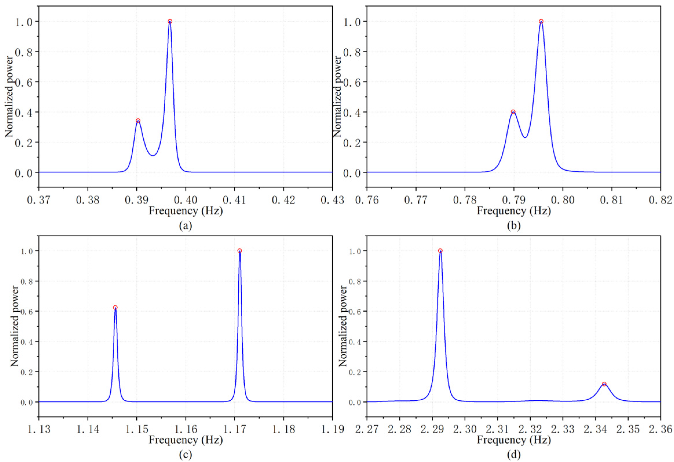
In the original signal, 256 data points were sampled, and the IAA algorithm was used for computation in the small frequency bands partitioned by SFFT. By combining the above results, the results of the SFFT-IAA algorithm were obtained, as shown in Figure 6.

According to Figure 6, in the case of SNR = 30, when the proposed method was used to estimate each harmonic frequency component in each frequency band, the method showed high resolution for frequency estimation, and it was not influenced by other frequency components, with sharp frequency spectra peaks, no frequency aliasing, and strong side lobe suppression. Meanwhile, it distinguished the frequency components that were close to each other.

Similarly, in the case of SNR = 10, the results obtained by the SFFT-IAA algorithm are presented in Figure 7. It can be seen that SNR was 10, influenced by noise, and the side lobe suppression capability was reduced. Although the frequency spectra peaks were not as sharp as those in the case of SNR = 30, the algorithm can still distinguish the frequency components that were close to each other, and the frequency estimation resolution was also high.

To compare the performance of the SFFT-IAA algorithm and the FFT algorithm, simulations using FFT were conducted at an SNR of 10 and 30, respectively. Figure 8 shows the amplitude and frequency characteristics of the eccentricity signal at an SNR of 30 and 10 using FFT.

It can be seen from the Figure 8 that the FFT method showed frequency aliasing around 0.39 Hz, 0.79 Hz, and 1.15 Hz for both SNRs, with low resolution, frequency leakage, and fence effect. Particularly, when SNR was 10, some interference components with frequencies of 0.34 Hz, 0.66 Hz, 1.32 Hz, and 1.56 Hz appeared due to noise interference, and the denoising performance was also poor. The detection results of the frequency, amplitude, and phase angle of the eccentricity signal by the SFFT-IAA and FFT algorithms are presented in

Table 1. The simulation results of eccentricity signal detection.

Eccentricity Parameter	Actual Value	SFFT-IAA		FFT
		SNR = 30	SNR = 10	SNR = 30	SNR = 10
frequency 1/Hz	0.3981	0.3981	0.3968	-	-
amplitude 1/mm	0.2	0.1991	0.1912	-	-
phase angle 1/rad	0	0.0000	0.0003	-	-
frequency 2/Hz	0.3915	0.3915	0.3903	0.3906	0.3906
amplitude 2/mm	0.25	0.2501	0.2417	0.2467	0.2467
phase angle 2/rad	1.5	1.4995	1.4754	1.4758	1.4758
frequency 3/Hz	1.1709	1.1709	1.1710	0.1718	0.1718
amplitude 3/mm	0.15	0.1501	0.1513	0.1737	0.1737
phase angle 3/rad	0.7	0.6998	0.7009	0.7591	0.7591
frequency 4/Hz	1.1456	1.1456	1.1456	-	-
amplitude 4/mm	0.12	0.1200	0.1207	-	-
phase angle 4/rad	0.3	0.3001	0.3003	-	-
frequency 5/Hz	0.7962	0.7962	0.7956	0.8056	0.8056
amplitude 5/mm	0.06	0.0601	0.0058	0.0704	0.0704
phase angle 5/rad	0.8	0.8004	0.7886	0.8943	0.8943
frequency 6/Hz	0.7883	0.7884	0.7898	-	-
amplitude 6/mm	0.03	0.0301	0.0313	-	-
phase angle 6/rad	1.1	1.1008	1.1014	-	-
frequency 7/Hz	2.3417	2.3417	2.3426	2.3438	2.3437
amplitude 7/mm	0.08	0.0800	0.0797	0.0891	0.0891
phase angle 7/rad	1.6	1.6001	1.6013	1.6111	1.6111
frequency 8/Hz	2.2917	2.2917	2.2925	2.2949	2.2949
amplitude 8/mm	0.22	0.2199	0.2230	0.2384	0.2384
phase angle 8/rad	0.2	0.2005	0.2007	0.2295	0.2295

.

The analysis of the data in Table 1 indicated that compared with FFT, SFFT-IAA can obtain more accurate parameters of each harmonic component of the eccentricity signal at different SNRs, thus helping to build a more accurate roll eccentricity signal model. In contrast, the harmonic parameters obtained by the FFT algorithm deviated significantly from the original signal and the accuracy was poor.

According to the above simulation results, under the same noise condition, the proposed SFFT-IAA algorithm achieves significantly higher accuracy for frequency estimation than the FFT algorithm and high frequency resolution in the case of close frequencies. Moreover, with the SFFT-IAA algorithm, the required frequency points can be obtained clearly without band overlapping and the algorithm can overcome the disadvantages of frequency spectral leakage and fence effect of the FFT algorithm, thus showing better overall performance than the FFT algorithm. With a high computational speed and high resolution, the SFFT-IAA algorithm can be applied to reconstruct a more accurate roll eccentricity signal model and can well meet the requirements of roll eccentricity signal detection.

5. Engineering Implementation and Validation

This study conducted engineering application research and algorithm validation of eccentricity compensation by taking an actual 1150 mm six-roller reversible rolling mill as the experimental object. The roller system parameters of the experimental rolling mill are as follows: the upper and lower backup roller diameters are 1018.8 mm and 1052 mm, respectively; the upper and lower intermediate roller diameters are 392.2 mm and 396.36 mm, respectively; the upper and lower work roller diameters are 324.25 mm and 325.72 mm, respectively. The sampling period is 10 ms, and the parameters of the SFFT-IAA algorithm are the same as those used in the simulation.

Roll eccentricity detection and compensation were implemented in the rolling mill AGC system. Considering that the construction algorithm of eccentricity signal detection and eccentricity model based on the SFFT-IAA algorithm is complex and cannot be easily implemented only by the basic automation level (L1), the thickness control system adopts a two-level computer control system combining the basic automation level (L1) and the process automation level (L2). The L2 system adopts industrial control computers to receive and store on-site data and to analyze and to calculate the roll eccentricity signal with advanced language programming. Then, the eccentricity model is constructed and sent to the L1 control system. The L1 control system uses a hardware platform based on Siemens S7-400PLC and Siemens FM458 to receive the eccentricity model and to perform eccentricity compensation control based on the eccentricity model. The 1150 mm six-roller reversible cold rolling mill, rollers, and control system are presented in Figure 9.

The data used to detect the roll eccentricity signals were obtained from the rolling force and outlet thickness deviation data collected on site. The specific steps include:

• Conducting a zero-pressure dependence experiment in the roller gap control mode after each roller change;
• Collecting the rolling force data when the rolling pressure is in the open-loop state;
• Using the collected data to generate the roll eccentricity model.

At this point, without the influence of the rolled piece, the rolling force can fully reflect the roller state and an accurate roll eccentricity model can be established. In the normal rolling process, due to changes in the working condition, the eccentricity model parameters will also change. Therefore, during the rolling process, the thickness fluctuation data of exporting strip steels were collected and then used for online roll eccentricity detection, and the amplitude and the initial phase angle of each harmonic in the eccentricity model established in the zero-pressure dependence state were corrected. Figure 10a shows the rolling force data collected on site at a rolling speed of 1.07036 m/s under the zero-pressure dependence condition. The pressure fluctuation data were divided by the rolling mill stiffness after removing the direct current component and trend processing to obtain the data of the roll gap fluctuation caused by roll eccentricity; the result is shown in Figure 10b.

The L2 computer used the proposed SFFT-IAA to process the collected roll gap fluctuation data. First, SFFT was used to obtain the frequency distribution of the roll eccentricity signal (see Figure 11).

It can be seen from Figure 11 that the frequency components of the measured data were concentrated around 0.33 Hz, 0.63 Hz, 1.73 Hz, and 2.1 Hz, especially around 0.33 Hz, where the component with the largest frequency spectra peak was located. Considering this, four small frequency ranges were set in this study, which were [0.30 Hz 0.36 Hz], [0.60 Hz 0.66 Hz], [1.70 Hz 1.76 Hz], and [2.07 Hz 2.13 Hz]. In each frequency band, the roll eccentricity parameters were estimated by the IAA algorithm; the results are illustrated in Figure 12.

As shown in Figure 12, in the range of [0.30 Hz 0.36 Hz], two frequency components were found, i.e., 0.3244 Hz and 0.3343 Hz; in the range of [0.60 Hz 0.66 Hz], one frequency component was found, i.e., 0.6406 Hz; in the range of [1.70 Hz 1.76 Hz], one frequency component was found, i.e., 1.7371 Hz; in the range of [2.07 Hz 2.13 Hz], two frequency components were found, i.e., 2.102 Hz and 2.092 Hz. Usually, the measured data in the industrial field contain strong noise. According to Figure 11 and Figure 12, the proposed method could effectively eliminate the influence of noise to find the accurate frequency components of the roll eccentricity signal, thus showing a strong interference suppression ability. The results of the eccentricity signal parameters extracted by the proposed method are presented in

Table 2. The experimental results of eccentricity signal detection.

Parameter	1	2	3	4	5	6
frequency/Hz	0.3244	0.3343	0.6406	1.7371	2.0960	2.1003
amplitude/mm	0.0208	0.0220	0.0080	0.0112	0.0051	0.0055
phase angle/rad	0.3504	1.5200	0.7501	1.3301	0.4300	1.5003

.

Moreover, to compare the performance of the SFFT-IAA and the FFT in an engineering application, the experiment using the FFT method was carried out. Figure 13 shows the amplitude and frequency characteristics of the practical eccentricity signal using FFT.

It can be seen from Figure 13 that the FFT method only found four frequencies of 0.3418 Hz, 0.6348 Hz, 1.7333 Hz, and 2.0996 Hz, and no similar frequencies were found. It showed frequency aliasing around 0.34 Hz and 2.09 Hz, with low resolution, frequency leakage, and fence effect. From this experiment, it can be seen that the performance shown by the FFT has no advantage over the SFFT-IAA.

According to the setting of the rolling mill parameters and the production parameters, the roll eccentricity signal comprises the 1× rotation frequencies of two backup rollers, the 2× rotation frequency of a lower backup roller, the 1x rotation frequency of an upper intermediate roller, and the 2× rotation frequencies of two work rollers. This means that the upper backup roller has rotational eccentricity; the lower backup roller has both rotational eccentricity and elliptical eccentricity; the upper intermediate has rotational eccentricity; the two work rolls have elliptical eccentricity. It can be seen that the proposed method is not only meaningful for the accurate detection and compensation control of the eccentricity signal but also for guiding the repair of the rollers.

After the parameters of the eccentricity signal were obtained, the roll eccentricity signal could be reconstructed to establish the eccentricity control and the compensation model. The eccentricity control and the compensation model were constructed by sampling the eccentricity signal of the roller with the largest diameter at $M$ equal intervals after one cycle of rotation, and a sequence $E$ can be obtained as:

$$E^T=\left[e\left(1\right),\cdots , e\left(M\right)\right]$$

(26)

Figure 14 illustrates the eccentricity control model at $M=128$.

Then, the roll eccentricity model $E$ was sent from the L2 computer to the L1 controller, and in the L1 controller, the eccentricity model was reversely compensated to the roll gap control loop. In the experiment, the eccentricity compensation control was put in the first pass of rolling. The thickness deviation of the exporting strip steels before and after the eccentricity compensation control is shown in Figure 15.

After the eccentricity compensation control was performed, the thickness deviation of the exporting strip steels was reduced by 89.2%, indicating good compensation effects. The experimental results indicated that the proposed method can be used to establish a highly accurate eccentricity model and can meet the requirements of engineering applications.

6. Conclusions

This study focused on roll eccentricity signal detection and eccentricity compensation, which is key to improving the quality of finished strip steels. In this study, a roll eccentricity signal detection method was proposed based on SFFT-IAA, and the applications of the proposed method and the roll eccentricity compensation and control in practical engineering were investigated through experiments. The method proposed has not been reported in the field of roll eccentricity compensation, especially focusing on estimating similar frequency components in the eccentricity signal. The innovation of the proposed method is to improve the IAA, which makes full use of the rapidity of SFFT and the accuracy of the IAA algorithm; the accuracy and speed of the roll eccentricity signal detection are improved significantly. The proposed method has no particularly complicated calculation steps. It is easy to be implemented by computer programs and suitable for engineering applications. In the simulation experiments, the proposed method can find all eight frequencies of the simulated signal, and the average accuracy of the proposed method is 99.99% and 99.88% when SNR = 30 and SNR = 10, respectively. When this method was applied in engineering experiments, the thickness fluctuation of exporting strip steels was reduced by 89.2% and the product quality was significantly improved, indicating a high application value in engineering applications. Simulation and practical engineering experiments revealed that the proposed method has a fast computational speed and a strong anti-interference ability and it can distinguish the harmonic components with very similar frequencies in the roll eccentricity signal, thus the proposed method can be used to establish a highly accurate roll eccentricity model. In the study, limitations of the proposed method were also found. As the SNR decreases, the accuracy of the IAA step of the proposed method decreases significantly and satisfactory results cannot be obtained. Subsequent work will further investigate to improve the anti-noise performance of the proposed method. At the same time, the proposed method has many calculation steps, and the proposed algorithm has many calculation steps; therefore, reducing the complexity of the algorithm is also the content of further research.