Article

Adjustable Capacity Evaluation Method Based on Step-by-Step Power Mapping of Offshore Wind Farms

1
NARI Technology Co., Ltd., Nanjing 211106, China
2
College of Energy and Electrical Engineering, Hohai University, Nanjing 211100, China
3
State Grid Suzhou Power Supply Company, Suzhou 215000, China
4
School of Electrical Engineering, Southeast University, Nanjing 210096, China
*
Author to whom correspondence should be addressed.
Appl. Sci. 2022, 12(17), 8644; https://doi.org/10.3390/app12178644
Submission received: 11 July 2022 / Revised: 18 August 2022 / Accepted: 22 August 2022 / Published: 29 August 2022
(This article belongs to the Special Issue State-of-the-Art of Power Systems)

Abstract

:
Offshore wind power has developed rapidly in recent years, but its scale still lags far behind onshore wind power. Offshore wind power still has great development potential. One of the key factors restricting the development of offshore wind power is the unsatisfactory control effect of offshore wind farms, and the reason is that the adjustable capacity of the wind farm cannot be obtained accurately and quickly. Aims to meet the high precision requirements for adjustable capacity evaluation of offshore wind farms, this paper establishes a step-by-step power mapping framework based on the division of power transmission processes in offshore wind farms, considering the loss of each transmission process in detail. By establishing a step-by-step mapping from the wind turbine power to the injected power at the grid connection point of the offshore wind farm, the adjustable capacity of the offshore wind farm can be estimated based on the maximum theoretical power of the wind turbines. The performance of proposed method has been demonstrated in a real offshore wind farm.

1. Introduction

Building the power system with renewable energy as the main energy source is the important measure to reduce carbon emissions. The development cost of wind energy is lower than that of solar energy, and the safety of wind power generation is better than that of nuclear power generation. In view of the advantages of wind energy in the field of clean energy, wind power has developed rapidly in recent years, especially offshore wind power. In 2021, China’s new installed capacity of offshore wind power reaches 1.8 times the previous cumulative installed capacity. Despite this, onshore wind power still occupies more than 90% of the share, and offshore wind power still has huge development potential.
The application of long-distance offshore transmission lines, power electronics, and large transformers has caused significant power quality problems and challenges in voltage and frequency stability to the grids connected to offshore wind farms [1,2,3,4].
To overcome the power quality problem, the combination of high-frequency switchgear and reactive power compensation equipment can change the parameters of the grid to alleviate the problem [5]. The establishment of combined power plants can reduce the impact of power changes on the grid and promote the consumption of renewable energy. The comprehensive utilization of offshore wind energy and wave energy to establish a combined power plant can reduce short-term power changes, which is conducive to the integration of the power plant into the grid [6]. Reference [7] proposed a system for incorporating multiple distributed offshore wind farms into an onshore grid. A system control strategy was established for the circulating current converter. At the same time, a new black-start method and a comprehensive primary frequency control scheme were designed. Reference [8] designed a DC transmission system for offshore wind farms, and applied a new modular multi-channel DC converter. The control strategy of the grid-connected scheme can maintain the current-voltage balance of the DC transformer while achieving maximum power control. Reference [9] proposed a coordinated control strategy that can provide inertia support for the power grid, which realized cascade control by means of the communication between the offshore power grid and the onshore power grid. References [10,11,12,13,14,15] analyzed the reliability and economy of off grid hybrid energy system using wind power, and pointed out that this system is an effective solution to solve the energy supply in remote areas.
There are some other studies on grid-connected system construction and control strategy establishment for offshore wind farms [16,17,18,19,20,21]. At present, most of the researches on grid connection of offshore wind farms focus on these two aspects, and the estimation of adjustable capacity is rarely mentioned. The offshore wind farm has two independent monitoring systems. One is the SCADA (Supervisory Control And Data Acquisition) system of the wind turbine, and the other is the monitoring system responsible for collecting other data. The wind farm inputs the collected data into the AGC (Automatic Generation Control) system for analysis and calculation, and then reports the calculated adjustable capacity to the dispatching department of power grid. The dispatching department of power grid issues orders to offshore wind farms according to the adjustable capacity. Therefore, the accuracy of the adjustable capacity calculation affects the control effect. The method currently used in offshore wind farms is to directly multiply the power of the wind turbine by the empirical coefficient to obtain the adjustable capacity, which has a large error.
Since the wind turbine is far from the land, various losses will be generated when transmitting electricity. When calculating the loss, the physical model requires too many parameters, and the calculation process is complicated. Moreover, the marine environment is changeable, so the parameters measured by experiments are not accurate. This leads to a large error in calculating the grid-connected adjustable capacity of offshore wind farms using the maximum theoretical power of wind turbines. It is difficult to accurately control and dispatch wind farms, which will further affect the consumption of offshore wind power. Compared with the physical model, the data-driven model is more rapid and simple, and the accuracy of the calculation results is higher. The adjustable capacity can be calculated by inputting the power of the wind turbine.
In order to improve the calculation accuracy of the adjustable capacity of offshore wind farms, this paper establishes power mappings for each power transmission process in offshore wind farms. The losses of each process is analyzed and modeled separately, and the step-by-step mapping from the power of the wind turbines to the power of the grid connection point of the wind farm is realized. Firstly, spectral clustering is used to classify wind turbines to reduce the dimension of input data and reduce the difficulty of model fitting. Then, the neural network is used to calculate the power of the collector system and the loss of the submarine cable. Finally, other losses of the offshore wind farm are statistically analyzed and the adjustable capacity is calculated. In this way, the adjustable capacity of wind farm can be evaluated based on the maximum theoretical generating power of wind turbines.

2. Division of Power Transmission Links in Offshore Wind Farms

The power of the offshore wind farm is generated by the wind turbines. After collecting electricity and boosting, it is transmitted to the onshore part through a long-distance high-voltage submarine cable for grid connection. During the transmission process, losses will occur in various processes. Therefore, the adjustable capacity reported by the AGC system of the wind farm to the power grid dispatching department needs to be corrected on the basis of the maximum theoretical power of the wind turbine. However, the current calculation method of the adjustable capacity used by wind farms is not accurate enough to meet the requirements of the power grid. This paper will sort out the power transmission processes of offshore wind farms, and establish a power map of wind farms considering the losses in each transmission process, so as to estimate the adjustable capacity of offshore wind farms based on the maximum theoretical generating power of wind turbines.
The offshore wind farm can be divided into two parts: offshore part and onshore part. The connection between these two parts is realized by transmitting power through high-voltage submarine cables. Figure 1 shows the basic structure of a typical offshore wind farm.
The collector system collects and boosts the power generated by wind turbines, and then transmits it to the onshore part through the high-voltage submarine cable. After deducting the loss of onshore part, the power delivered to the land that finally flows into the grid is the grid-connected power of the wind farm. The power of the grid connection point corresponds to the real-time power of the wind turbine, while the adjustable capacity of the wind farm corresponds to the maximum theoretical power of the wind turbine. To achieve adjustable capacity evaluation, it is necessary to first establish a mapping between the power of wind turbines and the power of the grid connection point.
Based on the offshore wind farm structure shown in Figure 1, the power transmission of the wind farm can be divided into three main processes:
(1)
Power transmission from wind turbines to the head of the high-voltage submarine cable. This process includes power collection and boosting. The power loss includes the loss generated by the collector system and the station power in the offshore part.
(2)
High-voltage submarine cable transmission section. In this process, the submarine cable transmits power from the offshore to the onshore part. The main reason for power loss is that during the power transmission process, each component of the submarine cable will generate power loss due to the rise in temperature and the establishment of electric and magnetic fields.
(3)
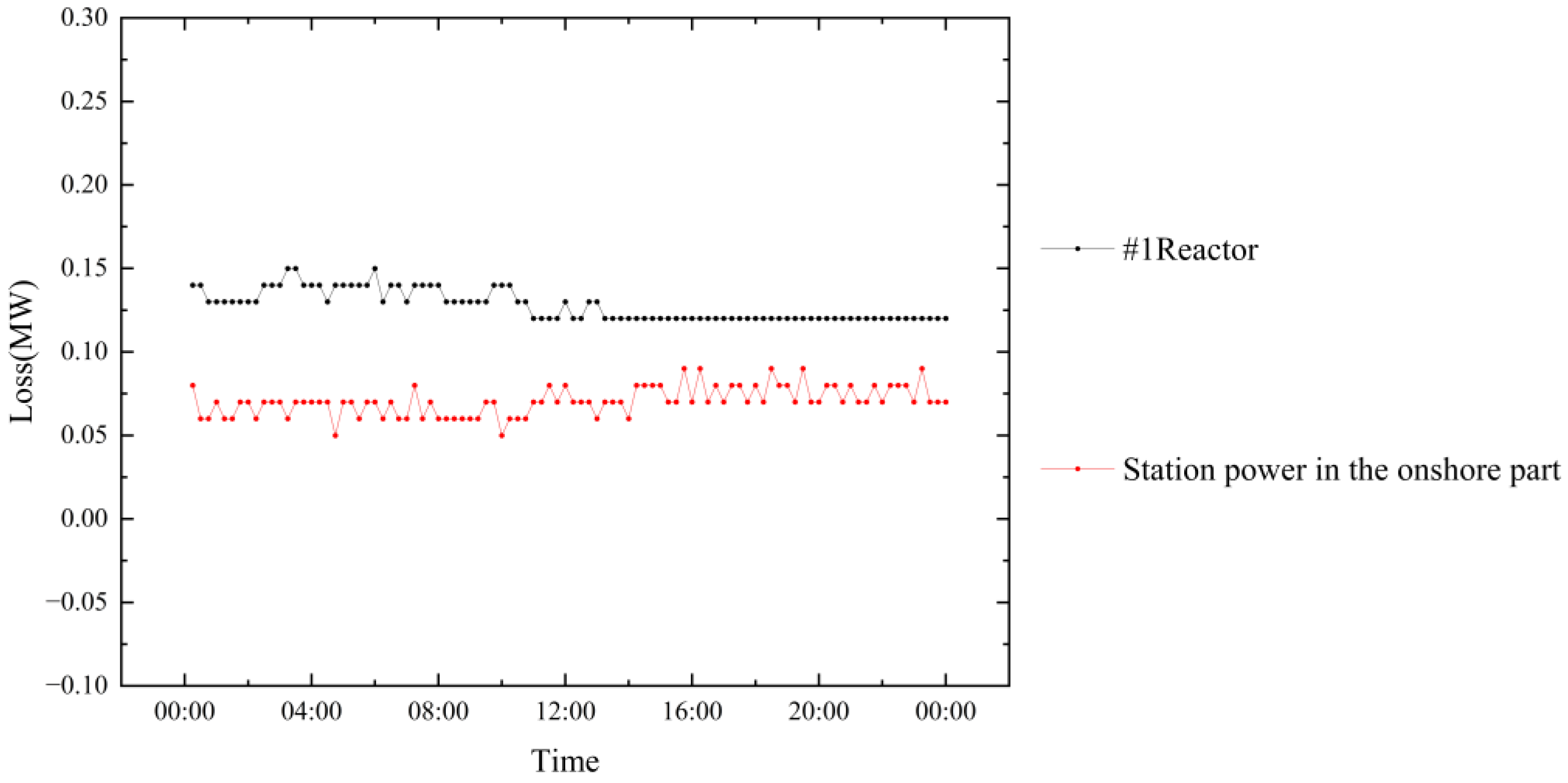
Power transmission from the end of the high-voltage submarine cable to the grid connection point. In this process, the power is transmitted to the onshore part of the wind farm and then fed into the power grid. The power loss comes from the station power in the onshore part and the consumption of other compensation equipment.

3. Step-by-Step Mapping of Offshore Wind Farm Power

According to the higher precision requirements of offshore wind farms for adjustable capacity, this paper considers the loss of each transmission process in detail, and establishes a step-by-step mapping of the power of offshore wind farms. Based on the division of power transmission processes, the power mapping is divided into three sections. The first section is from the wind turbine to the power collector system, and the BP network is used to realize the mapping between the two powers. The second section is the power mapping between the power collector system to the end of the submarine cable power, and this part of the loss is mainly generated by the high-voltage submarine cable. The BP network is used to calculate the cable loss. The third section is the part from the end of the submarine cable to the grid connection point, and the power consumption model of the onshore station power consumption and compensation equipment is established. By establishing the step-by-step mapping from wind turbine power to grid connection point power of offshore wind farms, it is possible to estimate the adjustable capacity based on the maximum theoretical power of wind turbines.

3.1. Mapping of Wind Turbine Power to Collector System Power

There are two ways to calculate the cable loss: using the wind turbine power to directly calculate the cable loss or mapping the wind turbine power to an intermediate variable to calculate the line loss. According to the division of the power transmission process of the wind farm, the power of the collector system is selected as the intermediate variable. Figure 2 shows the power collector system of the offshore wind farm.
The power emitted by the wind turbine is raised from low voltage to medium voltage by the transformer and then merged into the bus bar through the collector line. In this process power loss will occur, so the sum of the distributed fan power cannot be directly used as the power of the collector system. Otherwise, there will be a large error when calculating the cable loss.
Based on the BP (Back Propagation) neural network, this paper establishes the connection between the power of the wind turbines and the power of the collector system. The structure of BP neural network is shown in Figure 3.
In the above figure, the input vector is X = ( x 1 , x 2 , , x n ) T , the output of the hidden layer is Y = ( y 1 , y 2 , , y m ) T , the output of the output layer is O = ( o 1 , o 2 , o l ) T . ω i j is the connection weight from the input layer to the hidden layer. ω j k is the connection weight from the hidden layer to the output layer.
The mathematical model of the BP neural network is as follows
y j = f ( i = 1 n ω i j x i ) j = 1 , 2 , m
o k = f ( j = 1 m ω j k y j ) k = 1 , 2 , l
where f ( · ) is the activation function of the network. The formula for determining the number of neurons in the hidden layer is as follows
m < ( n + l ) + a ,
where m is the number of hidden layer nodes, n is the number of input layer nodes, l is the number of output layer nodes, a is a constant between 0 and 10. Training is performed by setting different numbers of hidden layer nodes, and finally the model with the smallest error is selected.
Considering the large number of wind turbines in offshore wind farms, direct fitting may not be effective. Therefore, spectral clustering of wind turbines is performed to reduce the data dimension of the input data.
Assuming that the number of wind turbines is a , and each unit has historical power data of b time points, then the power sequence of the wind farm can be written as the following matrix.
X = [ x 1 , x 2 , , x a ] T = [ x 11 x 1 b x a 1 x a b ] a × b ,
where x 1 , x 2 , , x a is the row vector formed by the historical power sequence of each wind turbine, and the dimension is b .
To quantify the similarity of the power data, set the vector Q = [ q 1 , q 2 , , q n ] , O = [ o 1 , o 2 , , o n ] . The Pearson correlation coefficient can be calculated as
p Q O = i = 1 n ( q i q ¯ ) ( o i o ¯ ) i = 1 n ( q i q ¯ ) 2 i = 1 n ( o i o ¯ ) 2 ,
where q ¯ is the average value of Q , o ¯ is the average value of O .
The specific steps of spectral clustering are as follows:
(1)
For the power sequence vector of any wind turbine i and wind turbine j in the offshore wind farm, calculate the Pearson coefficient between the two and denote it as p i j , and then construct the similarity matrix P :
P = [ p 11 p 1 a p a 1 p a a ] a × a ,
(2)
Based on the similarity matrix P , calculate the degree matrix H
H = [ h 1 0 0 0 h 2 0 0 0 h a ] a × a ,
where h i is the sum of the elements in the i-th row of matrix P , and the matrix H is a diagonal matrix.
(3)
Construct the Laplacian matrix L , and normalize it.
L = H P ,
L = H 0.5 L H 0.5 ,
(4)
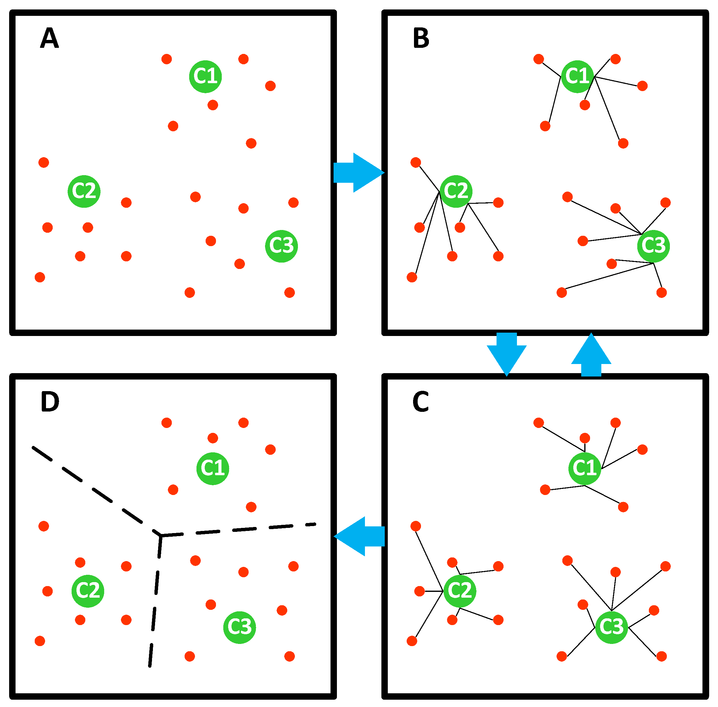
Determine the number of spectral clusters k . Calculate the first k minimum eigenvalues of L and the corresponding eigenvectors, and normalize the eigenvectors to construct a new matrix U a × k .
(5)
K-means clustering is performed on the row vector of the matrix U a × k . Based on the distance between the calculated sample and the center point, the samples belonging to each cluster are summarized, and iteratively realizes the minimum distance between the sample and the center of the cluster to which it belongs.
Firstly, k samples are randomly selected as the initial cluster centers.
Secondly, for each sample, calculate its Euclidean distance to k cluster centers. And assign it to the cluster corresponding to the cluster center with the smallest distance.
Then, for each cluster, recalculate its cluster center position.
Finally, repeat the above two steps until the number of iterations reaches the upper limit or the position of the cluster center remains unchanged.
The clustering process is shown in Figure 4, C1, C2 and C3 are cluster centers.
The division of k clusters of wind turbines C 1 , C 2 , , C k is obtained to realize the spectral clustering of wind turbines.
Based on the clustering results of wind turbines, calculate the matrix Z of the total power of wind turbines in k clusters
Z = [ z 11 z 1 b z k 1 z k b ] k × b ,
where, the ith row vector of Z represents the time series of the total wind turbine power in the ith cluster. Different clustering results are obtained by setting different clustering numbers, and finally the one with the smallest error is selected.
Taking the wind turbine clustering power as the input and the collector system power as the output, the mapping can be established based on the BP neural network.
P G = f 1 ( P Z ) ,
where P G is collector system power, P Z is the wind turbine clustering power, f 1 ( · ) is the trained network model.

3.2. Mapping of Collector System Power to Submarine Cable End Power

After getting the power of the collector system, we can use it as the input to calculate the loss of the submarine cable by the BP network.
P C = f 2 ( P G ) ,
where P C is total loss of high voltage submarine cable, f 2 ( · ) is the trained network model.
The power of the collector system connects the first and second sections of the offshore wind farm power step-by-step mapping model. It plays an important role in the calculation of the cable loss. It is the key variable of the model. The power of the collector system minus the line loss of the wind farm offshore station and the submarine cable is the power at the end of the submarine cable. The process is shown in Figure 5.

3.3. The Mapping from the Power at the End of the Submarine Cable to the Power at the Grid Connection Point

Figure 6 shows the structure of the onshore part of the offshore wind farm.
The power at the end of the submarine cable is first collected into the bus, and a part of the power is reduced for electric field consumption, including reactive power compensation equipment, reactors, and station electricity. By analyzing and calculating the characteristics of various losses respectively, the power at the end of the submarine cable minus all losses is the power at the grid connection point
P K = s u m ( P G ) P C P t P s ,
where P K is the grid connection point power, s u m ( · ) is vector summation, P t is station power, P s is the loss of compensation equipment. If the maximum theoretical generated power of the wind turbine is input when calculating the power of the collector system, the final calculation result is the adjustable capacity of the offshore wind farm.

4. Result

The data used in the calculation example comes from an offshore wind farm in Jiangsu, with a total of 67 wind turbines. All wind turbines are distributed on 12 collector lines, and the electric energy is first collected by the collector system, then boosted, and transmitted to the onshore part of the wind farm through high-voltage submarine cables for grid connection. The data of the wind farm was collected for 9 days, and the time interval was 15 min. The data of the first 8 days was used for training, and the data of the last day was verified.

4.1. Analysis and Calculation of Submarine Cable Loss

The power curve of the wind farm is shown in Figure 7.
As can be seen from the figure, before about 14:00, the power of the wind farm was maintained at a high level, and the total power was greater than 150 MW. After 14:00, the total power of the wind farm dropped significantly, and the overall power was lower than 100 MW. Moment power is close to zero.
The loss of the wind farm is shown in Figure 8.
Combined with Figure 7, it can be found that the submarine cable loss has a strong positive correlation with the power, so the power is selected as the input of the neural network. The evaluation index of the calculation results adopts the Mean Absolute Error ( M A E ) and the Root Mean Square Error ( R M S E ).
M A E = 1 N i = 1 N | y ^ i y i | ,
R M S E = 1 N i = 1 N ( y ^ i y i ) 2 ,
where N is the number of samples, y ^ i is calculated value, y i is actual value.
Figure 9 shows the result of calculating the loss of the submarine cable using the wind turbine power, the number of hidden layer nodes is set to 8. Figure 10 shows the result of using the collector system, the number of hidden layer nodes is set to 5. The error comparison is shown in Table 1.
From the comparison of the calculation results and errors, it can be seen that the calculation using the power of the collector system can better reflect the real change trend of the submarine cable loss, and the error is significantly lower than that of the wind turbine power. This is because the dimension of the fan power data is high, which affects the fitting effect. The dimension of the data is reduced after using the power of the collector system, so the error is smaller.

4.2. Other Losses

In addition to the loss of submarine cables, the losses of offshore wind farms also include power consumption of substations and compensation equipment losses. The onshore losses in Figure 8 include the station power consumption and compensation equipment losses in the onshore part. Combining with Figure 7, it can be seen that the onshore losses are negatively correlated with the transmission power. The active power loss of the static var generator (SVG) is shown in Figure 11, and the power consumption of the reactor and the electricity used by the onshore station is shown in Figure 12.
Combined with the power curve of the wind farm in Figure 7, it can be seen that the power consumption of the static var generator is obviously negatively correlated with the transmission power. When the transmission power of the wind farm is high, the power consumption of the static var generator is basically 0, and the transmission power is low. At a certain value, the power consumption of the static var generator will basically remain a fixed value. However, the power consumption of reactors and onshore stations has no obvious relationship with the transmission power of the wind farm, and always remains at a certain level with a small fluctuation range. Therefore, it can be judged that the main reason for the change in the loss of the onshore part of the wind farm is that the power consumed by the static var generator changes with the fluctuation of the transmission power of the wind farm.
In addition, it can be seen from Figure 8 that the station loss in the offshore part varies little and is always maintained within a certain range. Several losses except submarine cable losses have certain regularity, so they are statistically modeled by analyzing data. The station loss of the offshore part of the wind farm is taken as 0.5 MW, the station loss of the onshore part is taken as 0.07 MW, and the reactor loss is taken as 0.13 MW. The losses of the static var generator are as follows
P S V G # 1 = { 0.33 , P 220 < 130 0 , P 220 > 130 ,
P S V G # 2 = { 0.24 , P 220 < 130 0 , P 220 > 130 ,
where P S V G # 1 and P S V G # 2 are losses of SVG, P 220 is the power injected into the onshore 220 kV busbar.

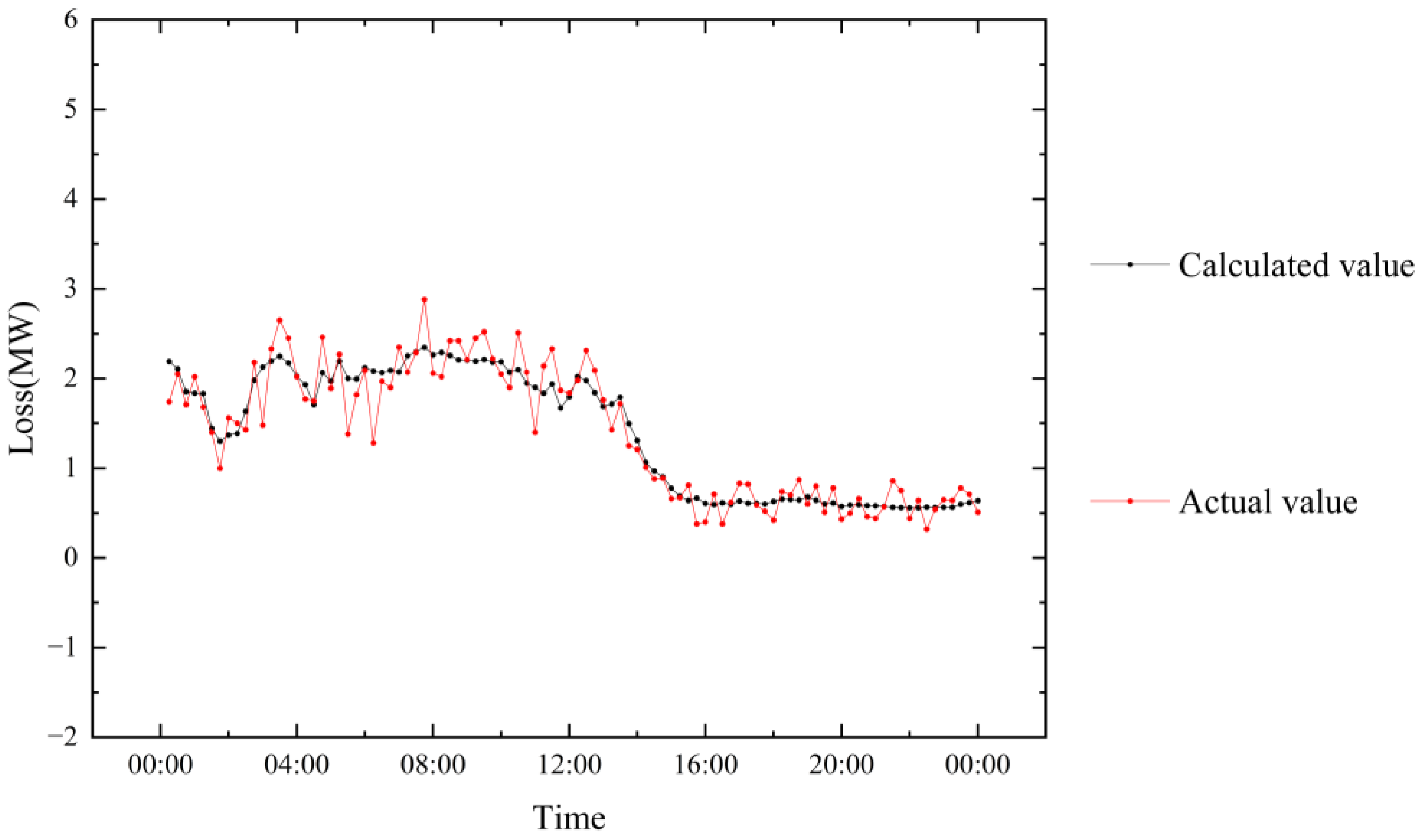
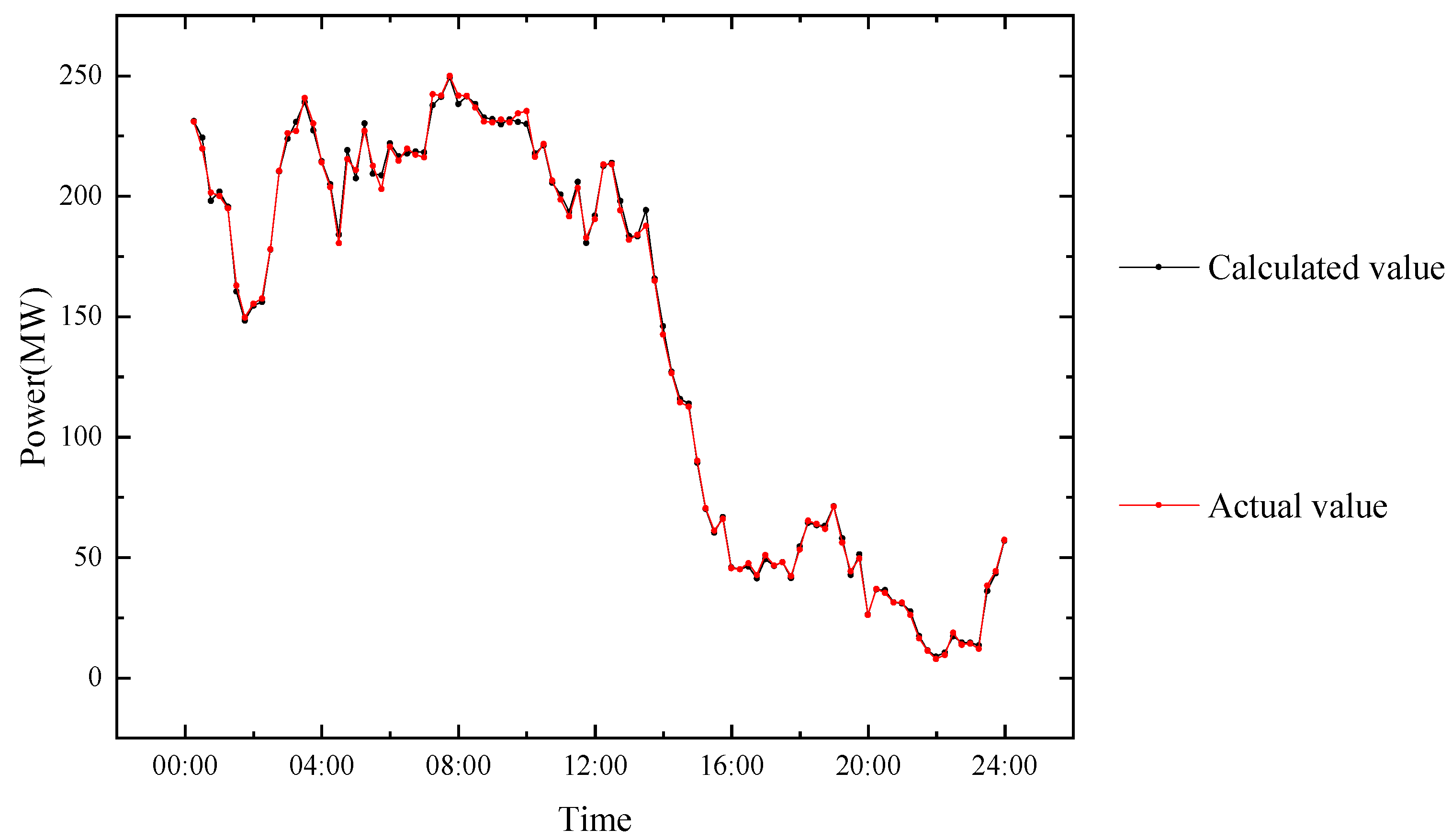
4.3. Wind Farm Power Mapping

Input the clustered power of the wind turbines into the first mapping to calculate the power of the collector system. The number of clusters is 12, and the number of hidden layer nodes of the neural network is set to 8. The results are shown in Figure 13.
Comparing the errors calculated by the clustered power and the original power of the wind turbines, the errors are shown in Table 2.
It can be seen from the error comparison that the error of the collector system power calculating after the wind turbine power is spectrally clustered is smaller than that of using the original power.
The calculated power of the collector system is input into the BP network to calculate the submarine cable loss, and the results are shown in Figure 14.
The M A E is 0.18 MW and R M S E is 0.24 MW, which is almost the same as the error in the first part of the example analysis, indicating that the power fitting effect of the power collection system is ideal.
After the calculation results of the collector system power and the cable loss of the submarine cable are obtained, the power of the collector system is subtracted from the loss of the offshore station, the loss of the submarine cable, and the loss of the onshore part at the corresponding time point, which is the final power of the grid connection point. The calculation results are shown in Figure 15.
In the practical application of offshore wind farms, the SCADA system of the wind turbine is independent of the monitoring systems of other parts, and only collects the relevant data of the wind turbines, and the wind farm AGC system uses the collected maximum theoretical power of the wind turbine to convert the wind farm’s possible output. In order to verify the effectiveness of the method proposed in this paper, the two methods are compared:
Method 1: In the segmented power mapping model proposed in this paper, the wind turbine power is input into the wind turbine power to collector system power mapping, and then the collector system power mapping result is input into the submarine cable loss calculation model. The power of the collector system after deducting various losses is the power at the grid connection point of the wind farm.
Method 2: Direct power mapping model, which takes the power of each wind turbine as the input and the power of the wind farm grid connection point as the output, and calculates based on the BP network.
The errors calculated by the two methods are compared in Table 3.
By comparison, it can be seen that the step-by-step mapping method of wind farm power proposed in this paper can better reflect the real change trend than the direct calculation of wind turbine power. And the error is significantly reduced, which verifies the effectiveness and superiority of the proposed method.
Compared with the direct mapping method, the loss in the power transmission process of the wind farm is considered more carefully. The calculation of the cable loss of the submarine cable is taken into account, and the power model of plant power and reactive power devices is realized. The characteristic modeling of the model effectively reduces the calculation error. Using the maximum theoretical generating power of wind turbines to calculate based on the method proposed in this paper, the adjustable capacity of offshore wind farms can be obtained, which provides a reference for grid dispatching.

5. Conclusions

The power generated by the wind turbines in the offshore wind farm generates various losses during the transmission to the onshore grid connection point. Therefore, it needs to be corrected based on the maximum theoretical power of the wind turbine and then reported as an adjustable capacity. The cable loss and other losses are used to realize the step-by-step mapping of the wind farm power, and a mapping model is established based on the actual offshore wind farm.
Based on the wind farm power step-by-step mapping model, an adjustable capacity estimation method is established. In practical applications, the adjustable capacity of the offshore wind farm can be obtained by taking the real-time maximum theoretical power of each wind turbine provided by the wind turbine SCADA system as the input. An example analysis is carried out using the actual data of offshore wind farms. Compared with the direct power mapping model, the step-by-step mapping method of wind farm power proposed in this paper considers the losses in the power transmission process of the wind farm more efficiently. The calculation result is closer to the actual value, and the error is significantly reduced. The effectiveness and superiority of this method are verified. However, there is still room for further improvement in the calculation effect of submarine cable loss and the modeling of other losses can be more refined, which will be the direction of our future work.

Author Contributions

Conceptualization, X.D.; Data curation, J.Z. (Jingtao Zhao); Formal analysis, J.Z. (Jingtao Zhao), Z.L., J.Z. (Junpeng Zhu) and Z.W.; Investigation, X.D.; Methodology, J.Z. (Jingtao Zhao), Z.L., S.Z. and J.Z. (Junpeng Zhu); Resources, X.D. and S.Z.; Software, S.Z.; Supervision, Z.W.; Writing—original draft, Z.L.; Writing—review & editing, X.D., J.Z. (Junpeng Zhu) and Z.W. All authors have read and agreed to the published version of the manuscript.

Funding

This research received no external funding.

Data Availability Statement

Data is provided by third parties and is not shared.

Conflicts of Interest

The authors declare no conflict of interest.

References

  1. Cai, X.; Yang, R.; Zhou, J.; Fang, Z.; Yang, M.; Shi, X.; Chen, Q. Review on Offshore Wind Power Integration via DC Transmission. Autom. Electr. Power Syst. 2021, 45, 2–22. [Google Scholar]
  2. Zhang, Z.; Shi, W.; Qu, J.; Bai, H. Grid Connection and Transmission Scheme of Large-Scale Offshore Wind Power. Strateg. Study CAE 2021, 23, 182–190. [Google Scholar] [CrossRef]
  3. Chi, Y.; Liang, W.; Zhang, Z.; Li, Y. An Overview on Key Technologies Regarding Power Transmission and Grid Integration of Large Scale Offshore Wind Power. Proc. CSEE 2016, 36, 3758–3771. [Google Scholar]
  4. Yao, W.; Xiong, Y.; Yao, Y.; Li, Y.; Xin, H.; Wen, J. Review of Voltage Source Converter-based High Voltage Direct Current Integrated Offshore Wind Farm on Providing Frequency Support Control. High Volt. Eng. 2021, 47, 3397–3413. [Google Scholar]
  5. Ali, S.W.; Sadiq, M.; Terriche, Y.; Naqvi, S.A.R.; Hoang, L.Q.N.; Mutarraf, M.U.; Hassan, M.A.; Yang, G.; Su, C.-L.; Guerrero, J.M. Offshore Wind Farm-Grid Integration: A Review on Infrastructure, Challenges, and Grid Solutions. IEEE Access 2021, 9, 102811–102827. [Google Scholar] [CrossRef]
  6. Stoutenburg, E.D.; Jacobson, M.Z. Reducing Offshore Transmission Requirements by Combining Offshore Wind and Wave Farms. IEEE J. Ocean. Eng. 2011, 36, 552–561. [Google Scholar] [CrossRef]
  7. Li, C.; Zhan, P.; Wen, J.; Yao, M.; Li, N.; Lee, W.-J. Offshore Wind Farm Integration and Frequency Support Control Utilizing Hybrid Multiterminal HVDC Transmission. IEEE Trans. Ind. Appl. 2014, 50, 2788–2797. [Google Scholar] [CrossRef]
  8. Hu, P.; Yin, R.; He, Z.; Wang, C. A Modular Multiple DC Transformer Based DC Transmission System for PMSG Based Offshore Wind Farm Integration. IEEE Access 2020, 8, 15736–15746. [Google Scholar] [CrossRef]
  9. Li, Y.; Xu, Z.; Ostergaard, J.; Hill, D.J. Coordinated Control Strategies for Offshore Wind Farm Integration via VSC-HVDC for System Frequency Support. IEEE Trans. Energy Convers. 2017, 32, 843–856. [Google Scholar] [CrossRef]
  10. Arefin, S.S. Optimization Techniques of Islanded Hybrid Microgrid System. In Renewable Energy—Resources, Challenges and Applications; Qubeissi, M.A., El-kharouf, A., Soyhan, H.S., Eds.; IntechOpen: London, UK, 2020; Volume 24, pp. 465–482. [Google Scholar]
  11. Shezan, S.A.; Ishraque, M.F. Assessment of a Micro-grid Hybrid Wind-Diesel-Battery Alternative Energy System Applicable for Offshore Islands. In Proceedings of the 2019 5th International Conference on Advances in Electrical Engineering (ICAEE), Dhaka, Bangladesh, 26–28 September 2019. [Google Scholar]
  12. Shezan, S.A.; Saidur, R.; Ullah, K.R.; Hossain, A.; Chong, W.T.; Julai, S. Feasibility analysis of a hybrid off-grid wind–DG-battery energy system for the eco-tourism remote areas. Clean Technol. Environ. Policy 2015, 17, 2417–2430. [Google Scholar] [CrossRef]
  13. Shezan, S.A.; Ali, S.S.; Rahman, Z. Design and implementation of an islanded hybrid microgrid system for a large resort center for Penang Island with the proper application of excess energy. Environ. Prog. Sustain. Energy 2020, 40, e13584. [Google Scholar] [CrossRef]
  14. Shezan, S.; Das, N.; Mahmudul, H. Techno-economic Analysis of a Smart-grid Hybrid Renewable Energy System for Brisbane of Australia. Energy Procedia 2017, 110, 340–345. [Google Scholar] [CrossRef]
  15. Shezan, S.; Ping, H. Techno-Economic and Feasibility Analysis of a Hybrid PV-Wind-Biomass-Diesel Energy System for Sustainable Development at Offshore Areas in Bangladesh. Curr. Altern. Energy 2017, 1, 20–32. [Google Scholar] [CrossRef]
  16. Wu, Y.-K.; Chang, S.-M.; Mandal, P. Grid-Connected Wind Power Plants: A Survey on the Integration Requirements in Modern Grid Codes. IEEE Trans. Ind. Appl. 2019, 55, 5584–5593. [Google Scholar] [CrossRef]
  17. Ji, K.; Tang, G.; Pang, H.; Yang, J. Impedance Modeling and Analysis of MMC-HVDC for Offshore Wind Farm Integration. IEEE Trans. Power Deliv. 2020, 35, 1488–1501. [Google Scholar] [CrossRef]
  18. Komiyama, R.; Fujii, Y. Large-scale integration of offshore wind into the Japanese power grid. Sustain. Sci. 2021, 16, 429–448. [Google Scholar] [CrossRef]
  19. Perveen, R.; Kishor, N.; Mohanty, S.R. Off-shore wind farm development: Present status and challenges. Renew. Sustain. Energy Rev. 2014, 29, 780–792. [Google Scholar] [CrossRef]
  20. Mitra, P.; Zhang, L.; Harnefors, L. Offshore Wind Integration to a Weak Grid by VSC-HVDC Links Using Power-Synchronization Control: A Case Study. IEEE Trans. Power Deliv. 2014, 29, 453–461. [Google Scholar] [CrossRef]
  21. Guo, G.; Song, Q.; Zhao, B.; Rao, H.; Xu, S.; Zhu, Z.; Liu, W. Series-Connected-Based Offshore Wind Farms with Full-Bridge Modular Multilevel Converter as Grid- and Generator-side Converters. IEEE Trans. Ind. Electron. 2020, 67, 2798–2809. [Google Scholar] [CrossRef]
Figure 1. The structure of a typical offshore wind farm.
Applsci 12 08644 g001
Figure 2. Power collector system of the offshore wind farm.
Applsci 12 08644 g002
Figure 3. The structure of BP neural network.
Applsci 12 08644 g003
Figure 4. The process of K-means clustering. (A) The initial cluster centers are randomly selected. (B) Calculate the distance between the sample and the cluster center and classify samples. (C) Reselect cluster centers. (D) The clustering result is confirmed.
Applsci 12 08644 g004
Figure 5. Mapping process from wind turbine power to the power at end of submarine cable.
Applsci 12 08644 g005
Figure 6. The structure of the onshore part of the offshore wind farm.
Applsci 12 08644 g006
Figure 7. Power curve of offshore wind farm.
Applsci 12 08644 g007
Figure 8. The loss of the wind farm.
Applsci 12 08644 g008
Figure 9. Calculation of cable loss results based on wind turbine power.
Applsci 12 08644 g009
Figure 10. Calculation of cable loss results based on the power of the collector system.
Applsci 12 08644 g010
Figure 11. The loss of SVG.
Applsci 12 08644 g011
Figure 12. Power consumption of reactors and onshore stations.
Applsci 12 08644 g012
Figure 13. Calculation results of mapping from wind turbine clustered power to collector system power.
Applsci 12 08644 g013
Figure 14. Result of cable loss calculation.
Applsci 12 08644 g014
Figure 15. Step-by-step mapping of grid connection point power calculation results.
Applsci 12 08644 g015
Table 1. Error comparison of submarine cable loss calculation results.
InputMAE (MW)RMSE (MW)
Wind turbine power0.240.31
Power of the collector system0.180.23
Table 2. Comparison of errors in the power calculation results of the collector system.
InputMAE (MW)RMSE (MW)
Original power1.962.75
Clustered power1.632.14
Table 3. Error comparison of grid connection power calculation results.
MAE (MW)RMSE (MW)
Segmented Mapping Model1.592.08
Direct Mapping Model2.553.73
Publisher’s Note: MDPI stays neutral with regard to jurisdictional claims in published maps and institutional affiliations.

