1. Introduction
The retail sector dominates a big proportion of the service industry in modern countries because it provides a variety of the goods necessary for daily consumption [
1,
2]. Generally, retail chains consist of four specific systems: department stores, hypermarkets, supermarkets, and convenience stores. Specifically, households are the primary customers for hypermarkets and supermarkets, while individuals are the primary customers for department stores and convenience stores. Clearly, the product categories, geographical locations, area sizes, and make-up of the main customers are quite different between portions of the retail sector [
3,
4,
5]. In practice, the aggregate sales number is the best representative of consumer shopping, pricing policy, promotion plan, and product strategy performance. Inspired by the concept of business analytics, this research highlights three critical issues: sales forecasting (predictive analytics), market analysis (diagnostic analytics), and performance assessment (prescriptive analytics). For the retail sector, sales forecasting helps managers understand customers’ behaviors and predict their future desires [
6]. Then, a firm can optimize storage space, shelf space, and display space to prepare inventories and develop product strategies. Although sales forecasting is critically important, it is extremely challenging due to the lack of any systematic approaches useful for identifying representative or effective predictors.
In sales forecasting, most past studies predict sales by relying on historical data without considering the impacts of the predictors. In particular, significant economic indicators can vary between different portions of the retail sector, or between individual firms [
7,
8,
9]. Economic indicators are generally drawn from one of the three categories: leading, lagging, or coincident indicators [
10,
11,
12,
13]. Industrial production index (IPI), consumer confidence index (CCI), and purchase manager index (PMI), are usually the leading indicators used in the forecasting of a country’s economy [
13,
14]. Gross national product (GNP), consumer price index (CPI), producer price index (PPI), and unemployment rates are usually treated as lagging indicators because they can be used to justify economic conditions. Coincident indicators, such as gross domestic product (GDP), personal consumption expenditure (PCE), and regular wage, are concurrent with changes in the economy. In practice, it is not easy to justify the temporal causality (leading, lagging, or coincident) of the indicators. Thus, they are mixed together in this research.
Additionally, market competition is very common in the retail sector [
15,
16]. Generally, market competition has three types. The first is horizontal competition, meaning competition between homogeneous firms targeting similar segments. The second is vertical competition between the upstream supplier and the downstream retailer. The third is channel competition between online platforms and onsite stores. In reality, the degree of competition depends on the dependences of the interactive firms as related to market segments, customer groups, and product categories [
17]. Horizontal competition means that competing firms offer substitutive products or services [
18,
19] while vertical competition means that each partner takes a slice of the value chain, similar to profit sharing [
12,
20]. Today, artificial intelligence and computer vision have blurred the boundary between online platforms and onsite retailers. Walmart merged an e-commerce platform in 2018, while Amazon opened cashier-less stores the same year. Clearly, channel competition between Amazon and Walmart has become much more intense than it was before.
This research focuses on a mix of horizontal and vertical competition between Walmart, Costco, and Kroger. Among them, Walmart provides varieties of products ranging from electronic appliances, furniture, office supplies, sport supplies, and clothes, to fresh food. In contrast, Kroger focuses on community stores and offers fresh food, vegetables, fruits, snacks, bread, milk, etc. Costco seems to have positioned itself between Walmart and Kroger, but closer to Walmart. In addition to sales forecasting and market analysis, performance assessments are also important for assisting retailers in understanding how the efficient input of resources can bring about a desired outcome, while indicating required improvements. As a consequence, this research proposes a novel framework to achieve the following goals: (1) identify effective predictors for the execution of sales forecasting for retail firms, (2) analyze market competition between these interactive firms, thereby revealing managerial insights, and (3) derive operational efficiencies, thereby indicating actions required for improvement. For clarity, the research questions are addressed as follows:
What economic indicators are significant predictors that affect retail sales?
What interrelationships exist between Walmart, Costco, and Kroger, and how can stable market equilibriums be estimated?
How can performance assessment, in terms of operational efficiencies, be conducted, and what actions are required to improve inefficient decision management units (DMUs)?
The rest of the paper is organized as follows:
Section 2 provides an overview of market competition and sales forecasting.
Section 3 details the proposed techniques. Research findings are presented in
Section 4. Discussions are presented in
Section 5. Conclusions are shown in
Section 6.
2. Literature Review
Sales forecasting, market analysis, and performance assessment are three critical issues for retail firms. Sales forecasting can help practitioners achieve better financial budgeting and operation planning [
21,
22]. Market analysis assists firms in deducing the interrelationships between competitors and estimating stable equilibriums [
23,
24]. Performance assessment derives operational efficiencies and indicates the actions required to improve input resources and output outcomes. Generally, forecasting techniques can be qualitative or quantitative. Typical qualitative methods include the Delphi method, market research, and panel discussion, while quantitative methods include moving average, exponential smoothing, and time series [
6]; however, the above-mentioned quantitative methods do not consider the causalities between the predictors and the outcome [
7,
25].
To highlight research contributions,
Table 1 compares this research to past studies. Clearly, past studies rarely addressed the impacts of dynamic competition (internal effects) and economic indicators (external effects) on retailers. Besides, a process which only derives operational efficiencies is insufficient. The required actions to improve inefficient firms should be clearly indicated. Thus, this research attempts to simultaneously tackle the following issues [
12,
17,
22,
26]: (1) What is the causality between economic indicators and aggregate sales (predictive analytics)? (2) How does market competition decide stable equilibriums (diagnostic analytics)? (3) What actions should be taken to improve operational efficiency (prescriptive analytics)?
2.1. Sales Forecasting Based on Economic Indicators
Economic indicators are a collection of aggregate factors [
11,
13,
33] that can denote a country’s economic conditions. Depending on the temporal causalities, economic indicators can be leading, coincident, or lagging signals [
34]. A leading indicator is an economic factor that changes before the economy begins to grow or decline. Conversely, a lagging indicator is a measure that moves after a change in the economy has already occured. In contrast, coincident indicators concurrently reflect the economic condition of a country. Based on economic indicators, economists can help a country predict future conditions, and flash green, red, or yellow lights to alert the government, firms, consumers, and even investors regarding future changes to the economic condition.
In practice, leading indicators help practitioners and policymakers predict significant changes in the economy, while lagging indicators are used to confirm increasing or declining patterns and changes in trends [
10,
29,
35]. Coincident indicators are very powerful because there are no delays between the predictors and the outcome. Regardless of whether leading, lagging, or coincident indicators are used, they must be systematically identified to recognize significant predictors. Since this study aims at the prediction of aggregate sales for retail firms, associated economic indicators, such as CPI (consumer price index), CCI (consumer confidence index), PCE (personal consumption expenditure), non-manufacturing purchase index (NMI), producer price index (PPI), industry production index (IPI), purchase manager index (PMI), regular wage, unemployment rate, oil price, and exchange rate are adopted as potential predictors in sales forecasting.
2.2. Dynamic Competition and Performance Assessment
To model market dynamics, game theory and channel competition are frequently adopted to characterize sequential or concurrent moves between the firms in an oligopoly structure. Specifically, game theory based on mathematical programming has been widely applied to auction, mechanism design, and channel coordination [
36,
37,
38]. To the best of our knowledge, most past studies focused on horizontal competition in which homogeneous firms compete for the same segments of customers [
23,
24]. In this study, Walmart and Costco are similar to big-scale hypermarkets while Kroger is like supermarkets. Generally, customers of hypermarkets or supermarkets are households (weekly purchases) rather than individuals (daily consumption) in convenience stores. Because the available information for the three retailers is the aggregate sales, it is used to analyze market competition that can quantify the relationships between the three firms. For instance, given the sales of a firm increases or decreases, what’s the impact on its competing firms? Based on the interrelationships, what are stable equilibriums for the competing firms? In this study, Lotka–Volterra model (LVM) is constructed to achieve the above-mentioned goals.
Further, to conduct performance assessment and demonstrate the strengths or weaknesses of a firm, operational efficiencies are derived for competing retailers. Operational efficiency, or the so-called productivity, is used to measure the degree of utilization from input resources to output outcomes. Referred to past studies [
3,
5,
28], this research considers full-time employees, cost of goods sold (COGS), and operating expenses as the input, and sales revenues as the output. In this study, three retailers spanning from 2005 to 2021 are treated as decision management units (DMUs). Data envelopment analysis (DEA) is applied to derive operational efficiencies and indicate the actions required to improve inefficient DMUs. Mathematically, the most efficient DMUs have unity operational efficiencies.
3. Proposed Techniques
Figure 1 details the proposed techniques. First, Lasso (least absolute shrinkage and selection operator) is adopted to identify key predictors that significantly affect the sales revenues of Walmart, Costco, and Kroger. Then, machine learning is applied to conduct sales forecasting. Second, the LVM (Lotka–Volterra model) is used to analyze market dynamics between the three retailers and estimate their stable equilibriums. Lastly, DEA (data envelopment analysis) is applied to derive operational efficiencies and indicate necessary actions for the improvement of inefficient firms. Without loss of generality, MARS (multivariate adaptive regression splines), SVR (support vector regression), and DNN (deep neural network) are adopted in sales forecasting.
Specifically, root mean square error (RMSE), mean absolute error (MAE), and mean absolute percentage error (MAPE) are used to measure forecasting errors [
23,
29,
39]:
where
n denotes the number of observations, and
is an error measured between a predicted value (
) and the real data (
).
3.1. Statistical Learning
As opposed to the conventional unbiased regression, biased regression can balance the trade-off between forecasting errors and model complexities. Typical biased regression schemes include Ridge, Lasso, and ElasticNet [
40,
41]. The differences between them are regularized distance measures: L
1 norm is for Lasso (see Equation (4)), L
2 norm is for Ridge (see Equation (5)), and a compromise is for Elastic Net (see Equation (6)). Specifically, L
1 norm is Manhattan distance (
) and L
2 norm is Euclidean distance (
).
where
Y means a response,
X are multivariate predictors,
represents regression coefficients, and
is a regularization constant. Lasso is adopted to identify significant economic indicators because it can diminish a lot of redundant predictors.
Unlike multiple linear regression (MLR), multivariate adaptive regression splines (MARS) is a nonparametric and nonlinear methodology. It is defined as follows:
where
is a constant,
are regression coefficients of the model,
M is the number of basis functions (degree of nonlinearity),
is the number of splits for the
mth basis,
takes values of either 1 or −1 to indicate the right or the left step function,
are input variables, and
are “
knot” locations in each interval [
40]. In
Figure 2, a nonlinear mapping is approximated by using “
knots,” in which BF means basis functions.
3.2. Machine Learning
Based on quadratic programming [
41,
42],
Figure 3 shows how support vector regression (SVR) transforms the low-dimensional input space to the high-dimensional feature space using a linear cylindrical tube:
where
n denotes the number of samples,
w is the slope and
b means the intercept. Let us take the derivatives with respect to
w,
b,
, and
to find the KKT conditions:
where
and
represents Lagrangian multipliers in Constraints (9) and (10). If we plug Equation (11) back into the primal problem, we also have
to derive the dual problem. The details are referred to by [
43,
44].
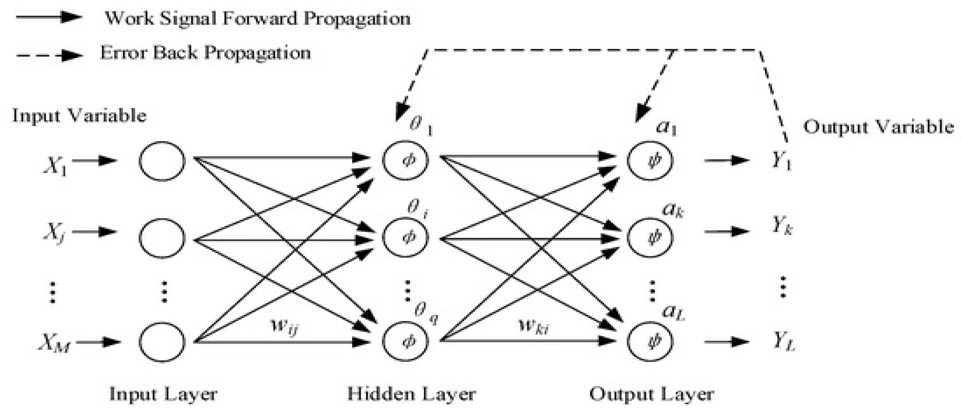
Deep neural network (DNN) consists of the input layer, multiple hidden layers, and the output layer. An error signal defined in Equation (12) needs to be back propagated to adjust the weights between the neurons. When the mean squared error converges, the updating process stops, and the model has been well trained [
44,
45]:
where
n is the number of training samples,
M is the dimensions of input variables,
L is the dimension of output variables,
means the weights from layer
i to layer
j, and
is the intercept. The universal approximation function,
f, needs to be learned to conduct nonlinear fitting. As shown in
Figure 4, the error signal can calculate the best fitted weights and intercepts that can minimize forecasting error. In contrast, the forward working signals can conduct forecasting. Based on the chain rules, the optimal weights and intercepts are derived to form a universal approximation that best defines the relationships between the predictors and the outcome [
45]. Specifically, hyperparameters, such as the number of hidden layers and associated neurons, drop-out rate, activation function (hyperbolic tangent, sigmoid, and ReLu), and optimizer (stochastic decent, gradient decent, AdaDelta, AdaGrad, and etc.), need to be selected in model training. Thereafter, forecasting can be realized in model testing.
3.3. Competitive Analysis
Based on the logistic equation, the Lotka–Volterra model (LVM) is adopted to capture the interactions between competing firms [
14,
18,
23]. Differential equations are given as:
where
can be modeled by adopting users, shipments, revenues, etc.,
denotes the ability of the equation itself,
refers to the limitation of the firm during market expansion,
describes the interaction between the firm and its competitor. In equilibriums, the differential values in Equations (13) and (14) are zeros, and the two objects can be mutually estimated as:
and
. To use discrete data, differential equations are converted into difference equations:
where
,
, and
are used to estimate three important parameters,
.
The original LVM can be generalized to include more objects at a time. For clarity, managerial insights regarding the parameters in LVM are described in
Table 2. The relationships between a firm and its rivals can be one of the six types: pure competition (mutually harmful), mutualism (win-win), predator-prey (win-loss), amensalism (one-side harmful), commensalism (one-side beneficial), and neutralism (independent). Hence, LVM can clearly explain the market dynamics between firms [
18,
19]. Further, stable equilibriums occur when neither of the population levels are changing: differential equations are equal to 0:
,
. In this case, four possible equilibriums,
, are derived: (1)
meaning both species disappear, (2)
meaning specie 1 will survive while specie 2 will disappear, (3)
meaning specie 2 will survive while specie 1 will disappear, and (4)
meaning both species can survive. Each equilibrium point can be stable only if the real parts of the eigenvalues of the Jacobian matrix,
, are negative.
3.4. Performance Assessment
Data envelopment analysis (DEA) is one of the most classic techniques used to measure operational efficiencies among the so-called DMUs (decision management units). There are two common measures [
27]: one is BCC (Banker, Charnes, Cooper) and the other is CCR (Charnes, Cooper, Rhodes). The selection of input and output variables is critical to the efficiency measures and relative performances of the DMUs. Mathematically, operational efficiency for a specific DMU can be expressed as follows:
where
and
are the weights of the input (
) and output (
) variables,
is called non-Archimedean small number, an extremely small positive value that is usually represented by 10
−6, and
i,
r, and
k, respectively, represent indices for input, output, and DMU. The parameter
is used to control variable returns to scale (VRS) in BCC or constant returns to scale (CRS) in CCR (
). For the input-oriented DEA, CCR can be replaced by solving the following formula [
28,
30]:
, subject to
,
,
,
,
. Based on dual theorem in linear programming, the dual form can be solved as follows:
where
and
represent the slack (input excess) and the surplus (output shortfall), and
is a constant ratio of the reduction of input variables used for achieving an efficient DMU.
The main differences between CCR and BCC are VRS or CRS. In simple words, CCR derives operational efficiency (OE) defined by the weighted output over the weighted input. To improve the CRS assumption in CCR, BCC separates OE into two multiplicative parts: scale efficiency (SE) and technical efficiency (TE). Scale efficiency is the ratio of existing inputs (or outputs) of DMUs to the inputs (or outputs) of optimal production scale. Specifically, can be used to justify the trends of returns to scale: means increasing returns to scale (IRS), means constant returns to scale (CRS), and indicates decreasing returns to scale (DRS). If a DMU achieves Pareto efficiency, , it means no adjustment is required (). Otherwise, the required adjustments for an inefficient DMU () are , , where () and () are the input and output variables before (after) adjustment; and are the desired adjustments.
4. Experimental Results
To justify the validity of the presented framework, quarterly sales of the three retailers, Walmart, Costco, and Kroger, are collected from 2005/Q1 to 2021/Q4. For visualization,
Figure 5 displays that Walmart significantly surpasses Costco and Kroger, and all of them demonstrate seasonal variations. To help retail practitioners conduct sales forecasting, economic indicators [
8] are treated as potential predictors. In particular, Lasso is applied to identify key performance indicators. As indicated by
Table 3, CPI and regular wage are commonly identified for the three firms. PPI and oil price are only critical to Walmart because a hypermarket imports lots of goods (fashion clothes, home appliances, furniture, office supplies, sporting goods, electronic appliances, homemade tools, etc.) from foreign manufacturers, and it is more sensitive to the upstream variations. Specifically, DJT are critical to Costco and Kroger because they need frequent freight transportation to support logistics and inventory management. In contrast, GDP are key to Walmart and Costco, while PCE is influential to Walmart and Kroger.
Very interestingly, lots of indicators, such as CCI, PMI, NMI, IMPI, EXPI, etc., are not critical to any of the three firms. Major product categories sold by a firm form a basis for the identified key predictors. Kroger is a chain supermarket selling uncooked food, such as vegetables, fruits, drinks, snacks, fishes, meat, bread, milk, etc., and Costco also sells lots of well-cooked food and bath supplies. According to different product categories sold by the three retailers, Walmart is closer to the upstream (producer) side while Kroger is closer to the downstream (customer) side. In contrast, Costco seems to be close to the median between Walmart and Kroger.
4.1. Forecasting Sales Based on Economic Indicators
After the most significant economic indicators have been identified with respect to the three retail firms, they are treated as the predictors for forecasting sales revenues. To justify the validity of these economic indicators, MARS, SVR, and DNN are compared in sales forecasting. As we know, MARS, SVR, and DNN originate from statistics, quadratic programming, and deep learning. Deep learning algorithms like RNN, GRU, and LSTM are not considered in this research, because they require lots of data samples to optimize their network topologies and the associated hyperparameters. Specifically, the training set (
Table 4) is from 2005/Q1 to 2019/Q4 and the test set is from 2020/Q1 to 2021/Q4 (
Table 5). For all the three firms, it is interesting to observe that SVR exhibits the best performance in the training set, while MARS exhibits the best performance in the test set. Generally, the performances of Costco and Kroger are worse than Walmart, and their MAPEs are slightly greater than 10%. In data science, overfitting means good training performance but poor testing performance. The differences between the training set and the test set are limited, and these results guarantee no overfitting is found in this research.
4.2. Analyzing the Interrelationships
LVM is adopted to analyze interactions between Walmart, Costco, and Kroger. In
Table 6, it is found that the relationship known as
mutualism exists between all pairs. This means that each firm can benefit from the existence of the other retailers. This result may imply the whole retail market is still a growing pie. Since the three firms position themselves in different geographical locations, product categories, and consumer groups, they do not intensively compete with one another.
Table 7 further estimates stable sales equilibriums, considering the interactive dynamics continue. Compared to the sales in 2021/Q4, Costco (+5.9%) and Kroger (+7.8%) significantly increased sales at market equilibriums, while Walmart (−2.8%,) slightly decreased. In
Table 7, the MAPEs for the three retailers are around 10% and these results justify the validity of using LVM in interactive regression. More importantly, they provide a quantitative basis to estimate the degree of change in sales revenues.
In reality, sales revenues are affected by many factors, including manufacturing cost, pricing policies, promotion plans, channel competition, product positioning, geographical location, customer defection, etc. Recently, online e-commerce platforms, such as Amazon, spent lots of resources to compete with traditional retailers. A slogan, “just walk out,” is promoted by Amazon, asking consumers using their smartphone app to pick up their favorite food and simply walk out of the store without having to interact with a cashier. No cashiers are needed to serve on sites because artificial intelligence (AI) technologies automatically detect consumers’ motions and complete all transactions, including bill payments. This paradigm shift deserves observation, in order to evaluate the impact of AI technologies on future developments in the retail industry.
4.3. Deriving Operational Efficiencies and Performance Assessment
To conduct performance assessment, the correlation coefficients between input variables (COGS- cost of goods sold, full-time employees, OE- operating expenses) and the output variable (sales revenue) are shown in
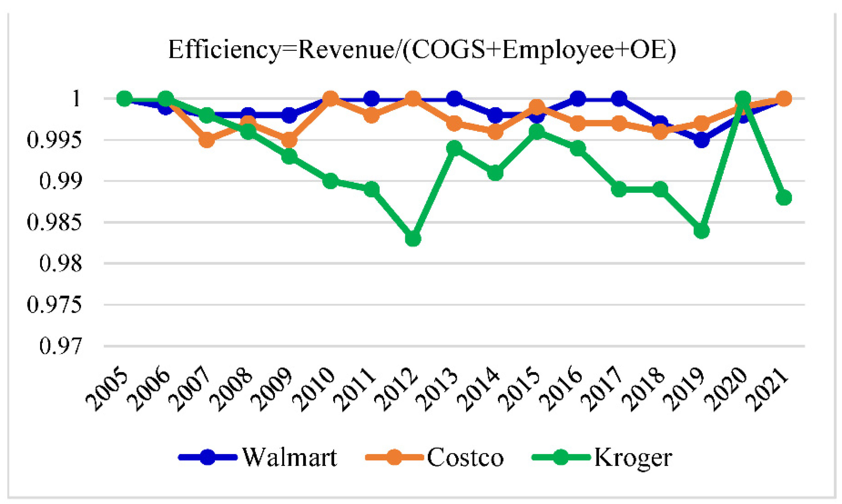
Table 8. Positive coefficients imply that the output is proportional to the input, thus justifying the validity of the input and output variables. In terms of BCC measures, the operational efficiencies for Walmart, Costco, and Kroger are shown in
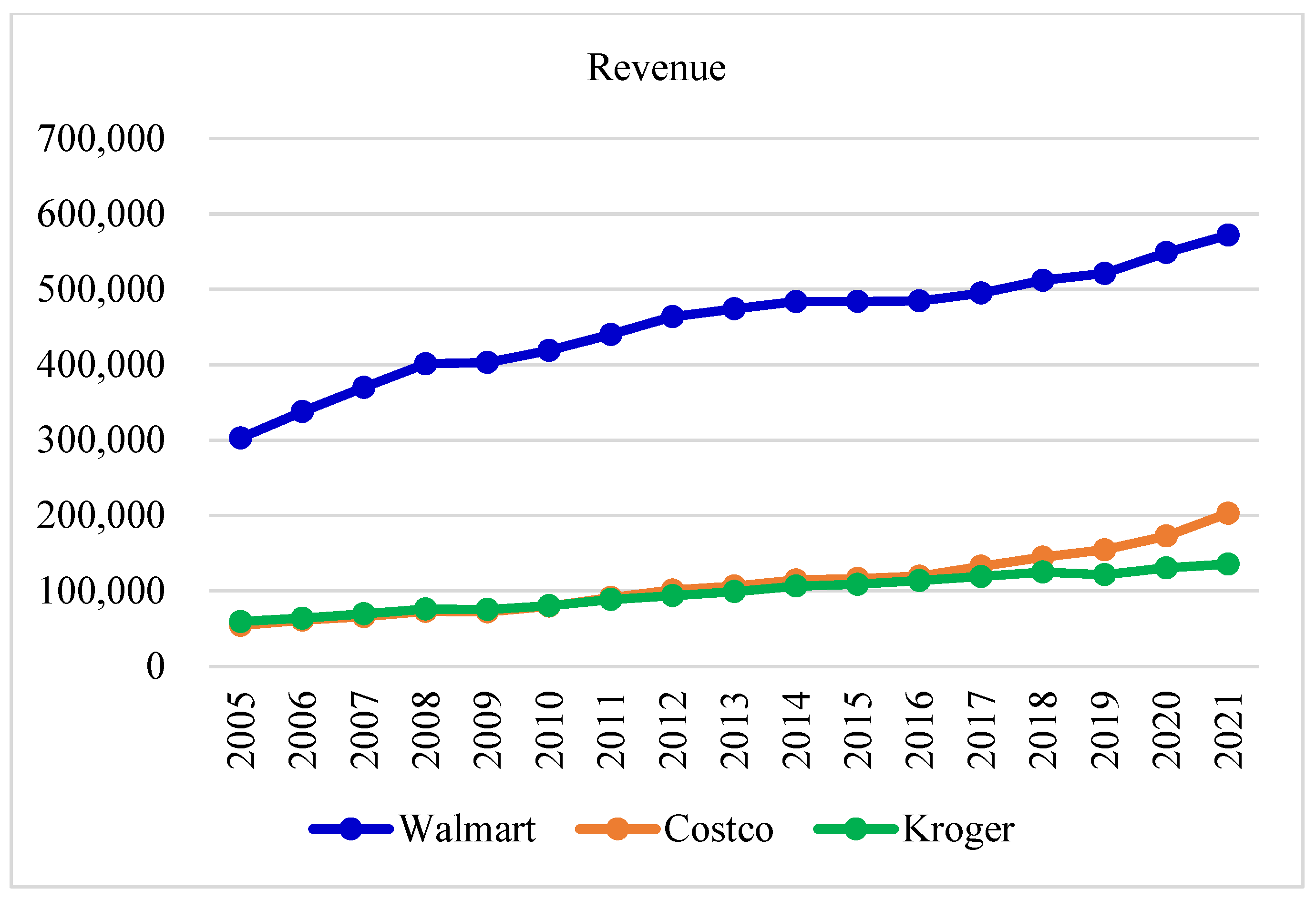
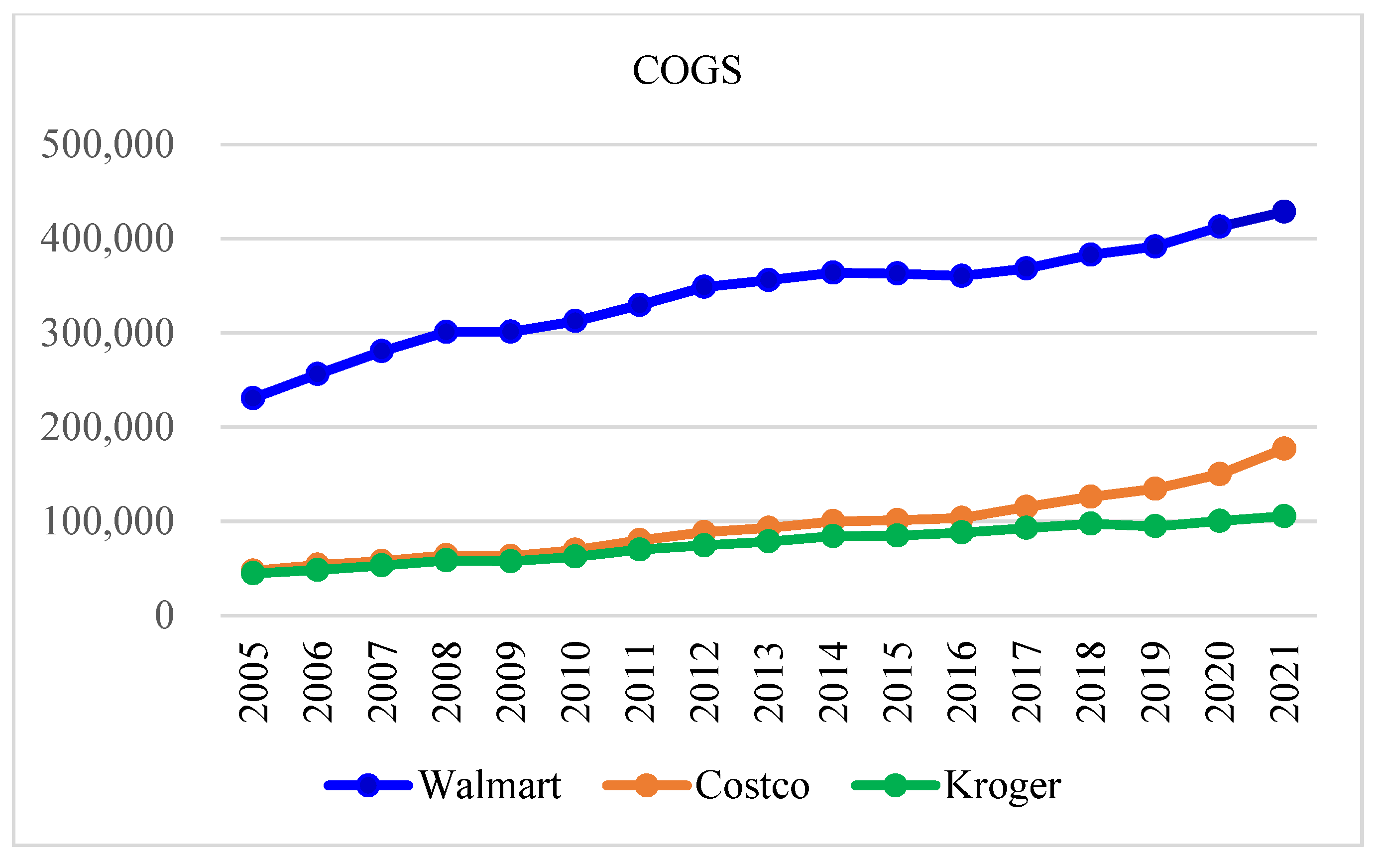
Figure 6. Clearly, Kroger has significantly lagged behind Walmart and Costco since 2009. To address hidden causalities, all input and output variables are displayed in
Figure 7,
Figure 8,
Figure 9 and
Figure 10. Not surprisingly, Walmart exhibits the largest scales of input and output variables. Kroger shows almost equivalent sales (
Figure 7) and COGS (
Figure 8) to Costco, though it has more full-time employees (
Figure 9) and higher operating expenses (
Figure 10) than Costco. These observations clearly account for Kroger’s operational efficiency ranking being the lowest, because it consumes more input resources without generating higher sales revenues. Although Walmart expresses worry about Amazon’s move to retail markets, Kroger can potentially be more impacted by Amazon because it is a chain supermarket with community-based stores. To elicit more insights, partial operational efficiencies with respect to a single input variable are derived and shown in
Table 9: Costco performs poorly in “COGS” and Kroger performs the worst in both “full-time employees” and “operating expenses”.
To help Kroger improve operational efficiencies,
Table 10 shows the required adjustments of input resources in percentages. In 2005, no adjustments were required for any retailer. As shown in
Figure 6, Kroger performed the worst from 2008 to 2019, and hence, it needed to concurrently reduce COGS, full-time employees, and operating expenses during these years. In 2010, 2012, and 2021, Costco and Walmart performed efficiently, and thus, no adjustments were required. Further, the reduction of COGS and operating expenses was more critical to Costco and Kroger, while Walmart seemed to focus on decreasing full-time employees. Although Walmart had the greatest scales of input resources and out revenues, it performed efficiently in many years: 2005, 2010, 2011, 2012, 2013, 2016, 2017, and 2021. In 2018, Walmart spent a lot of money to merge an e-commerce platform because it wanted to defend its territory and compete with Amazon. This event, coupled with the US–China trade war, can explain Walmart’s inefficiencies in 2018 and 2019. On average, Costco did not perform as well as Walmart but it was still more efficient than Kroger. In practice, to enhance operational efficiencies, cost reduction is easier than increasing sales revenues.
5. Discussions
Inspired by the concept of business analytics, this research presents an integrated framework to help retail managers address three critical issues: sales forecasting, market analysis, and performance assessment. Generally, business analytics has four specific modules: descriptive analytics (what happened in the past), diagnostic analytics (why did it happen), predictive analytics (what will happen in the future), and prescriptive analytics (how to take actions to improve shortcomings). Specifically, sales forecasting covers diagnostic analytics and predictive analytics, market analysis covers descriptive analytics and predictive analytics, and performance assessment covers diagnostic analytics and prescriptive analytics. In sales forecasting, CPI and regular wage are identified as two common factors affecting retail sales for Walmart, Costco, and Kroger. The economic indicators used in this research are actually treated as leading signals to retail sales. Due to limited data, quarterly samples are collected from 2005/Q1 to 2021/Q4. However, big events from outside environments, such as the US–China trade war, COVID-19, and inflation since 2022, may impact sales revenues differently. Consequently, more data composed of monthly samples is required in order to justify the research findings.
In market analysis, the relationship known as mutualism is found to exist between the three firms. In other words, a firm can expect to positively vary its sales with its competitors (one increases or decreases, the other has the same direction). Not surprisingly, this finding implies a common driver affecting retail sales. However, in terms of product varieties and market segmentation, Walmart, Costco, and Kroger are not homogeneous. Walmart possesses the greatest variety of products, such as those found in hypermarkets, while Kroger focuses on community supermarkets. In contrast, Costco seems to position itself at the median point between Walmart and Kroger. Thus, to reveal more insights, market analysis should be elaborated to carefully target specific customer groups, and should include product categories and geographic areas. Besides, the results concerning market equilibrium indicate that Kroger has the greatest potential to increase sales. However, this implication does not take the competition from Amazon’s cashier-less stores into account. The paradigm shift arising from artificial intelligence and computer vision deserve observation, in order to evaluate their potential impact on future developments in the retail sector.
Finally, regarding performance assessment, operational efficiencies are mathematically derived by input (resource) and output (outcome) variables. By consulting domain experts, COGS (cost of goods sold), full-time employees, and operating expenses are used as the input, while sales are used as the output. Operational efficiencies are derived annually. As opposed to sales forecasting and market analysis, performance assessment focuses on efficiency: how efficiently does a firm utilize its resources to generate an outcome? As we know, profit margin is usually very low in the retail sector. Thus, to substantially enhance competitive advantage, improvement of operational efficiency may be more important than an increase of sales for retail firms. Possible methods include a decrease of input resources while keeping the same outcome, or the use of the same input resources while generating a higher level of outcome.
6. Conclusions
To help retail firms conduct sales forecasting, market analysis, and performance assessment, this research proposes a novel framework, and the top three US retail firms, Walmart, Costco, and Kroger, are used to evaluate the research validity. More importantly, these three critical issues are surrounded by the concept of business analytics from start to finish. In summary, the research contributions are outlined as follows:
A statistical regression known as Lasso is used to select the economic indicators for Walmart, Costco, and Kroger, and machine learning methods (MARS, SVR, DNN) are used for sales forecasting,
The Lotka–Volterra model is applied to conduct competitive analysis between the top three US retail firms, and to estimate stable market equilibriums in order to reveal insights,
Data envelopment analysis is used to derive operational efficiencies and to indicate the actions required for inefficient firms to improve their input resource variables.
Experimental results show the identified economic indicators incorporated into machine learning work well in sales forecasting (the average MAPEs are below or around 10%). Besides, the demonstrated interrelationship known as mutualism indicates that the total market is still a growing pie, and thus, each firm can benefit alongside the other. Finally, from 2009 to 2019, and also 2021, Kroger performed the worst in operational efficiency. The required improvements suggested include a decrease of full-time employees, a reduction of COGS, and a reduction of operating expenses.
Needless to say, this research is not without limitations: (1) due to limited information, only aggregate sales were collected and analyzed for Walmart, Costco, and Kroger. Product sales with respect to detailed categories (perishable food, home supplies, electronic appliances, snacks, etc.) could provide more insights [
4]; (2) only onsite retailers with branch stores were analyzed and compared, while the competition arising from online e-commerce platforms, such as Amazon, were omitted. Moving forward, the boundary between onsite stores and online platforms is expected to blur, and hence, their competition deserves to be addressed [
2,
31]; and (3) the STP issue, market segmentation, customer targeting, and product positioning should be considered in order to fit consumer preferences for the accomplishment of upselling and cross selling. Furthermore, purchasing transaction records should be linked to customer demographics to develop attractive product strategies and promotion plans.


