
A System for Sustainable Usage of Computing Resources Leveraging Deep Learning Predictions


Abstract
:Featured Application
Abstract
1. Introduction
- The paper describes the process of gathering live metrics from distributed applications running on a Kubernetes [4] cluster, inspiring itself from a real production system deployed at the European Laboratory for Nuclear Physics (CERN). Kubernetes runs containers based on snapshots (called images). The most famous container orchestration platform that Kubernetes can run on is [5].
- A few different modern techniques of analyzing and forecasting time-series data are presented and compared with more traditional approaches.
- The performance of the different forecasting algorithms is presented, showcasing which ones are more applicable to the specific use-case presented in this paper, CPU usage forecasting.
- An experiment is conducted based on the algorithm found to be the best performer. The results from the experiment allow us to understand and quantify the potential energy-saving benefits of using this implementation. We compare the ideal scenario with the predictions provided on the validation data, with encouraging results.
2. Materials and Methods
2.1. Automatic Resource Cluster Scaling
2.2. Time-Series Analysis
2.3. Deep Learning Models for Time-Series Analysis
- Vision and image identification through the pioneering work of Yann LeCun in automatic zip code identification off postal packages [15];
- Speech recognition through the usage of convolutional neural networks [16];
- Complex learning tasks through q-learning and reinforcement learning, coming closer to top human-level performance in tasks such as playing video games [17].
2.4. The Environmental Impact of Computing
3. System Setup and Deep Learning Algorithms
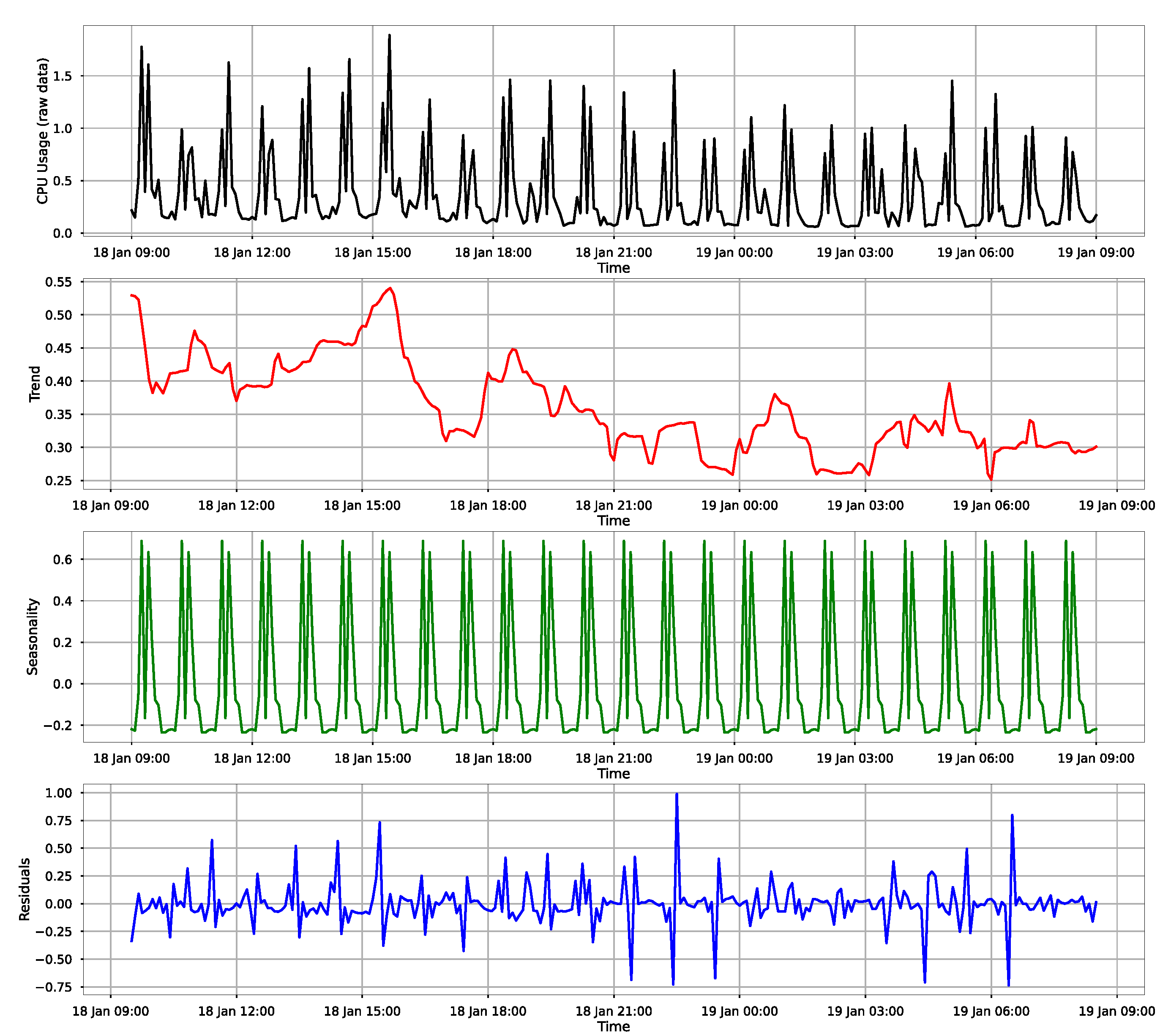
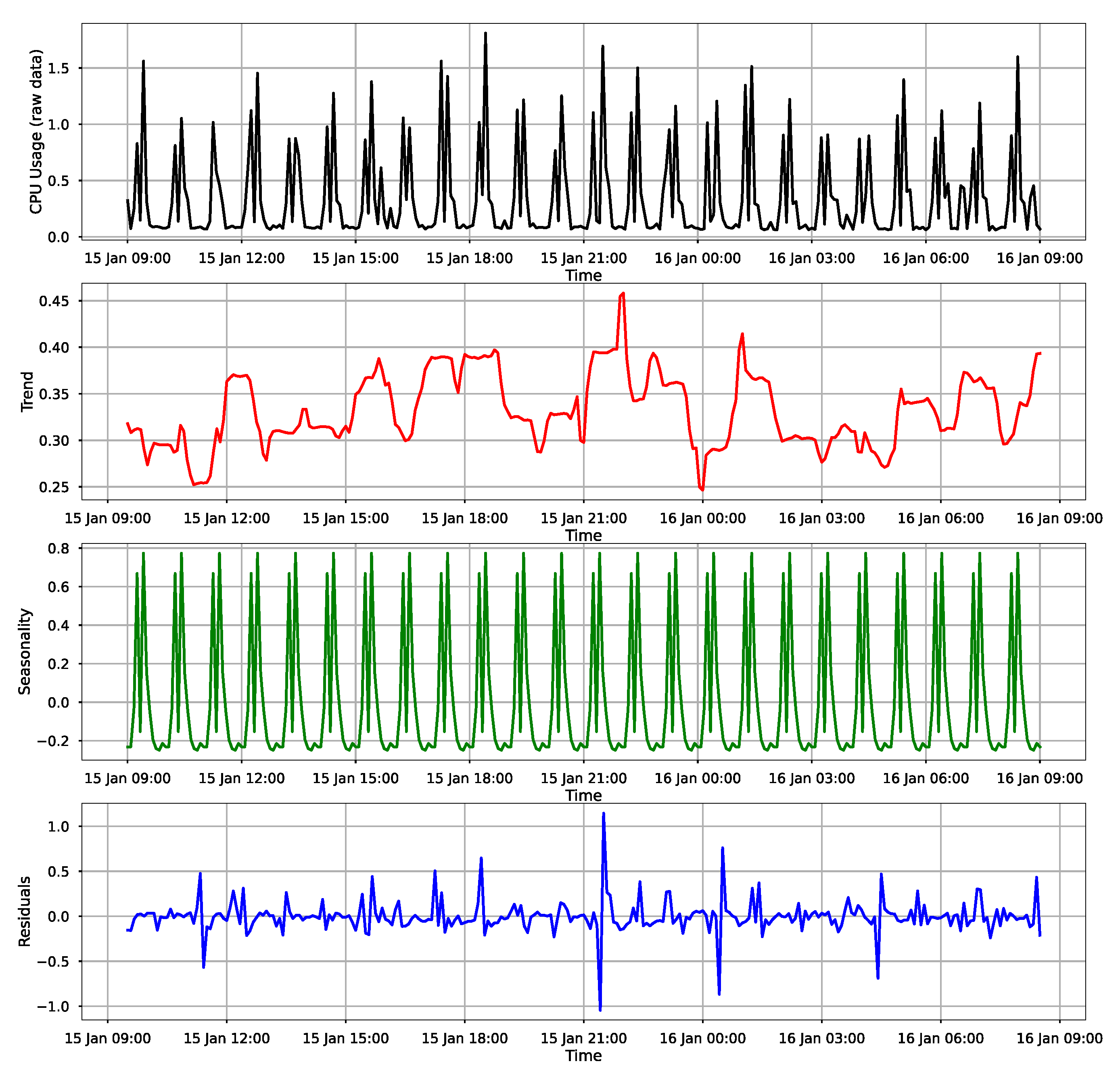
3.1. Overview
- Trend—if the data are increasing or decreasing in the long term.
- Seasonality—if certain periodic changes occur in the data and can be spotted by removing the other pieces of data.
- Residuals—the noise in the data which can be represented in this case by ad-hoc users of the API which cause some load on the systems, or other anomalies.
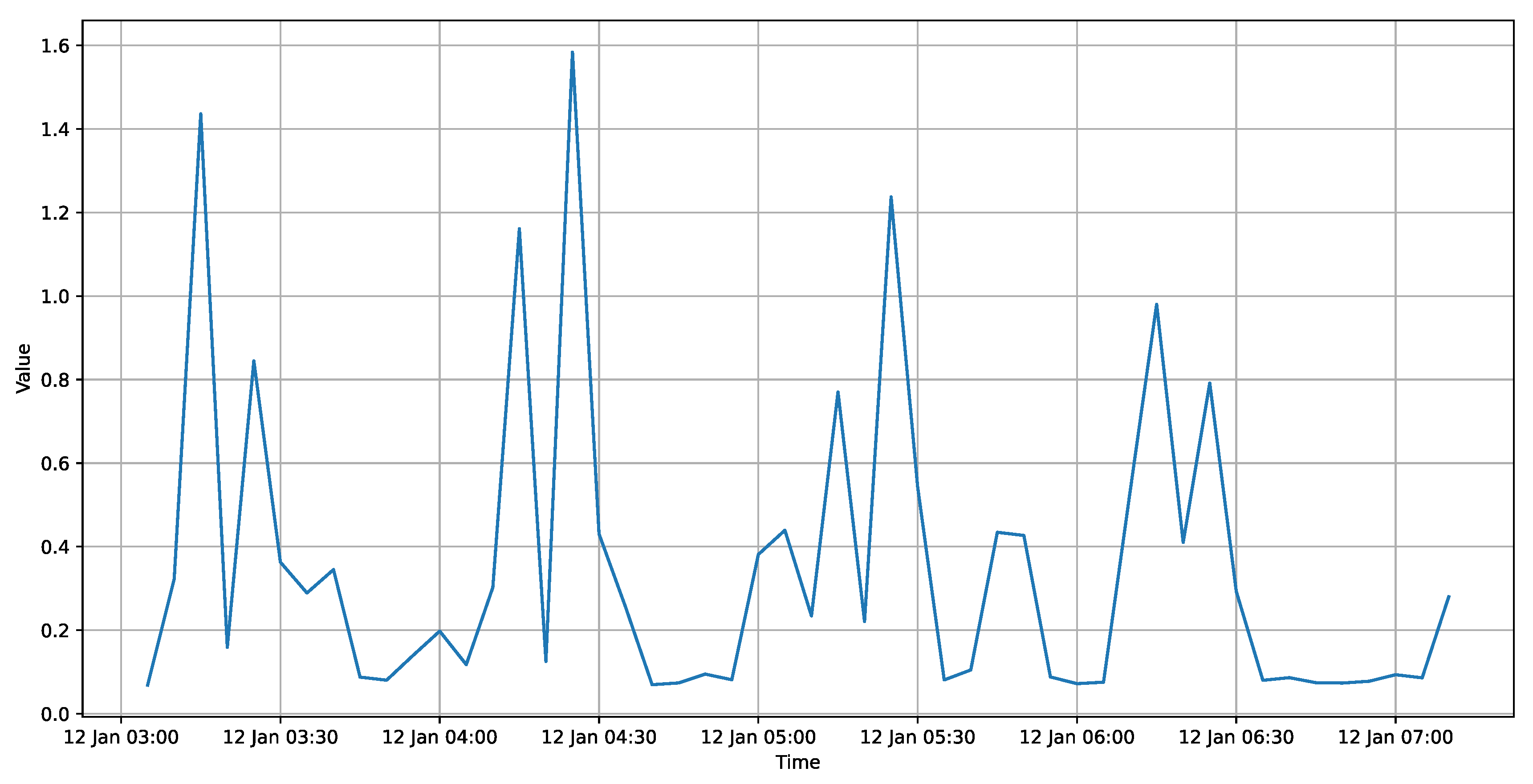
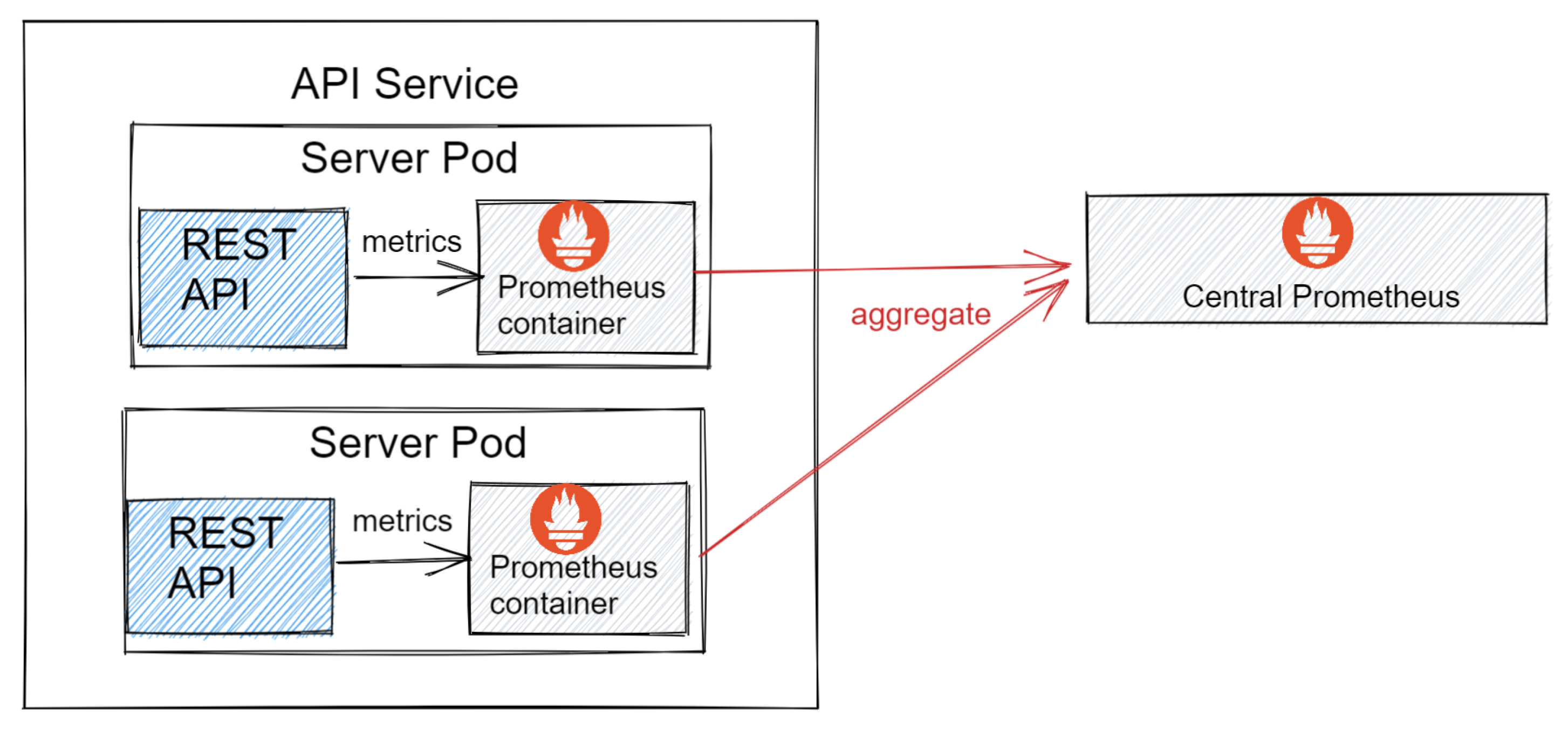
3.2. System Architecture and Data Collection
| Listing 1. Prometheus query for collecting the data. |
| sum(rate( process_cpu_seconds_total{ kubernetes_namespace =~ "api-process"}[5m] ) ) |
| Listing 2. Aggregated data from Prometheus. |
| { "resultType": "matrix", "result": [ { "metric": {}, "values": [ [1641773100, "0.08205714228572106"] ]}] } |
3.3. Classical Time Series Analysis Algorithms
- p—controls the auto regression (AR) part of the algorithm.
- d—controls the differencing (I) part of the algorithm, the number of non-seasonal differences.
- q—controls the moving average (MA) part of the algorithm, the number of lagged forecast errors.
- p—[0, 1, 2, 4, 6, 8, 10];
- d—[0, 1, 2, 3];
- q—[0, 1, 2, 3].
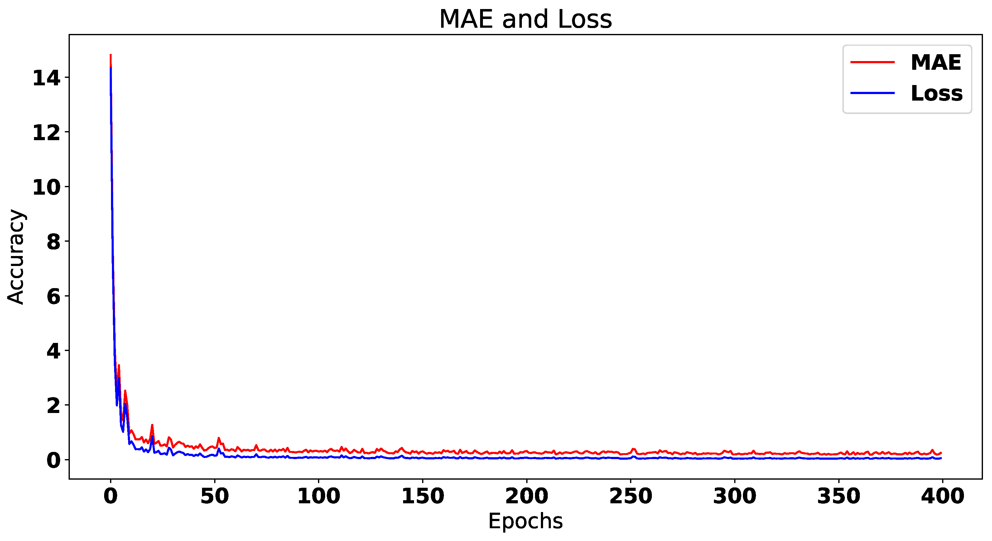
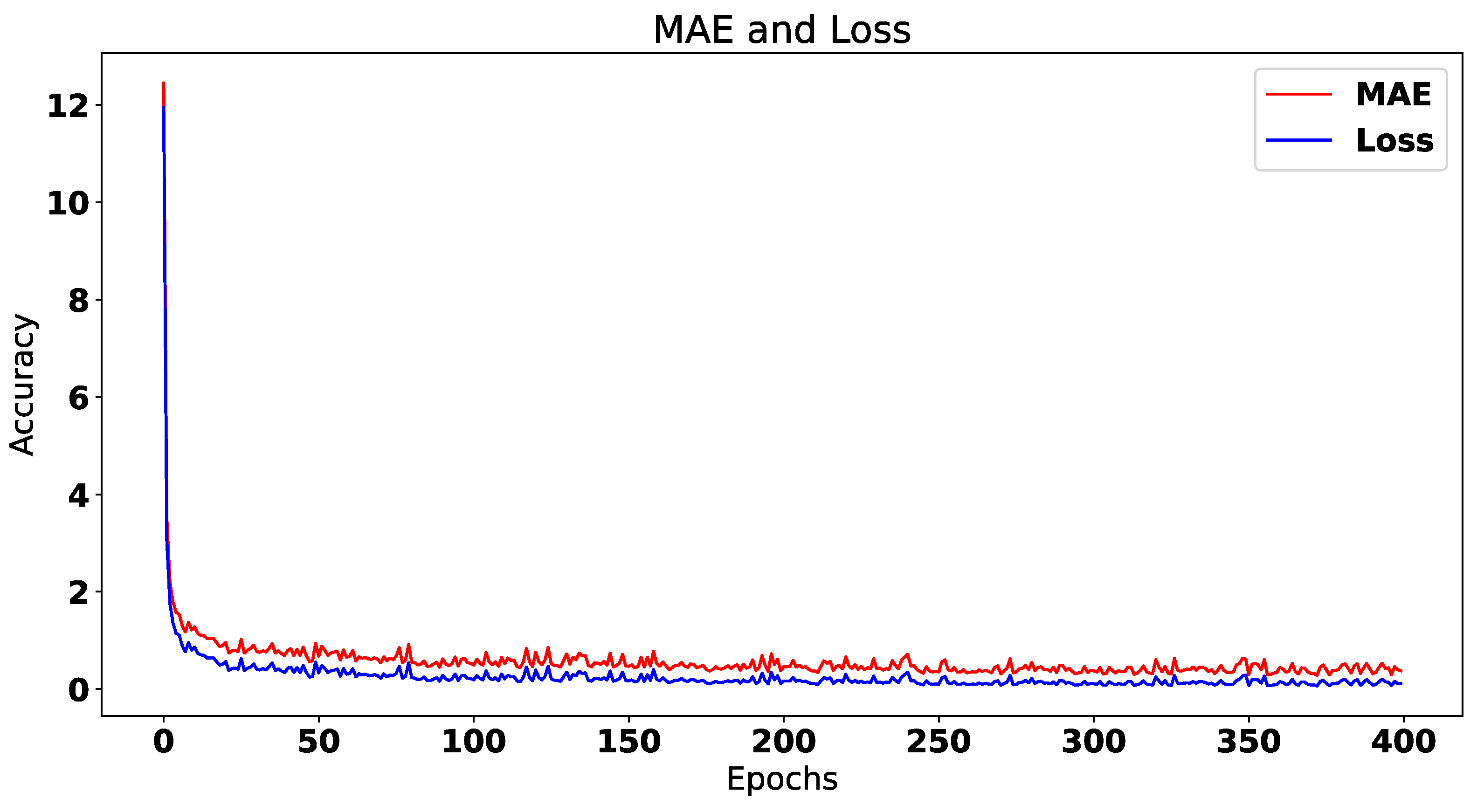
3.4. Deep Learning Algorithms
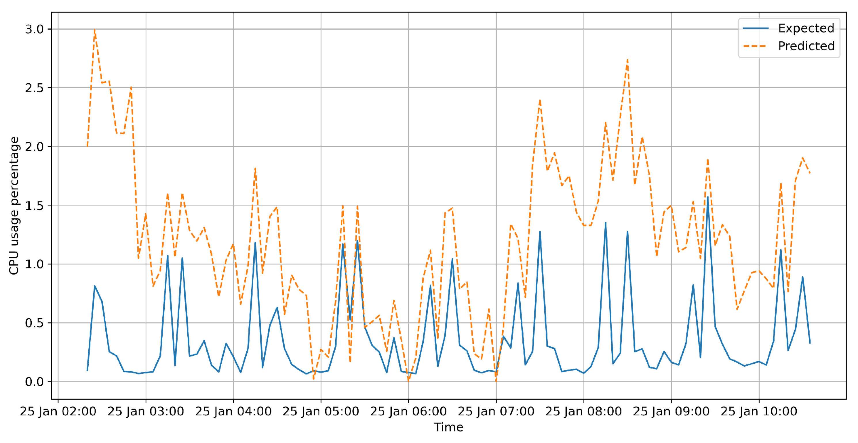
- Convolutional neural network (CNN) model—3 layers of 1-dimensional convolutions followed by a batch normalization layer and a rectified linear unit layer to apply non-linear transformation to the data. The resulting tensors are passed through a last pooling layer that averages the results of the convolutions and is fed into a 1-neuron dense layer that outputs a predicted value.
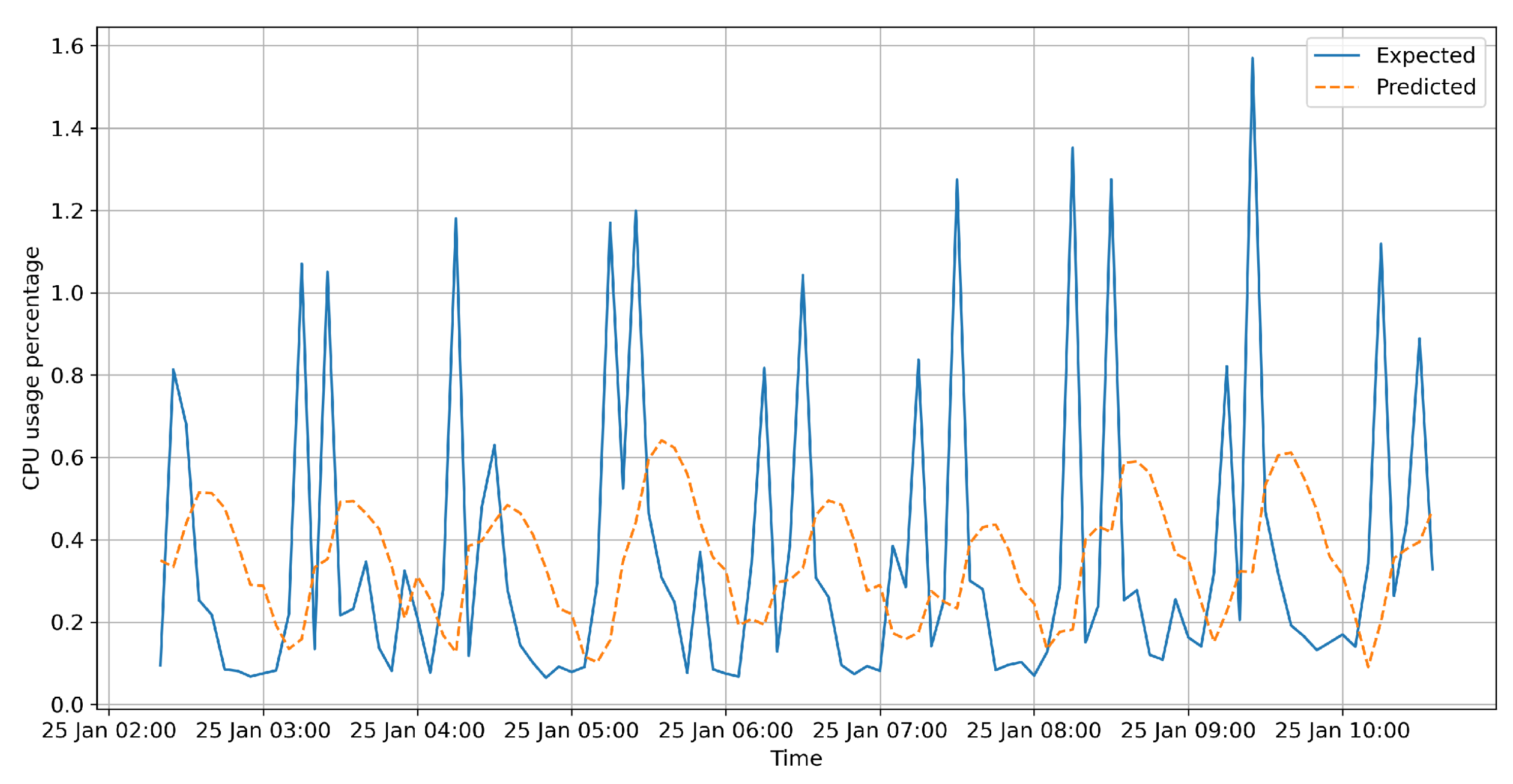
- Recurring neural network (RNN) model—2 layers of a simple recurring neural network are used in order to train the model, the first layer feeding a sequence into the second one, then passing the information to a fully-connected dense neural network layer.
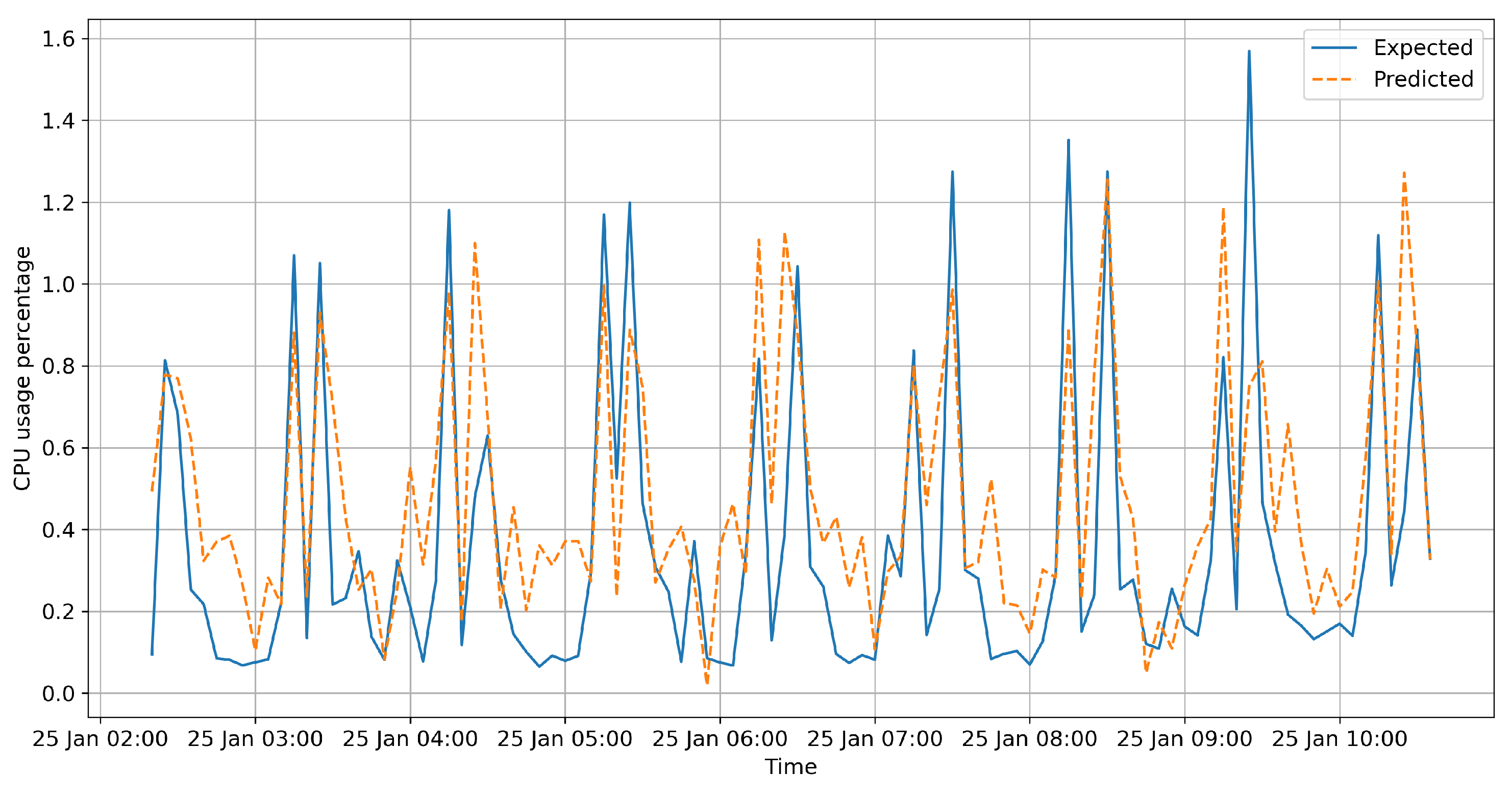
- Long short-term memory (LSTM) model—2 layers of an LSTM based neural network, using specialized recurring neural network cells that have a special memory layer feeding into each of the neurons in the sequence. The layers both return sequences and feed into another pair of dense neural network layers before outputting a prediction.
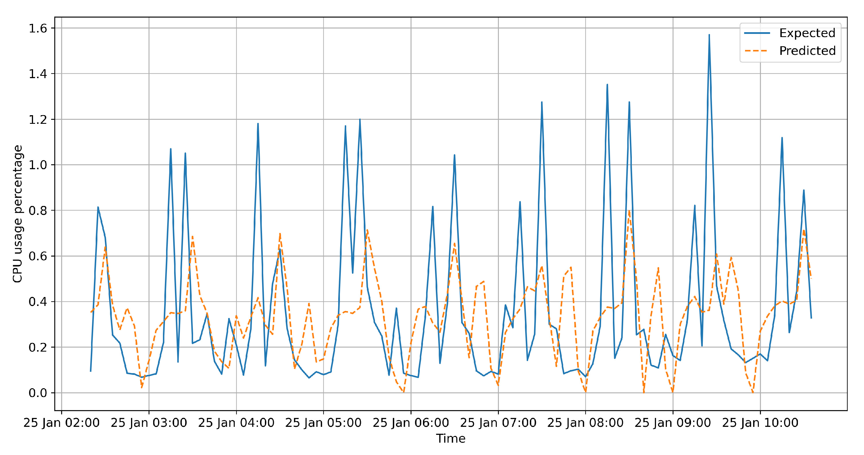
4. Results
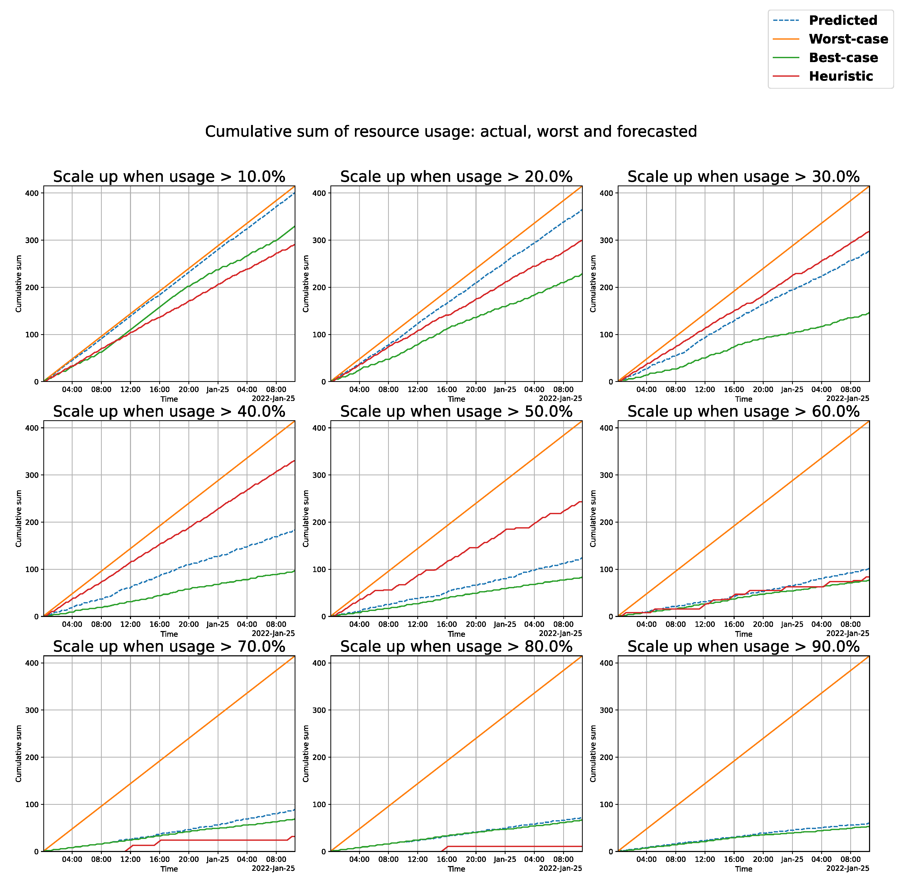
Resource Usage Impact
- Ratio—the CPU usage over which the system should scale up.
- Real Over—the number of real instances in which the CPU usage surpassed the value (training + test data).
- Forecast Over—the number of forecasts where the CPU usage is above the ratio value.
- Real All % Over—the percentage of real predictions where the CPU usage values were over the ratio.
- All % Over—the percentage of forecasts where the CPU usage values were over the ratio.
- Val. Real Over—the number of real instances where the values where over the ratio in the validation data.
- Val. Over—the number of forecast instances where the values where over the ratio in the validation data.
- Val. Real %—the percentage of real measurements where the CPU usage values were over the ratio in the validation data.
- Val.%—the percentage of forecasts where the CPU usage values were over the ratio in the validation data.
- Orange—the worst-case scenario (identical for every instance), where the system is constantly in high CPU-usage mode.
- Green—the best-case scenario, matching the real CPU resource usage. The ideal scaling system would already know if the CPU usage will be above the threshold in the next 5 min, scaling up before the load occurs.
- Blue—the scenario where prediction values larger than the ratio are considered “scale up” commands.
- Red—a simple heuristic that mimics what a traditional resource scheduler would do. It takes the previous 2 measurements and compares it to the current timestamp. If the difference between the mean of the previous 2 measurements and the current reading is larger than the “ratio”, a scale up is issued. Alternatively, if the difference between the current value and the previous means is smaller by ratio %, a scale down is issued.
5. Conclusions
Author Contributions
Funding
Institutional Review Board Statement
Informed Consent Statement
Data Availability Statement
Conflicts of Interest
Abbreviations
| CNN | Convolutional neural network |
| LSTM | Long-short term memory |
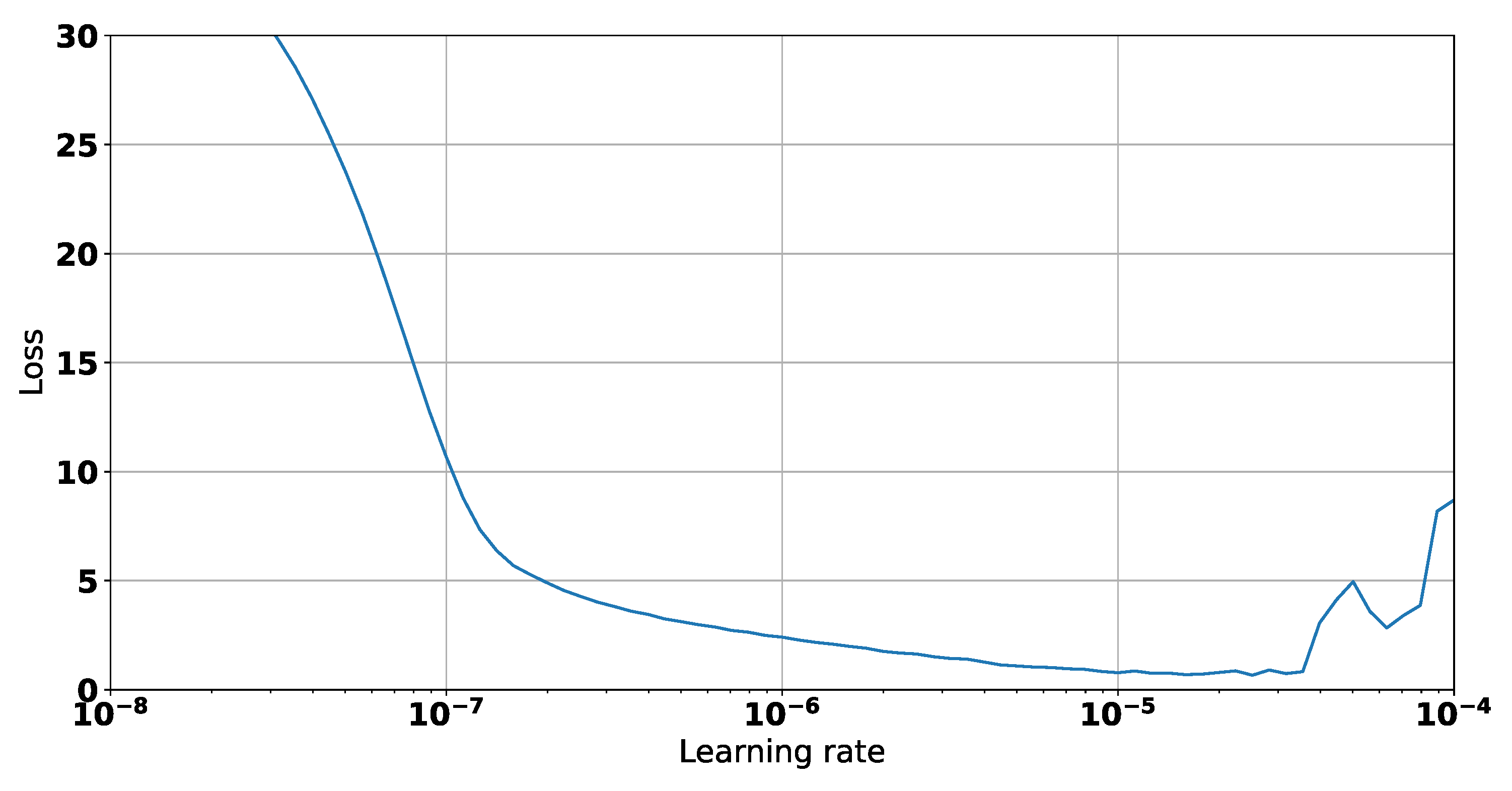
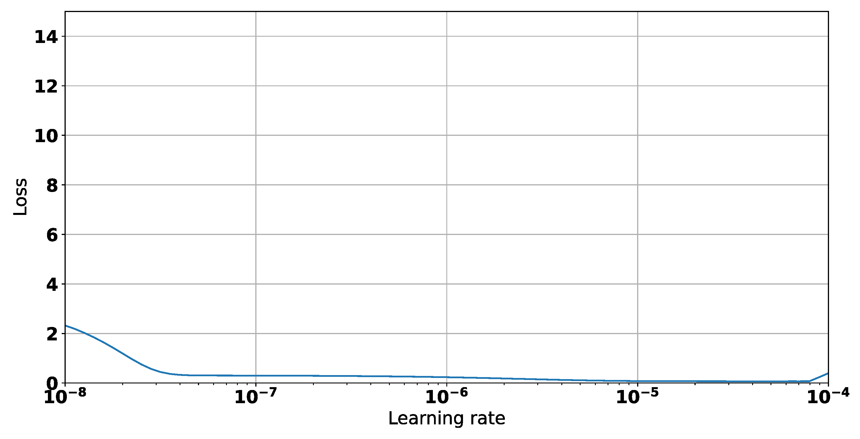
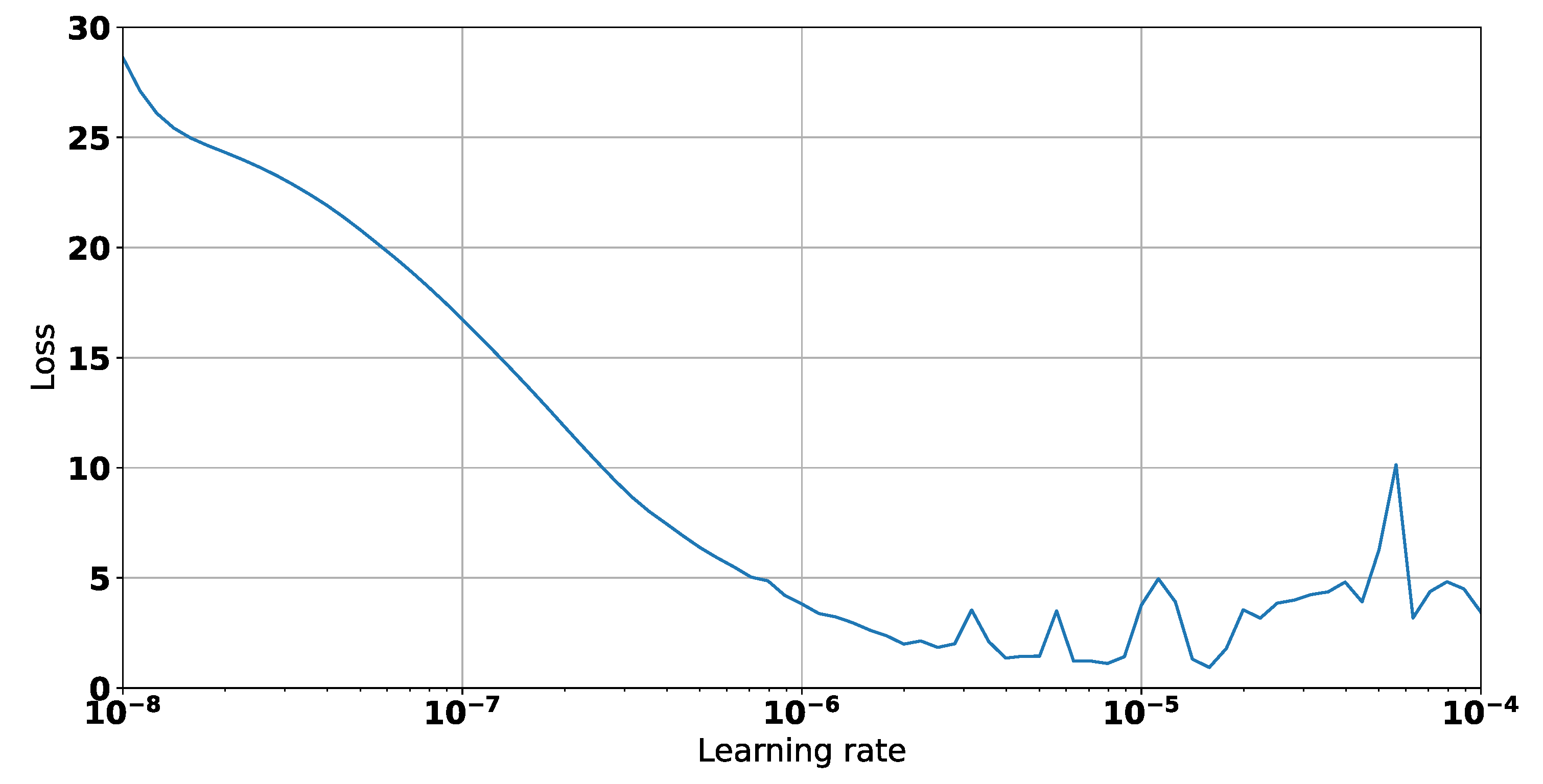
| LR | Learning rate |
| RNN | Recurrent neural network |
| API | Application programmer interface |
| CPU | Central processing unit |
| CERN | The European Organization for Particle Physics |
References
- Pai, P.F.; Lin, C.S. A hybrid ARIMA and support vector machines model in stock price forecasting. Omega 2005, 33, 497–505. [Google Scholar] [CrossRef]
- Duggan, M.; Mason, K.; Duggan, J.; Howley, E.; Barrett, E. Predicting host CPU utilization in cloud computing using recurrent neural networks. In Proceedings of the 2017 12th International Conference for Internet Technology and Secured Transactions (ICITST), Cambridge, UK, 11–14 December 2017; IEEE: Piscataway, NJ, USA, 2017; pp. 67–72. [Google Scholar]
- Qiu, F.; Zhang, B.; Guo, J. A deep learning approach for VM workload prediction in the cloud. In Proceedings of the 2016 17th IEEE/ACIS International Conference on Software Engineering, Artificial Intelligence, Networking and Parallel/Distributed Computing (SNPD), Shanghai, China, 30 May–1 June 2016; IEEE: Piscataway, NJ, USA, 2016; pp. 319–324. [Google Scholar]
- Kubernetes Documentation. Available online: https://kubernetes.io/docs/home/ (accessed on 6 July 2022).
- Docker Container Platform. Available online: https://docs.docker.com/get-started/overview/ (accessed on 6 July 2022).
- Gulli, A.; Pal, S. Deep Learning with Keras; Packt Publishing Ltd.: Birmingham, UK, 2017. [Google Scholar]
- Pandas Data Analysis Library. Available online: https://pandas.pydata.org/ (accessed on 6 July 2022).
- Luksa, M. Kubernetes in Action; Simon and Schuster: New York, NY, USA, 2017. [Google Scholar]
- Verma, A.; Pedrosa, L.; Korupolu, M.; Oppenheimer, D.; Tune, E.; Wilkes, J. Large-scale cluster management at Google with Borg. In Proceedings of the Tenth European Conference on Computer Systems, Bordeaux, France, 21–24 April 2015; pp. 1–17. [Google Scholar]
- Balla, D.; Simon, C.; Maliosz, M. Adaptive scaling of Kubernetes pods. In Proceedings of the NOMS 2020—2020 IEEE/IFIP Network Operations and Management Symposium, Budapest, Hungary, 20–24 April 2020; IEEE: Piscataway, NJ, USA, 2020; pp. 1–5. [Google Scholar]
- Knative Scaler. Available online: https://github.com/knative/docs (accessed on 6 July 2022).
- Rattihalli, G.; Govindaraju, M.; Lu, H.; Tiwari, D. Exploring potential for non-disruptive vertical auto scaling and resource estimation in kubernetes. In Proceedings of the 2019 IEEE 12th International Conference on Cloud Computing (CLOUD), Milan, Italy, 8–13 July 2019; IEEE: Piscataway, NJ, USA, 2019; pp. 33–40. [Google Scholar]
- Toka, L.; Dobreff, G.; Fodor, B.; Sonkoly, B. Machine learning-based scaling management for kubernetes edge clusters. IEEE Trans. Netw. Serv. Manag. 2021, 18, 958–972. [Google Scholar] [CrossRef]
- Zhang, G.P. Time series forecasting using a hybrid ARIMA and neural network model. Neurocomputing 2003, 50, 159–175. [Google Scholar] [CrossRef]
- LeCun, Y.; Boser, B.; Denker, J.S.; Henderson, D.; Howard, R.E.; Hubbard, W.; Jackel, L.D. Backpropagation applied to handwritten zip code recognition. Neural Comput. 1989, 1, 541–551. [Google Scholar] [CrossRef]
- Abdel-Hamid, O.; Mohamed, A.R.; Jiang, H.; Deng, L.; Penn, G.; Yu, D. Convolutional neural networks for speech recognition. IEEE/ACM Trans. Audio Speech Lang. Process. 2014, 22, 1533–1545. [Google Scholar] [CrossRef]
- Vinyals, O.; Babuschkin, I.; Czarnecki, W.M.; Mathieu, M.; Dudzik, A.; Chung, J.; Choi, D.H.; Powell, R.; Ewalds, T.; Georgiev, P.; et al. Grandmaster level in StarCraft II using multi-agent reinforcement learning. Nature 2019, 575, 350–354. [Google Scholar] [CrossRef]
- Livieris, I.E.; Pintelas, E.; Pintelas, P. A CNN–LSTM model for gold price time-series forecasting. Neural Comput. Appl. 2020, 32, 17351–17360. [Google Scholar] [CrossRef]
- Lawrence, S.; Giles, C.L.; Tsoi, A.C.; Back, A.D. Face recognition: A convolutional neural-network approach. IEEE Trans. Neural Netw. 1997, 8, 98–113. [Google Scholar] [CrossRef]
- Haq, M.A.; Jilani, A.K.; Prabu, P. Deep Learning Based Modeling of Groundwater Storage Change. CMC-Comput. Mater. Contin. 2021, 70, 4599–4617. [Google Scholar]
- Haq, M.A. Smotednn: A novel model for air pollution forecasting and aqi classification. Comput. Mater. Contin. 2022, 71, 1. [Google Scholar]
- Werbos, P.J. Backpropagation through time: What it does and how to do it. Proc. IEEE 1990, 78, 1550–1560. [Google Scholar] [CrossRef]
- Gruslys, A.; Munos, R.; Danihelka, I.; Lanctot, M.; Graves, A. Memory-efficient backpropagation through time. Adv. Neural Inf. Process. Syst. 2016, 29, 1–9. [Google Scholar]
- Rao, S.N.; Shobha, G.; Prabhu, S.; Deepamala, N. Time Series Forecasting methods suitable for prediction of CPU usage. In Proceedings of the 2019 4th International Conference on Computational Systems and Information Technology for Sustainable Solution (CSITSS), Bengaluru, India, 20–21 December 2019; IEEE: Piscataway, NJ, USA, 2019; Volume 4, pp. 1–5. [Google Scholar]
- Siami-Namini, S.; Namin, A.S. Forecasting economics and financial time series: ARIMA vs. LSTM. arXiv 2018, arXiv:1803.06386. [Google Scholar]
- Sagheer, A.; Kotb, M. Time series forecasting of petroleum production using deep LSTM recurrent networks. Neurocomputing 2019, 323, 203–213. [Google Scholar] [CrossRef]
- Qin, Y.; Song, D.; Chen, H.; Cheng, W.; Jiang, G.; Cottrell, G. A dual-stage attention-based recurrent neural network for time series prediction. arXiv 2017, arXiv:1704.02971. [Google Scholar]
- Patterson, D.; Gonzalez, J.; Hölzle, U.; Le, Q.; Liang, C.; Munguia, L.M.; Rothchild, D.; So, D.R.; Texier, M.; Dean, J. The carbon footprint of machine learning training will plateau, then shrink. Computer 2022, 55, 18–28. [Google Scholar] [CrossRef]
- Fridgen, G.; Körner, M.F.; Walters, S.; Weibelzahl, M. Not all doom and gloom: How energy-intensive and temporally flexible data center applications may actually promote renewable energy sources. Bus. Inf. Syst. Eng. 2021, 63, 243–256. [Google Scholar] [CrossRef]
- Nakamoto, S. Bitcoin: A peer-to-peer electronic cash system. Decentralized Bus. Rev. 2008, 4, 21260. [Google Scholar]
- Farsi, B.; Amayri, M.; Bouguila, N.; Eicker, U. On short-term load forecasting using machine learning techniques and a novel parallel deep LSTM-CNN approach. IEEE Access 2021, 9, 31191–31212. [Google Scholar] [CrossRef]
- Wu, D.; Wu, C. Research on the Time-Dependent Split Delivery Green Vehicle Routing Problem for Fresh Agricultural Products with Multiple Time Windows. Agriculture 2022, 12, 793. [Google Scholar] [CrossRef]
- Liu, L.; Wang, H.; Liu, X.; Jin, X.; He, W.B.; Wang, Q.B.; Chen, Y. GreenCloud: A new architecture for green data center. In Proceedings of the 6th International Conference Industry Session on Autonomic Computing and Communications Industry Session, Barcelona, Spain, 15 June 2009; pp. 29–38. [Google Scholar]
- Statsmodels Data Analysis Library. Available online: https://www.statsmodels.org/stable/index.html (accessed on 7 August 2022).
- Turnbull, J. Monitoring with Prometheus. Turnbull Press. 2018. Available online: https://www.prometheusbook.com/MonitoringWithPrometheus_sample.pdf (accessed on 19 August 2022).
- Chen, L.; Xian, M.; Liu, J. Monitoring System of OpenStack Cloud Platform Based on Prometheus. In Proceedings of the 2020 International Conference on Computer Vision, Image and Deep Learning (CVIDL), Chongqing, China, 10–12 July 2020; IEEE: Piscataway, NJ, USA, 2020; pp. 206–209. [Google Scholar]
- Martin, A.; Ashish, A.; Paul, B.; Eugene, B.; Chen, Z.; Citro, C.; Corrado, G.S.; Davis, A.; Dean, J.; Devin, M. TensorFlow: Large-Scale Machine Learning on Heterogeneous Distributed Systems. 2015. Available online: https://www.tensorflow.org/ (accessed on 6 July 2022).
- Balasundaram, S.; Prasad, S.C. Robust twin support vector regression based on Huber loss function. Neural Comput. Appl. 2020, 32, 11285–11309. [Google Scholar] [CrossRef]
- Pries, R.; Jarschel, M.; Schlosser, D.; Klopf, M.; Tran-Gia, P. Power consumption analysis of data center architectures. In Proceedings of the International Conference on Green Communications and Networking, Colmar, France, 5–7 October 2011; Springer: Berlin/Heidelberg, Germany, 2011; pp. 114–124. [Google Scholar]


| Architecture | No. Parameters | Optimal LR |
|---|---|---|
| CNN | 25,793 | |
| LSTM + DNN | 17,573 | |
| RNN | 4961 |
| Layer | Parameters |
|---|---|
| lambda (Lambda) | 0 |
| simple_rnn (SimpleRNN) | 1680 |
| simple_rnn_1 (SimpleRNN) | 3240 |
| dense (Dense) | 41 |
| lambda_1 (Lambda) | 0 |
| Layer | Parameters |
|---|---|
| lambda (Lambda) | 0 |
| conv1d (Conv1D) | 256 |
| batch_normalization | 256 |
| re_lu (ReLU) | 0 |
| conv1d_1 (Conv1D) | 12,352 |
| batch_normalization_1 | 256 |
| re_lu_1 (ReLU) | 0 |
| conv1d_2 (Conv1D) | 12,352 |
| batch_normalization_2 | 256 |
| re_lu_2 (ReLU) | 0 |
| global_average_pooling1d | 0 |
| dense (Dense) | 65 |
| lambda_1 (Lambda) | 0 |
| Layer | Parameters |
|---|---|
| lambda (Lambda) | 0 |
| bidirectional | 33,792 |
| bidirectional_1 | 41,216 |
| dense (Dense) | 65 |
| lambda_1 (Lambda) | 0 |
| Architecture | Training Time/Epoch | Val. MAE | Val. Loss |
|---|---|---|---|
| CNN | 8 ms | 0.8446 | 0.1265 |
| LSTM + DNN | 9 ms | 0.2175 | 0.0475 |
| RNN | 1 s 29 ms | 0.1653 | 0.0843 |
| ARIMA | N/A | 0.2384 | N/A |
| Ratio | Real Over | Forecast Over | Real All % Over | All % Over | Val. Real Over | Val. Over | Val. Real % | Val. % | |
|---|---|---|---|---|---|---|---|---|---|
| 0 | 0.1 | 3216 | 4072 | 72.8 | 92.2 | 330 | 390 | 79.5 | 94.0 |
| 1 | 0.2 | 2173 | 3397 | 49.2 | 76.9 | 229 | 331 | 55.2 | 79.8 |
| 2 | 0.3 | 1517 | 2349 | 34.4 | 53.2 | 147 | 232 | 35.4 | 55.9 |
| 3 | 0.4 | 1049 | 1580 | 23.8 | 35.8 | 97 | 156 | 23.4 | 37.6 |
| 4 | 0.5 | 891 | 1171 | 20.2 | 26.5 | 83 | 113 | 20.0 | 27.2 |
| 5 | 0.6 | 808 | 975 | 18.3 | 22.1 | 77 | 92 | 18.6 | 22.2 |
| 6 | 0.7 | 731 | 843 | 16.6 | 19.1 | 69 | 83 | 16.6 | 20.0 |
| 7 | 0.8 | 654 | 706 | 14.8 | 16.0 | 67 | 66 | 16.1 | 15.9 |
| 8 | 0.9 | 537 | 548 | 12.2 | 12.4 | 53 | 51 | 12.8 | 12.3 |
| Ratio | Worst | Forecast | Ideal | % From Worst | % From Ideal | |
|---|---|---|---|---|---|---|
| 0 | 0.1 | 415 | 390 | 330 | 94.0 | 118.2 |
| 1 | 0.2 | 415 | 331 | 229 | 79.8 | 144.5 |
| 2 | 0.3 | 415 | 232 | 147 | 55.9 | 157.8 |
| 3 | 0.4 | 415 | 156 | 97 | 37.6 | 160.8 |
| 4 | 0.5 | 415 | 113 | 83 | 27.2 | 136.1 |
| 5 | 0.6 | 415 | 92 | 77 | 22.2 | 119.5 |
| 6 | 0.7 | 415 | 83 | 69 | 20.0 | 120.3 |
| 7 | 0.8 | 415 | 66 | 67 | 15.9 | 98.5 |
| 8 | 0.9 | 415 | 51 | 53 | 12.3 | 96.2 |
Publisher’s Note: MDPI stays neutral with regard to jurisdictional claims in published maps and institutional affiliations. |
© 2022 by the authors. Licensee MDPI, Basel, Switzerland. This article is an open access article distributed under the terms and conditions of the Creative Commons Attribution (CC BY) license (https://creativecommons.org/licenses/by/4.0/).
Share and Cite
Cioca, M.; Schuszter, I.C. A System for Sustainable Usage of Computing Resources Leveraging Deep Learning Predictions. Appl. Sci. 2022, 12, 8411. https://doi.org/10.3390/app12178411
Cioca M, Schuszter IC. A System for Sustainable Usage of Computing Resources Leveraging Deep Learning Predictions. Applied Sciences. 2022; 12(17):8411. https://doi.org/10.3390/app12178411
Chicago/Turabian StyleCioca, Marius, and Ioan Cristian Schuszter. 2022. "A System for Sustainable Usage of Computing Resources Leveraging Deep Learning Predictions" Applied Sciences 12, no. 17: 8411. https://doi.org/10.3390/app12178411