Thermal Modelling and Experimental Validation in the Perspective of Tool Steel Laser Polishing

Abstract

Laser polishing (LP) is a process that allows a significant reduction of the surface roughness of a metal workpiece via re-melting a shallow layer of material. However, the practical use of LP is limited due to the difficulty of satisfying the high surface polishing quality for industries such as jewelry. Hence, this study presents a thermal model based on the Chernoff formula for fixed and moving LP processes. The model was validated via a sensitivity analysis of the coefficient of absorption of the solid and liquid phase and through comparing the results with the corresponding experimental observations of the melt pools produced. In this investigation, a continuous wave, high power diode laser (980 nm wavelength, Ø 0.9 mm spot size with a flat top distribution) was coupled to a fixed focusing head. The material was a hardened tool steel (X38CrMVo5-1 steel-1.2343) with an initial surface state obtained by electrical discharge machining (EDM) of CH30 on the Charmilles scale for EDM, which corresponds to a roughness Ra of 3.15 µm. The results show that the model is able to represent the thermal behavior of the tool steel during LP. The best results are obtained with two constant coefficients, one for the solid based on the measurement at room temperature (a_s = 35%) and one for the liquid fixed so that the model fits the experiment data (a_l = 25%).

1. Introduction

The laser polishing (LP) process of metals consists of re-melting a shallow layer of material at the surface of a rough workpiece. In the liquid state, the material will smoothen due to the surface tension and increase mobility in the liquid [1]. Then, the material will re-solidify with a decreased roughness. This present work concentrates on process in the conduction regime without vaporization. Still, it is important to mention that another LP process exists, which includes ablation of the material at much higher laser fluence [2]. LP is an interesting method to polish hard materials such as diamond [3] or tool steel [4] that would require a long time to polish mechanically or which contain difficult to access areas. Another major advantage is that LP is a non-contact process so is subjected to no or very little wear as compared to mechanical polishing using abrasive materials. In recent years, LP has received new interest as a way to improve the surface of workpieces produced by additive manufacturing of Co-Cr [5], Co-Cr-Mo Alloy [6], or 316 L stainless steel [7].

LP in metals is employed in the conduction regime, where a small volume of the material is melted by a laser beam. Ramos-Grez et al. [8] showed experimentally, and which was confirmed via modelling by Shao et al. [9], that during the melting, the asperities are smoothed by the action of surface tension aided by an increased mobility of the liquid state. Two types of LP process are distinguished for metals depending on the initial roughness of the workpiece. For large sample roughness, continuous wave (CW) laser is employed and produced a larger, deeper continuous melt pool (10–80 µm deep) and so it is referred to as macro polishing as defined by Temmler et al. [1] and Nüsser et al. [10]. In contrast, Nüsser et al. [10] and Perry et al. [11] referred to micro polishing when pulsed lasers are used for samples with small roughness and create for each pulse a much smaller, shallower melt pool (<5 µm deep). Under such circumstances, Nüsser et al. [10] showed that the duration of the liquid state is usually shorter than the repetition rate meaning that no continuous melt pool is present during this process.

Despite the relatively long development, LP is still not extensively employed in industry. One of the reasons is that it is very difficult to produce a perfectly smooth surface with only one LP processing step. Indeed, Nüsser et al. [10] reported that the polishing process itself creates some surface structures. The reason is that, while the surface tension tends to smoothen the liquid, convection inside the liquid or Marangoni flow can lead to the creation of ripples inside the liquid which can result in defects in the re-solidified layer. For this reason, the melted layer is always kept as low as possible. On the other hand, Ukar et al. [4] found that the depth of the melt pool must be greater than the peak-to-valley height of the surface. Consequently, in order to polish a very rough surface, several LP steps are needed to progressively decrease the roughness and so the depth of the melted layer [1].

From the beginning of LP, Ramos et al. [12] showed that the need for a model was apparent. Indeed, a good numerical model can help with choosing the right process parameters to keep the melted layer thickness as close as possible to the peak-to-valley height of the surface roughness. Actually, the same approach has been successfully applied for ablation of various materials by Zhang et al. for stainless steel [13] and silicon [14].

Recent developments in the modelling of LP can be found in the review by Mohajerani et al. [15]. For the present study, the model assumed a weak coupling between the thermal flow and convective flow. As a consequence, the thermal model is solved first and the solution of the thermal model can be employed to solve the flow equations inside the melt pool. The solution of the flow will be presented in Section 2. The thermal flow model employed is based on the thermal model developed by Kolossov et al. [16] for laser sintering of metals. The current model is a simplification as the sintering function is not needed since LP is made on bulk material.

The aim of this study is to characterize and model the LP process of a hardened tool steel (X38CrMVo5-1 steel-1.2343) typical for the mold industry with an initial rough surface obtained by electrical discharge machining (EDM). In this contribution, the focus is on the thermal model and the experimental observations of the melt pools produced with different process parameters. These consist of high-speed imaging of the melt pool to measure their size and position, as well as post mortem cross sections of the solidified layer to measure its depth. The experimental data are used to validate the thermal model used for simulations.

2. Simulation Model and Experimental Methods

A finite element simulation software is used to model the heat transfer in the part and to identify the melt pool created by the laser. The 3D part Ω has a parallelepiped shape (see Figure 1). More complex parts are not addressed in this paper.

2.1. Thermal Model

The thermal problem is to find two space- and time-dependent fields: the specific enthalpy u (unit J/g) and the temperature T (unit °C).

The temperature depends locally on the specific enthalpy. At each point $\overrightarrow{x}\in \mathsf{\Omega }$ and at each time t > 0, we have

$$T\left(T,\overrightarrow{x}\right)=\beta (u\left(t,\overrightarrow{x}\right),$$

(1)

where β is a real valued and non-decreasing function of the variable u. It involves most of the material thermal properties (heat capacity C_p, latent heat of fusion L, melting temperature T_f) and is usually measured by differential scanning calorimetry. In this work, we constructed β in Figure 2 based on information obtained from literature, in particular Lucefin [17].

The fields u and T also satisfy the classical heat diffusion equation (energy conservation) in Ω and for all time t > 0:

$$\rho \frac{\partial u}{\partial t}-div k\left(u\right) \overrightarrow{grad }T=0.$$

(2)

This equation involves the thermal conductivity k = k(u) of the material which is an enthalpy-dependent function (see Figure 2). It also involves the material density ρ. Since our model is based on the assumption that there is no material displacement ($\overrightarrow{v}=0$), the mass balance equation ($\partial \rho /\partial t+div \rho \overrightarrow{v}=0$) imposes a constant density with time. In our situation, it is justified to take it in space as well. According to SIJ Metal Ravne [18], a value of ρ = 7.6 g/cm³ is a reasonable value for the X38CrMVo5-1 steel.

2.2. Initial and Boundary Conditions

Equations (1) and (2) must be completed by an initial boundary condition for the specific enthalpy u. An ambient initial condition u = u₀ at time t = 0 will be imposed. Furthermore, the system of Equations (1) and (2) requires boundary conditions for the temperature T on the six faces of the parallelepipedon Ω (see Figure 1). However, only the boundary conditions on the surface scanned by the laser (z = H) are relevant if the domain is large enough as compared to the treated region. On the five other faces, adiabatic or thermalization conditions are imposed. These have only little influence on the final results since they are far away from the laser activity. The boundary surface reads:

$$k\left(u\right)\overrightarrow{grad}T.\overrightarrow{n}=\kappa \left(T_0-T\right)+a\left(u\right) I_0$$

(3)

In this equation, k = k(u) is the thermal conductivity (see Figure 2), T₀ denotes the ambient temperature, and κ = 50 × 10⁻⁶ W/(mm²K) is a heat transfer coefficient which is typical for natural convection. Note that this parameter has little influence on the final solution of the simulations. Finally, a = a(u) is the absorption coefficient of the material for the laser wavelength. In principle, this quantity depends on the specific enthalpy u. In this work, we will essentially consider that the absorption coefficient of the material takes a constant value a_s for the solid material and a constant value a_l when the material is liquid. Spectrophotometry measurements have shown that the value a_s for the solid is influenced by the surface roughness. For a typical state corresponding to CH30 (equal to a Ra of 3.15 µm), which is representative of a treated workpiece, a value of a_s = 35% has been measured. Experimental investigations were not possible for molten material and the value of a_l is uncertain. Due to higher reflectivity of the liquid, a_l is less than a_s. We performed a sensitivity analysis for the parameter in a range between 20 and 30%.

The last quantity I₀ on the right-hand side of the boundary conditions (Equation (3)) is the laser intensity distribution (unit W/mm²). This depends on (x,y,t) and is connected to the laser position (x(t),y(t)) at time t, to the laser power P₀ and to the laser beam shape (mode and radius). As an example, one uses:

$$I_0\left(x,y,t\right)=\{\begin{array}{c}{P}_0/\pi {\omega }^{2}if {\left(x-x\left(t\right)\right)}^2+{\left(y-y\left(t\right)\right)}^2\le {\omega }^2, \\ 0 otherwise\\ \end{array}$$

(4)

for a beam with a flat top shape with radius ω.

2.3. Numerical Scheme

The numerical scheme is based on the Chernoff formula according to Magenes et al. [19], which is adapted to solve non-linear heat equations of the form of Equations (1) and (2).

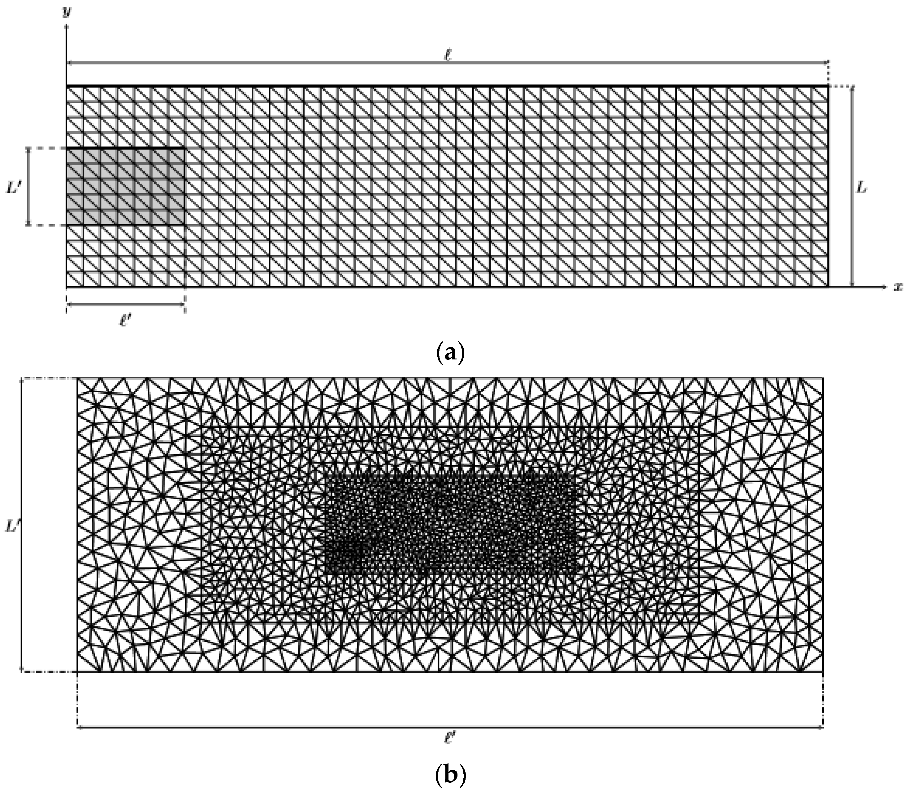
In this contribution, the space discretization is obtained by applying a classical finite element method (FEM) (Galerkin formulation) according to Kolossov et al. [16]. The non-linearity of the material properties is taken into account in a semi-implicit way. However, to obtain a good description of the laser intensity distribution (Equation (4)) at a sub-millimetric scale without exploding the number of nodes needed to mesh the entire domain Ω (with lateral dimensions of some centimeters), local refinements have to be used. The main novelty of this approach is to apply the non-conforming technique developed by Boillat [20]. The fine mesh is the re-union of a coarse tetrahedral mesh and of a much finer prismatic mesh. The coarse mesh (see Figure 3a) is created by subdividing parallelepipedons and the fine mesh (see Figure 3b) is obtained by extruding in the z-direction a triangular mesh of the surface in the xy plane, giving a 3D model.

The fine mesh moves to be always correctly centered with respect to the laser beam location (see Figure 1). Since the two meshes are not conformal, the motion of the fine mesh does not impact the coarse one, which saves a lot of computational effort. No re-meshing is needed. However, this approach has a drawback. The temperature continuity constraint is not implicitly fulfilled and has to be imposed by penalizing the non-continuous FEM shape function according to Boillat [20].

2.4. Laser Setup, Materials and Characterization Methods

In this work, a continuous wave (CW), high-power diode laser LDM 1000 from Laserline GmbH with a 980 nm wavelength was coupled to a fixed focusing head. At the focus point distance of 297 mm, the spot diameter is 0.9 mm with a flat top distribution. The displacement is provided by an x–y table that allows movement in both directions mounted below the process chamber. To avoid oxidation during the process, the chamber is filled with argon. A schematic drawing as well as a picture of the setup is shown in Figure 4.

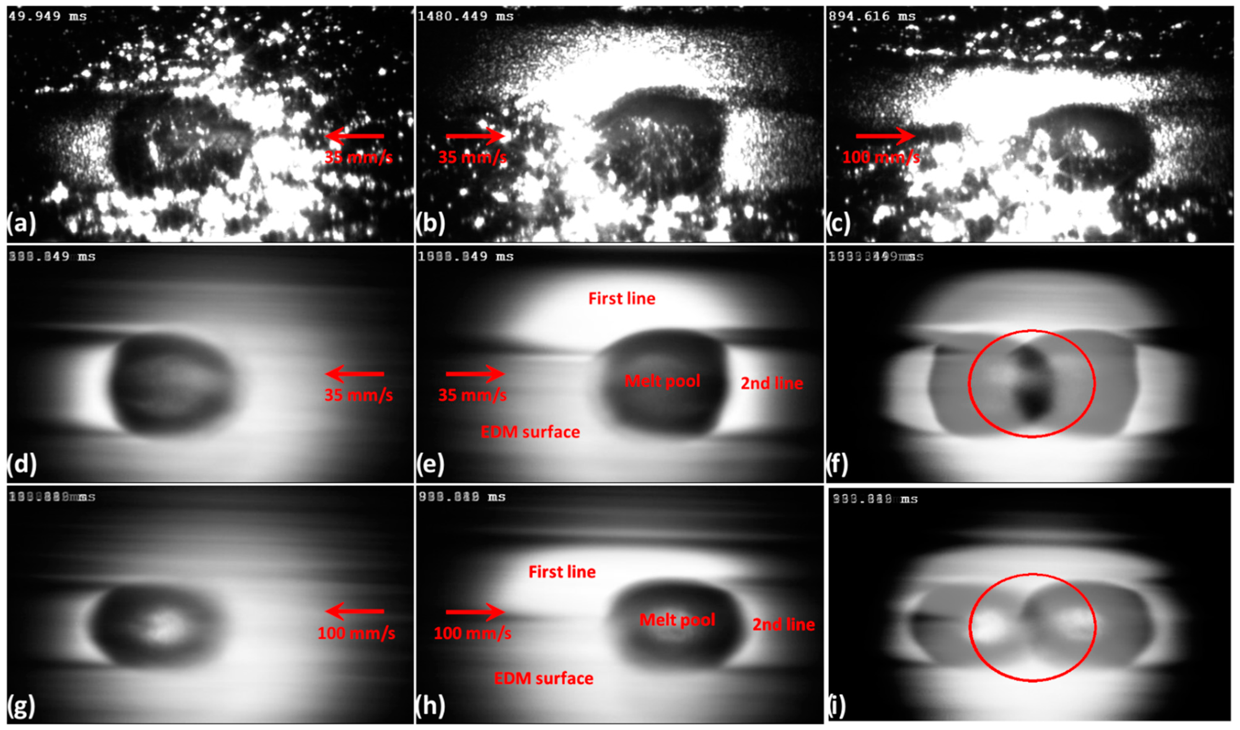
In situ observation of the melt pool was carried out with a Motionpro Y4 high-speed camera from Videal mounted with a Moritex ML-Z07545 telecentric objective. The camera was positioned as shown in Figure 4 and allows observation of the melt pool with a small angle compared to the laser beam. The objective was fitted with low pass filter (cut-off 800 nm) in order to block the back-reflected laser light from entering the camera. Additional light in the visible range was provided by a light fixed on the right-hand side of the setup. In these conditions and taking into account the size of the melt pool observed, the frame rate was 10 kHz.

For static experiments, the laser and the camera were triggered together. The laser power was kept constant at the desired level and was switched off after a given time. The camera kept recording 100 ms afterwards to capture the solidification.

For each moving experiment, the motion of the workpiece was started first in the x-direction. Once the workpiece reached constant speed, the laser and the camera were triggered together. The laser stayed on for a defined displacement. After the laser was stopped, the table was decelerated to a stop. For the case where several lines were observed, the table was moved by a hatching distance in the y-direction. Then, the process could start again in the opposite direction along the x-axis. The process was repeated for the number of lines desired.

The workpieces were made of X38CrMoV5-1 hardened tool steel rectangular plates with dimensions of 70 × 70 × 7 mm³. On the top surface, a region of 50 × 50 mm² was prepared by EDM. The finishing state of the surface was CH30 on the Charmilles scale for EDM which corresponds to a roughness Ra of 3.15 µm. This is also the initial state prior to the LP process.

The total reflection of the steel EDM surface was measured at room temperature with a Lambda 900 spectrometer from Perkin Elmer fitted with an integrating sphere. The absorption is then defined as a = 1 − R, where R is the total reflection (both diffuse and specular).

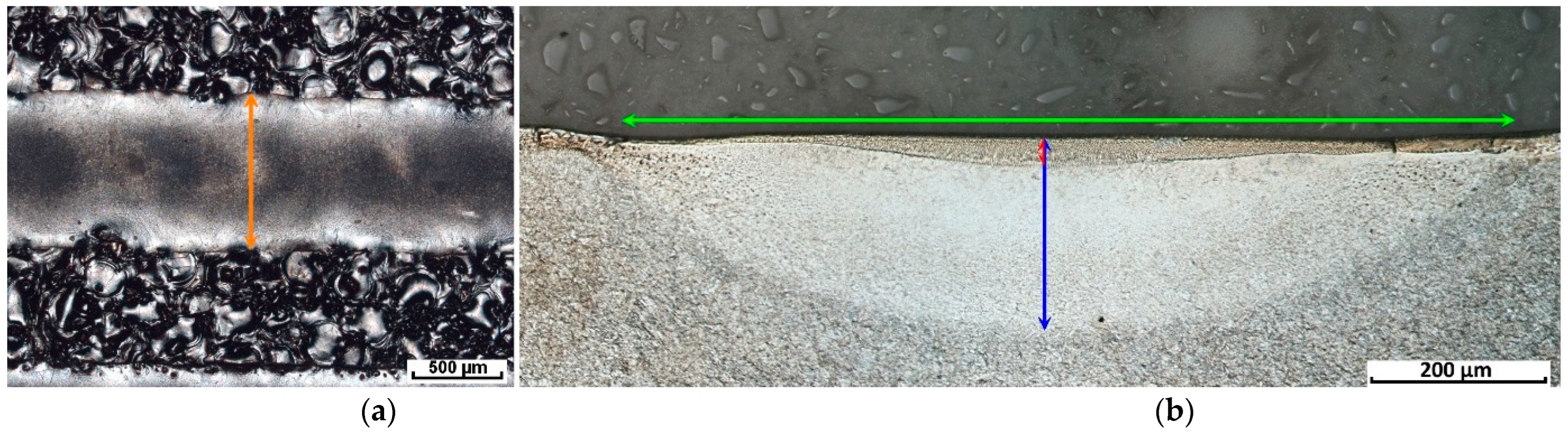
The lines and points produced were observed under an optical microscope to determine the width of the melt pools. The workpieces were then cut in cross sections to observe the size and shape of the re-melted layer and the heat-affected zone (HAZ). The cross sections were ground and polished up to colloidal suspension to obtain a mirror polish. During the next step, they were etched for 20 s with 5% Nital solution and observed with an optical microscope.

3. Results and Discussion

3.1. Static Experiments

The static experiments were designed to study a simplified case of laser polishing. Without displacement, the melt pool is circular and symmetric, and the static conditions are ideal to observe the melting of the surface and the following solidification after the laser power is switched off.

3.1.1. Experimental Results

A typical example of the melting of the surface is illustrated in Figure 5 and the corresponding high-speed movie can be seen at: https://www.empa.ch/web/s204/modellinglaserpolishing1 (accessed on 8 July 2022). In this figure, the evolution for a complete laser illumination (997 ms) at 317 W is shown from left to right and top to bottom. The time indicated in each picture corresponds to the start of the laser irradiation. A few frames were selected from the high-speed images; the complete sequence can be watched in the videos at the link above.

The first frame shows the initial surface just before the start of the laser illumination. The contrast is coming from the reflection of the visible external lightning on the asperities of the rough EDM surface. At the start of the illumination, only minor changes are visible (see green arrows at t = 0 ms) as most of the laser light is filtered out by the low pass filter. After 10 ms of laser illumination, the surface has not changed much. The bright spots in the center appear a little wider and could be a sign of the first melting of the top surface. At 20 ms, the center of the image shows that the bright spots are spreading even more as the melting progresses. After 30 ms, an elliptical melt pool is visible. The ellipse is due to the perspective induced by the angle of the camera. As the time progresses, the melt pool becomes better defined and augments its size (50 to 996.7 ms). Moreover, the center of the melt pool rises in brightness as the time passes. This is due to thermal emissivity of the center of the melt pool as the temperature increases.

The solidification sequence of the same experiment is given in Figure 6, similarly to Figure 5. The corresponding high-speed movie can be seen at: https://www.empa.ch/web/s204/modellinglaserpolishing1 (accessed on 8 July 2022). In this figure, the time stamps refer to the time the laser light was switched off, which was just after the last frame of Figure 5 (996.7 ms). The first frame in Figure 6 corresponds to a time of 0.3 after the laser light was turned off and this corresponds to 0.3 + 996.7 = 997.0 ms from the start of the laser illumination. The first line of images (0.3 to 1.5 ms) shows a clear cooling of the melt pool as the brightness of the center comes rapidly back to dark grey. The brightness settings of the images are the same as in Figure 5 and the cooling is already very high, 0.3 ms after the end of laser illumination, and this is evident when comparing to the last frame of Figure 5 with the first one in Figure 6. After 1.8 ms, the first traces of the solidification are visible (see green arrows at 1.8 ms). It is possible that the solidification of the edge started earlier but it is not visible on the images. After this time, the melt pool in the center decreases in size as the solidification front progresses. Solidification is finished 4 ms after the end of the laser illumination. The re-solidified region appears bright as it reflects lots of light towards the camera. It is also significantly more uniform than the EDM surface visible around the re-melted surface and this shows the positive effect of the polishing process on the surface roughness.

Based on the high-speed images, the evolution of the melt pool with time can be measured and the results are shown in Figure 7. As seen on the frames in Figure 5 and reported in Figure 7, no clear melt pool is visible at 20 ms, whereas at 30 ms the melt pool has already a significant width close to 0.6 mm which is half the final size of the melt pool. Once the melt pool is formed, it expands rapidly afterwards as shown in Figure 5 and Figure 7 (30 to 250 ms). A small increase is still visible until 500 ms when the melt pool reaches a stable width of 1.2 mm. The details of the solidification sequence from Figure 6 are given in the inset of Figure 7. From these figures, at the end of the laser illumination (997 ms), the width of the melt pool decreases almost instantly to zero on the main graph. The solidification is clearly visible after 1.5 ms, from which the size of the melt pool can be precisely measured until it disappears completely at 4 ms, giving a total time (illumination and solidification) of 1’001 ms (1.001 s).

3.1.2. Simulation Results

For all simulations, a domain of 10 × 20 × 2 mm was employed. Figure 8 shows the meshes (coarse and fine) used to guarantee the quality of simulation results. Tests using various absorption coefficients in the liquid were performed. For time discretization, two time steps were employed: one for the heating part (1 ms) and another for the cooling part (0.1 ms). Note that since the values of some physical properties are not well known (in particular emissivity and natural convection coefficient (boundary conditions)), some sensitivity studies were carried out. The obtained results demonstrated a very low influence of the variation of these parameters. In contrast, the thermal conductivity significantly affects the size of the melt pool and its value is not well known in the liquid region. However, the values referenced in Lucefin [17], SIJ Metal Ravne [18], and Matmach [21] and their variation versus temperature are close. So, the value presented in Figure 2 can be considered as a good approximation. The simulation results presented hereafter correspond to a constant parameter set.

As mentioned, the absorption coefficient corresponding to CH30 (representative of the treated workpieces with Ra = 3.15 μm) for solid material was measured with a value of a_s = 35% and so this value was kept constant. In contrast, values of the absorption coefficients in liquid material (a_l) ranging between 20 and 30% were tested. Figure 9 presents the results of the sensitivity analysis obtained for the volume of the melting pool versus time for various absorption coefficients in the liquid region. The differences are important and such results show the necessity to precisely measure or model the absorption coefficient before any simulation.

It is also possible to compute the diameter of the melting pool (x-direction) and the depth of the liquid region. As for the volume, a_s = 35% and a_l values ranged from 20 to 30%. Figure 10 shows the results for such quantities and the differences are less important as compared to the volume (Figure 9). Figure 11 shows the same results as Figure 10 but with a zoom in on the cooling part.

3.1.3. Comparisons of Experimental and Simulation Results

For the experimental results, Figure 7 shows a maximum size of 1.2 mm for the melt pool width. Comparing Figure 7 and Figure 9, it is observed that the simulation that best fits this value was obtained with a constant absorption coefficient equal to 0.35 (a_s = a_l = 0.35). However, we will see below that this curve is probably not the one to consider for the comparison.

In the experimental solution, the melt pool width seems to reach a constant value, which is not the case for the simulation results. However, this effect is less visible when using a smaller absorption coefficient. In Figure 12, a comparison between experimental and simulation results (two different absorptions) for the time evolution of the melt pool during the heating part and during the cooling part are given. From this figure, it is obvious that after 70 ms, the width predicted is significantly lower than the measured one (between 20 and 50% lower). If a comparison is made for the cooling part, it seems evident that the simulation curve that best fits the experimental results corresponds to an absorption of ≈25% in the liquid. An explanation could be that we chose a weakly coupled model and so neglected the influence of the convection in the liquid in the thermal model. This explanation is supported by the fact that effects of “wetting” are observed during the experiment, which prove that convection movements are important. Finally, the precision of the experimental measurement is ±0.1 mm.

Static experiments with relatively long laser illuminating times are more difficult to simulate than regular polishing experiments (moving laser) (see Section 3.2 and Section 3.3). The reason is that the convection effects which are not taken into account in the model become more important in the static context.

The heating and cooling rates are well captured by the model. In other words, the development of the melt pool follows a similar growth as the measured values. The solidification predicted by the model is a little slower (see the slope of curves in the inset of Figure 12), but this is also consistent with a narrower melt pool. Indeed, if the convection is the reason for a larger melt pool, it will also mean that the real melt pool is not as deep as the model. Ex situ observations of the cross section of the workpiece have shown that the depth of the melt pool measured is only 90 µm whereas the modelled depth is ≈117 µm (a difference of ≈25%) for the results with a_l = 25%. It is also known that a flatter melt pool will cool faster than a narrower but deeper melt pool due to an increased surface area.

3.2. Moving Experiment: High-Speed Imaging

A moving experiment is more relevant to LP as it reproduces identical conditions as in the industrial process. During these experiments, the workpiece is moved at a constant speed while the laser is static. This configuration makes for easier tracking of the melt pool as the high-speed camera is also static and centered on the laser position. It produced a similar outcome as a static workpiece with the laser moving at constant speed in the opposite direction.

3.2.1. Experimental Results

Some typical examples of experiments with different velocities and directions are given in Figure 13a–c. The corresponding high-speed movie can be seen at: https://www.empa.ch/web/s204/modellinglaserpolishing1 (accessed on 8 July 2022). They represent values in the range often encountered for LP of rough workpieces. The first line of images is representative only of the first line in real process whereas the return line is representative of the rest of LP where the surface to be treated is scanned with a given overlap between the process lines. In Figure 13a, the melt pool for a first line at 35 mm/s is clearly visible in the center of the image (in dark). It is surrounded by the EDM surface that again consists of a succession of bright and dark regions due to the high roughness of the workpiece. On the left-hand side of the melt pool is the re-solidified line. This line appears much smoother as compared to the EDM surface and again shows the positive polishing effect of the process on the surface roughness. The surface roughness was reduced by a factor between 3 and 5 depending on the process parameters. The melt pool edge is not very well-defined when in contact with the EDM surface and fluctuates due to the variations of the topography. The fluctuations are better seen on the videos of the experiment available at: https://www.empa.ch/web/s204/modellinglaserpolishing1 (accessed on 8 July 2022). For the return line with an overlap of 30% shown in Figure 13b, the fluctuations are reduced for the part of the melt pool that is overlapping with the first line. Finally, Figure 13c shows also a second line of an experiment but at higher velocity (100 mm/s) and higher power (561 W). The increase in laser power is necessary to compensate for the increased velocity so that the maximum temperature of the melt pool stays constant. In Figure 13c, it is observed that the shape of the melt pool becomes oval due to a reduction of the width and a slight increase of the length in the direction of the workpiece movement.

In order to avoid the influence of the fluctuations due to the roughness, averaged images were produced for the different conditions. The average images are simply realized by stacking all steady-state images together and then for each pixel calculating the average intensity of all images. The resulting averaged images are presented in Figure 13d,e,g,h for the first and second lines at 35 and 100 mm/s, respectively. Based on these images, we see that the melt pool is better defined. In Figure 13d,g, the EDM also appears almost as a bright uniform region due to the random positions of the bright spots over the length travelled. For the return lines (Figure 13e,h), the first line is also clearly visible as the brightest region as it is very flat and so reflects most light towards the camera. The melt pools appear mostly as a uniform dark grey and have better defined shapes. Furthermore, the borders of the melt pools positioned over the first lines are very well defined. This shows that the surface of the first line is mostly flat whereas in the overlapping region, no fluctuation of the melt pool size is provoked by the topography variations. On the other hand, over the EDM, the melt pool transitioned from dark grey (the color of the melt pool) to light grey (color of the solid EDM surface). This transition region is where some fluctuations of the melt pool occur due to the fluctuations of the surface topography.

As the camera and laser positions are fixed and did not change during the first line or second line, it is interesting to superpose both pictures to evaluate the position of the melt pool relative to the laser position. The combined image is obtained by superposing the image from the first line with the image of the second line and taking 50% of the pixel intensity of each picture. The resulting images are shown in Figure 13f,i for 35 and 100 mm/s, respectively. The two melt pools form a kind of Venn diagram as they appear darker where they intersect as both melt pools are dark and with a medium shade of grey where only one of the melt pools is present. The solid EDM surface is a light grey all around. Based on these observations, the theoretical position of the laser beam can be positioned at the center of the intersection of the two melt pools (see red ellipses). As can be seen for both melt pools, a large part of the melt pool is trailing the laser spot and is not situated in the laser spot. The melt pool starts only after a third of the spot diameter for 35 mm/s and close to half the diameter at 100 mm/s. The melt pool is also trailing further behind the laser spot as the speed increases.

3.2.2. Simulation Results

Simulations were performed with the same main parameters as those used for the fixed laser case. The velocities of the laser were set to 20, 30, 50 and finally 100 mm/s. The corresponding time steps are: 0.5, 0.28, 0.2, 0.1 ms. The laser powers are identical to those in the experiments. For each case, the whole simulation corresponds to a laser polishing treatment length of approximatively 10 mm. The absorption coefficients used were a_s = 35% and a_l = 30%.

To confirm the predictability of the model, the size, shape and position of the melt pool relative to the laser spot were also simulated for different velocities and power. The results of the evolution of the size and shape for the simulated melt pools at the different velocities and adjusted power are shown in Figure 14. The laser powers were chosen to give approximately the same maximum temperature and this is confirmed by the color coded scale. In these conditions, the melt pool is becoming smaller with an increased velocity and also trails further away from the laser spot. The shape of the melt pool also differs from the observations with the high-speed camera. Indeed, the shape of the melt pool is almost perfectly round at low speed and has an increasing tail as the velocity increases, but maintains a round shape at the front of the melt pool (front on top of each simulation in Figure 14). This is not exactly what was observed in Figure 13, as the shape at low speed is mostly round with a flat tail and almost elliptical at high speed. The reason for these differences is not yet known, and could be due once again to the effect of convection in the liquid.

3.2.3. Comparisons of Experimental and Simulation Results

In

Table 1. Laser parameters, with the melt pool characteristics measured and simulated.

Velocity	Power	Width Melt Pool	Length Melt Pool	Shift Edge
[mm/s]	[W]	[µm]	[µm]	[µm]
20	615	1259	1460	142
20	615	985	1159	−32
35	415	891	922	−252
35	415	760	782	−199
50	454	726	790	−309
50	454	731	158	−239
100	561	588	810	−385
100	561	712	712	−291

, the measured widths and lengths of the melt pool sizes are given in normal font whereas the simulated results are in blue italic font (a line below) for the same laser conditions. The width of the melt pool is measured perpendicularly to the moving direction; the length is measured parallel to the moving direction. The edge shift was also measured in the moving direction and is the difference between the leading edge of the laser spot with the leading edge of the melt pool. It is measured as positive if the melt pool is in front of the laser spot (see first experiment in Table 1), and negative if the melt pool is behind the laser spot.

The first experiment in Table 1 corresponds to exaggerated conditions with low velocity and high power to create extreme conditions to test the model. This condition is not suitable for LP as it will create a too deep melt pool far from the shallow melting desired for LP. The other three conditions are conditions suitable for LP and the laser velocities of 35 and 100 mm/s are the same conditions as in Figure 13. As can be seen, the first condition creates a markedly larger melt pool than the spot size. It is also the only condition where the melt pool is in front of the laser spot. Due to its length, the region trailing the spot size (length − laser diameter − shift edge = 1460 − 900 − 142 = 418 µm) is still bigger than the region in front (142 µm). The other conditions produce a rounder melt pool at low velocity and one which is more elongated at higher velocity. They also all trail the laser spot and the edge shift increases with velocity.

As evident from Table 1, most of the values obtained from the simulations are below the experimental values. The reason could be similar to the static experiment and could come from the absence of the strong coupling with convective flow inside the melt pool. Another explanation could come from the absorption. Indeed, the absorptivity for the EDM surface was measured at room temperature and taken as a constant for the solid (a_s = 35%). It is certainly possible that the absorptivity changes with temperature and/or also with the laser intensity. The absorptivity of the liquid was unknown and must be taken between a_l = 25–30% after fitting with the experimental results.

The static simulations are able to predict both the elongation of the melt pools and the edge shift with velocity. The order of magnitude of the sizes is acceptable and some imprecision on the size measurements are also possible as they are coming from the high-speed imaging where one pixel is approximately 6 µm and observed with an angle.

3.3. Moving Experiment: Microstructure Observation and Adjustment of the Absorption

3.3.1. Microstructure Observations and Adjustment of the Absorption

One of the critical material parameters for simulating laser processes is the light absorption of the given material at the laser wavelength. Indeed, the absorption of light gives the source term in the heat equation and so determines the thermal behavior of the material. For the tool steel used in this study with the EDM rough surface (Ra = 3.15 µm), the absorption was measured at 35%. This value is dependent on the roughness and evidence of this is given by the fact that the absorption was measured at 30% for the same material but with mirror polish finish. This is consistent with the study of Wang et al. [22] who found that an increase of the roughness leads to an increase of the absorption. It is unlikely that a constant absorption is the best solution in simulation since several effects can occur such as Drude absorption [23], oxidation [24], or changes of surface roughness [25].

Schmid et al. [26] demonstrated that the absorption of the liquid tool steel is also unknown due to the complexity of measuring this property. As a consequence, for the simulations, the absorption of the liquid was fitted based on the experimental measurements of the size of the melt pool and HAZ observed during the experiments.

3.3.2. Experimental Results

A typical example of a re-melted line is shown in Figure 15. The width of the melt pool is clearly visible on the top view of Figure 15a, as the re-melted layer is flatter than the original EDM surface situated above and below the line. On the cross section in Figure 15b, three regions are visible. First, at the top of the workpiece, there is the shallow re-melted layer defined in length by the blue arrow and in depth by the red arrow. Below, a well-defined circular area is visible and is delimited by the blue arrow. This region is known as the HAZ, where the temperature was sufficiently high for an austenitization to occur but lower than the melting temperature. Finally, below and on the sides of the HAZ, the bulk microstructure of the hardened tool steel is clearly observable.

3.3.3. Simulation Results

Simulations were performed with the same main parameters as those of the first moving experiment but with various values of absorption coefficients in the liquid (a_l). The laser power was 401 W and the workpiece velocity was 35 mm/s. The obtained solutions are visualized at time 0.5 s. At this time, the process can be considered in a steady state. Figure 16 shows the result of the simulations obtained for absorption values between 0.20 to 0.35 in the molten region. The melting pool shown in the figure corresponds to an iso-volume for a temperature higher than 1’505 °C. Not only are the sizes of the liquid zones different, but also the shapes. Note that some artefacts due to the meshes are visible in Figure 16.

The same graphs can be obtained from the HAZ zone considering an iso-volume with a temperature higher than the austenitization temperature of 950 °C.

3.3.4. Comparisons of Experimental and Simulation Results

The first simulation was performed with a constant absorption coefficient equal to 0.35. Figure 17 shows the melting pool and the HAZ (top), and their corresponding bounding boxes (bottom). The reason for using bounding boxes instead of the isotherm line corresponding to the liquidus temperature (1’505 °C) and the austenitization temperature (950 °C) is due to the fact that the experimental results are measured after the laser treatment, whereas the areas of interest in the numerical simulation are computed during the treatment. In other words, during the simulation, the deeper part of these two regions does not necessarily correspond to their widest part. As it can be seen in Figure 17, the sizes of the melting pool and HAZ are largely over-estimated.

The absorption coefficient of the liquid was then decreased in order to obtain a solution closer to the experimental results. A good solution was found for a liquid absorption coefficient of 0.25 and is presented in Figure 18. In this case, the size of the melting pool better fits the experimental result.

With this liquid absorption, the size of the melt pool fits better to the experimental result. The size of the HAZ is still slightly exaggerated. This, however, can be explained, as the austenitization temperature is from the phase diagram where the phases are given without taking into account the kinetics of the reaction. In this present case, the heating by the laser and subsequent cooling only last for a fraction of a second. It is probable that in these conditions, a quite high overheating is needed to provide the driving force for the phase transformation to occur. From the simulations it appears that in these conditions, the austenitization occurs only above 1’100–1’200 °C.

A drop in the absorption as the material melts was also reported by Simonds et al. [25] during conduction welding. The explanation for a decrease of the absorption is the decrease of the roughness of the metal in the liquid state.

Finally, based on the results presented in this paper, we can conclude that the thermal model is sufficiently accurate to model the depth and size of the melt pool. It provides a useful tool to estimate the changes on the melt pool when the laser parameters (velocity or power) are varied. In a second part of our research, a flow model will be developed and solved inside the melt regions modelled with the current approach, as illustrated in Figure 19. A weak coupling is used between the thermal solution and a computational fluid dynamics (CFD) calculation.

4. Conclusions

A thermal model based on the Chernoff formula was developed and compared to experimental data for the laser polishing of rough tool steel. The main properties missing from the model were the light absorption coefficient evolution with the temperature especially in the liquid state of the steel. The best results are obtained with two constant coefficients; one for the solid based on the measurement at room temperature (a_s = 35%) and one for the liquid fixed so that the model fits the experiment data (a_l = 25%). A lower value can be explained by the smoother surface of the steel in the liquid state as compared to the rough solid.

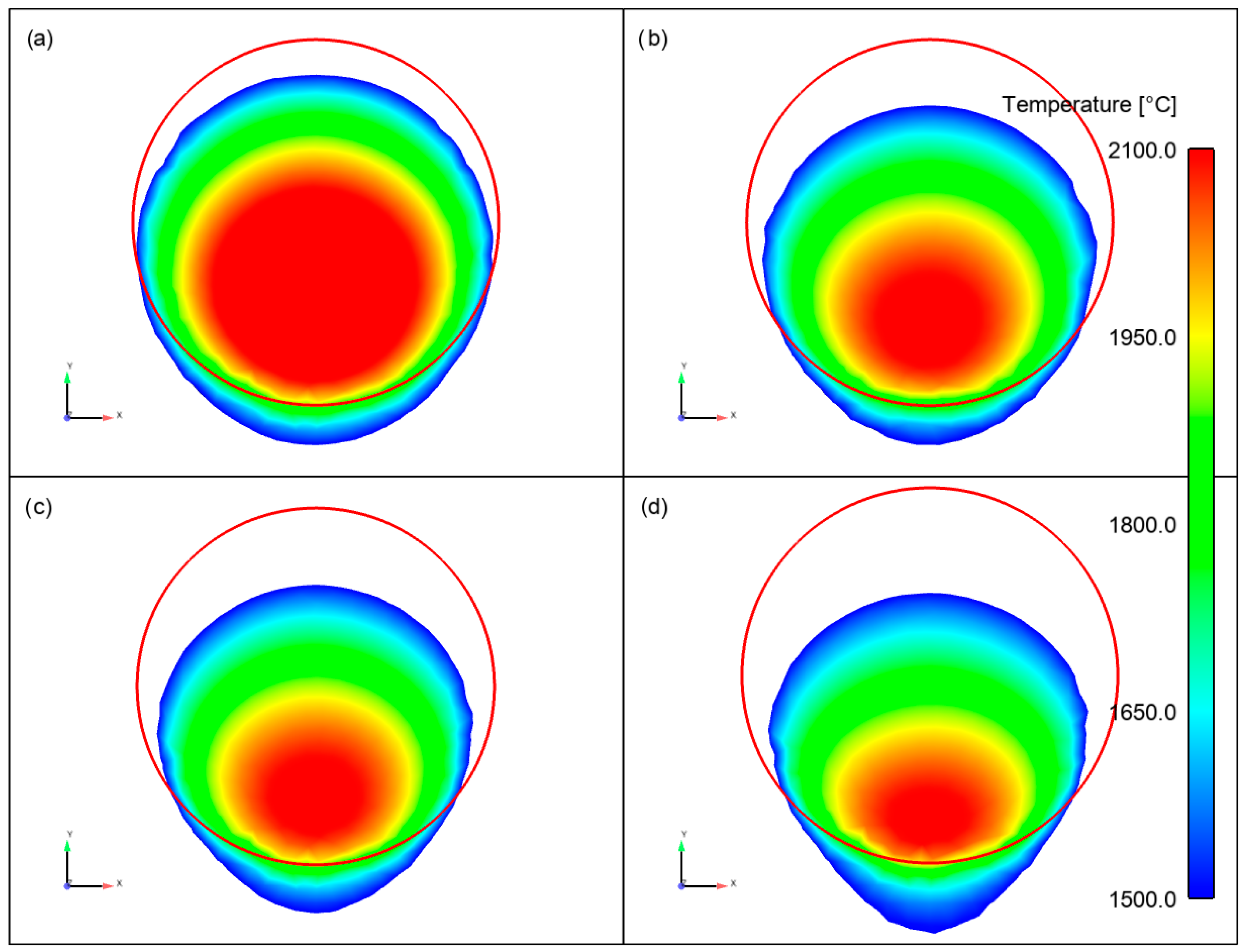
The model was first tested with some static experiments with the laser spot not moving and a long illumination time of close to 1 s. In these conditions, the model shows some limitations due to the lack of coupling between the convection and thermal model. The experimental melt pool is wider and shallower than the simulated melt pool. The volume of the liquid is well simulated with a liquid coefficient of absorption of 0.25. Due to the shallower melt pool and increased surface of the experimental melt pool the solidification time of the experiment is also shorter.

The limitation of the model not taking account of the convection in the thermal model is less important in the real process with a moving laser beam as the interaction time is decreased. The model can estimate the elongation of the melt pool with increasing speed and the trailing of the melt pool with regard to the laser spot. The volume is also relatively well simulated with an absorption of 0.25 in the liquid state. As for the static experiment, the experimental melt pools have a slightly larger surface but a shallower depth than the simulated melt pools. Again, this can be explained by the lack of coupling between convection and thermal models in the simulation.

Finally, the results show that the model is able to represent the thermal behavior of the tool steel during laser polishing. The melt pool is relatively well estimated and we are confident that the thermal fields simulated are close to the reality. In the next study, a flow model will be applied in the simulated melt pool to observe the effect of laser polishing on the surface roughness.

References

1. Emmler, A.; Willenborg, E.; Wissenbach, K. Laser Polishing. In Proceedings of the Laser Applications in Microelectronic and Optoelectronic Manufacturing (LAMOM) XVII, San Francisco, CA, USA, 21–26 January 2012; p. 82430W. [Google Scholar]
2. Shirk, M.D.; Molian, P.A.; Malshe, A.P. Ultrashort pulsed laser ablation of diamond. J. Laser Appl. 1998, 10, 64–70. [Google Scholar] [CrossRef]
3. Pimenov, S.; Kononenko, V.; Ralchenko, V.; Konov, V.; Gloor, S.; Lüthy, W.; Weber, H.; Khomich, A. Laser polishing of diamond plates. Appl. Phys. A 1999, 69, 81–88. [Google Scholar] [CrossRef]
4. Ukar, E.; Lamikiz, A.; de Lacalle, L.N.L.; del Pozo, D.; Arana, J. Laser polishing of tool steel with CO2 laser and high-power diode laser. Int. J. Mach. Tools Manuf. 2010, 50, 115–125. [Google Scholar] [CrossRef]
5. Yung, K.; Wang, W.; Xiao, T.; Choy, H.; Mo, X.; Zhang, S.; Cai, Z. Laser polishing of additive manufactured CoCr components for controlling their wettability characteristics. Surf. Coat. Technol. 2018, 351, 89–98. [Google Scholar] [CrossRef]
6. Richter, B.; Blanke, N.; Werner, C.; Vollertsen, F.; Pfefferkorn, F.E. Effect of Initial Surface Features on Laser Polishing of Co-Cr-Mo Alloy Made by Powder-Bed Fusion. JOM 2019, 71, 912–919. [Google Scholar] [CrossRef]
7. Obeidi, M.A.; McCarthy, E.; O’Connell, B.; Ahad, I.U.; Brabazon, D. Laser Polishing of Additive Manufactured 316L Stainless Steel Synthesized by Selective Laser Melting. Materials 2019, 12, 991. [Google Scholar] [CrossRef] [PubMed] [Green Version]
8. Ramos-Grez, J.A.; Bourell, D.L. Reducing surface roughness of metallic freeform-fabricated parts using non-tactile finishing methods. Int. J. Mater. Prod. Technol. 2004, 21, 297–316. [Google Scholar] [CrossRef]
9. Shao, T.; Hua, M.; Tam, H.Y.; Cheung, E.H. An approach to modelling of laser polishing of metals. Surf. Coat. Technol. 2005, 197, 77–84. [Google Scholar] [CrossRef]
10. Nüsser, C.; Kumstel, J.; Kiedrowski, T.; Diatlov, A.; Willenborg, E. Process- and Material-Induced Surface Structures During Laser Polishing. Adv. Eng. Mater. 2015, 17, 268–277. [Google Scholar] [CrossRef]
11. Perry, T.L.; Werschmoeller, D.; Li, X.; Pfefferkorn, F.E.; Duffie, N.A. Pulsed laser polishing of micro-milled Ti6Al4V samples. J. Manuf. Process. 2009, 11, 74–81. [Google Scholar] [CrossRef]
12. Ramos, J.A.; Bourell, D.L. Modeling of surface roughness enhancement of indirect-SLS metal parts by laser surface polishing. In Proceedings of the TMS Fall Meeting, Seattle, WA, USA, 17–21 February 2002; pp. 191–202. [Google Scholar] [CrossRef]
13. Zhang, J.-J.; Zaho, L.; Rosenkranz, A.; Song, C.-W.; Yan, Y.-D.; Sun, T. Nanosecond pulsed laser ablation on stainless steel−combining finite element modeling and experimental work. Adv. Eng. Mater. 2019, 21, 1900193. [Google Scholar] [CrossRef]
14. Zhang, J.-J.; Zhao, L.; Rosenkranz, A.; Song, C.; Yan, Y.; Sun, T. Nanosecond pulsed laser ablation of silicon—finite element simulation and experimental validation. J. Micromechan. Microeng. 2019, 29, 075009. [Google Scholar] [CrossRef]
15. Mohajerani, S.; Bordatchev, E.V.; Tutunea-Fatan, O.R. Recent Developments in Modeling of Laser Polishing of Metallic Materials. Lasers Manuf. Mater. Process. 2018, 5, 395–429. [Google Scholar] [CrossRef]
16. Kolossov, S.; Boillat, E.; Glardon, R.; Fischer, P.; Locher, M. 3D FE simulation for temperature evolution in the selective laser sintering process. Int. J. Mach. Tools Manuf. 2004, 44, 117–123. [Google Scholar] [CrossRef]
17. Lucefin, S.P.A. Reference for X38CrMoV5-3 Alloy. Available online: https://www.lucefin.com/wp-content/files_mf/15294144241.2367X38CrMoV53.pdf (accessed on 9 July 2022).
18. SIJ Metal Ravne. Reference for X38CrMoV5-3 Alloy. Available online: https://steelselector.sij.si/steels/UTOPMO7.html (accessed on 10 April 2022).
19. Magenes, E.; Nochetto, R.H.; Verdi, C. Energy error estimates for a linear scheme to approximate nonlinear parabolic problems. ESAIM Math. Model. Numer. Anal. 1987, 21, 655–678. [Google Scholar] [CrossRef] [Green Version]
20. Boillat, E. Finite element methods on non-conforming grids by penalizing the matching constraint. ESAIM Math. Model. Numer. Anal. 2003, 37, 357–372. [Google Scholar] [CrossRef] [Green Version]
21. Matmatch. Reference for X38CrMoV5 Alloy. Available online: https://matmatch.com/materials/minfc5954-iso-4957-grade-x38crmov5-1-soft-annealed-a- (accessed on 9 July 2022).
22. Wang, J.-T.; Weng, C.-I.; Chang, J.-G.; Hwang, C.-C. The influence of temperature and surface conditions on surface absorptivity in laser surface treatment. J. Appl. Phys. 2000, 87, 3245–3253. [Google Scholar] [CrossRef] [Green Version]
23. Arnold, G.S. Absorptivity of several metals at 106 μm: Empirical expressions for the temperature dependence computed from Drude theory. Appl. Opt. 1984, 23, 1434–1436. [Google Scholar] [CrossRef]
24. Kwon, H.; Baek, W.-K.; Kim, M.-S.; Shin, W.-S.; Yoh, J.J. Temperature-dependent absorptance of painted aluminum, stainless steel 304, and titanium for 1.07 μm and 10.6 μm laser beams. Opt. Lasers Eng. 2012, 50, 114–121. [Google Scholar] [CrossRef]
25. Simonds, B.J.; Sowards, J.W.; Hadler, J.; Pfeif, E.; Wilthan, B.; Tanner, J.; Harris, C.; Williams, P.A.; Lehman, J. Dynamic and absolute measurements of laser coupling efficiency during laser spot welds. Procedia CIRP 2018, 74, 632–635. [Google Scholar] [CrossRef]
26. Schmid, M.; Zehnder, S.; Schwaller, P.; Neuenschwander, B.; Held, M.; Hunziker, U.; Zuercher, J. Measuring optical properties on rough and liquid metal surfaces. Proc. ALT12 2012, 1. [Google Scholar] [CrossRef]
Figure 1. The simulated part (domain Ω ) and its dimensions (dashed zone: laser spot).
Applsci 12 08409 g001
Figure 2. Temperature T (continuous. line) and thermal conductivity k (dashed line) as a function of the specific enthalpy for the X38CrMVo5-1 steel. This figure has been constructed based on information found in the literature, in particular Lucefin [17]).
Applsci 12 08409 g002
Figure 3. (a) Coarse mesh in the xy plane and the possible position of the fine mesh in gray and (b) Fine mesh in the xy plane and a representative coarse cell (in gray).
Applsci 12 08409 g003
Figure 4. (a) Schematic representation of the experimental setup of LP; (b) photography of the actual setup.
Applsci 12 08409 g004
Figure 5. Evolution of the melt pool during a static experiment, with a power of 317 W for a duration of 997 ms.
Applsci 12 08409 g005
Figure 6. Solidification sequence for the same experiment as in Figure 2. Time stamps are from the end of laser illumination.
Applsci 12 08409 g006
Figure 7. Evolution of the melt pool with time. Blue diamonds are the measured data from the high-speed images. The inset shows the detail of the solidification.
Applsci 12 08409 g007
Figure 8. Top and side views (transversal cut) of the meshes used for simulations (coarse and fine (right), coarse (center), fine (left)).
Applsci 12 08409 g008
Figure 9. Liquid volume evolution for various absorption coefficients during heating. The inset shows the detail of the cooling.
Applsci 12 08409 g009
Figure 10. Melting pool diameter and depth evolution for various absorption coefficients.
Applsci 12 08409 g010
Figure 11. Melting pool diameter and depth evolution for various absorption coefficients (zoom in the cooling part).
Applsci 12 08409 g011
Figure 12. Time evolution of the melt pool width. The inset shows the detail of the solidification.
Applsci 12 08409 g012
Figure 13. (a) First line at 35 mm/s and 415 W in the steady state regime. (b) Second line with an overlap of 30% also at 35 mm/s and 415 W also in the steady state. (c) Second line at 100 mm/s and 561 W in the steady state. (d) Average of the light intensity of all images in the steady state for the first line at 35 mm/s and 415 W. (e) Average of the light intensity of all images in the steady state for the second line at 35 mm/s and 415 W. (f) Combination of 50% (d) and 50% (e). (g) Average of the light intensity of all images in the steady state for the first line at 100 mm/s and 561 W. (h) Average of the light intensity of all images in the steady state for the second line at 100 mm/s and 561 W. (i) Combination of 50% (g) and 50% (h). For a scale indication, the ellipses in (f,i) represent the spot diameter of 0.9 mm and so main axes give the scale in x and y directions. All images have the same scale.
Applsci 12 08409 g013
Figure 14. Simulation of the melt pool temperature and shape and relative position to the laser beam (red line) for (a) 20 mm/s and 401 W, (b) 35 mm/s and 415 W, (c) 50 mm/s and 454 W and (d) 100 mm/s and 561 W.
Applsci 12 08409 g014
Figure 15. (a) Top view micrograph of a laser re-melted line at 35 mm/s and 401 W (orange arrow shows the width of the re-melted layer), (b) cross section parallel to the orange arrow of the same line as in (a). The re-meted layer is indicated by the red arrow, the HAZ is indicated by the blue arrow (depth) and green arrow (width).
Applsci 12 08409 g015
Figure 16. Melt pool viewed form the top and from the side (perpendicular to the laser direction). (a) For a constant absorption of as = al = 35%, (b) for as = 35% and al = 20%, (c) for as = 35% and as = 25%, and (d) for as = 35% and al = 30%).
Applsci 12 08409 g016
Figure 17. Melting pool (blue) and HAZ (red) with al = 35%. Top: top and side view of the iso-volumes. Bottom: bounding boxes overlaid on experimental results.
Applsci 12 08409 g017
Figure 18. Melting pool (blue) and HAZ (red) with al = 25%. Top: top and side view of the iso-volumes. Bottom: bounding boxes overlaid on experimental results.
Applsci 12 08409 g018
Figure 19. (a) Example of the temperature field simulated for LP of tool steel (complete domain), (b) zoom on the fine mesh region, (c) 3D representation of the melt pool only with temperature.
Applsci 12 08409 g019