Article

A Mixing Process Influenced by Wall Jet-Induced Shock Waves in Supersonic Flow

1
Science and Technology on Scramjet Laboratory, National University of Defense Technology, Changsha 410073, China
2
Department of Aerospace Science and Technology, Space Engineering University, Beijing 101416, China
*
Author to whom correspondence should be addressed.
Appl. Sci. 2022, 12(16), 8384; https://doi.org/10.3390/app12168384
Submission received: 12 July 2022 / Revised: 14 August 2022 / Accepted: 18 August 2022 / Published: 22 August 2022

Abstract

:

Featured Application

The present proposed mixing enhancement strategy can be a good candidate for application in Scramjet and RBCC combustors of hypersonic propulsion systems.

Abstract

With the development of hypersonic air-breathing propulsion systems, such as the supersonic combustion ramjet (Scramjet) and rocket-based combined cycle (RBCC) engines, the mixing process of supersonic airstream with fuel in the engine combustor has been drawing more and more attention. Due to the compressibility effects, the mixing process in a supersonic condition is significantly inhibited. In the present paper, the novel strategy of wall-jet induced shock waves (WJISW) is put forward to realize mixing enhancement. The interaction process between WJISW and the supersonic mixing layer is researched and the enhanced-mixing mechanism is revealed, employing large eddy simulation (LES) methods. The fine vortex structures of the flow field are well captured and presented, utilizing the numerical schlieren technique. Detailed visualization results indicate that WJISW in a low frequency condition can result in the ‘region action mode’ (RAM) never reported before. The drastic dynamic behaviors including growth, deformation, and distortion in the interaction region can undoubtedly promote the mixing of upper and lower streams. The Reynolds stress distributions along the streamwise x-direction suggest that more intense fluctuations can be achieved with a low frequency WJISW. Moreover, a sharp increase in mixing layer thickness can be realized in the interaction region. The dynamic mode decomposition (DMD) analysis results show that the mixing layer evolution process is dominated by the mode induced by WJISW, which leads to the coexistence of both large- and small-scale structures in the flow field. The entrainment process corresponding to large-scale vortices and the nibbling process corresponding to small-scale vortices can obviously promote mixing enhancement. It is suggested that the present proposed strategy is a good candidate for enhanced-mixing with application to Scramjet and RBCC combustors.

1. Introduction

In recent years, with the rise of research on rocket based combined cycle (RBCC) engines and scramjet, efficient mixing of air and fuel under high-speed compressible conditions has become a hot issue. For example, in the current popular RBCC combustion chamber, rich fuel and air mix and diffuse in the flow channel, and sufficient mixing is of great importance to improve engine combustor performance. Whereas, under the limited size of the combustor, the residence time of supersonic flow in the chamber is on the order of milliseconds [1], and this time provided for the mixing of fuel and air is extremely short. Apart from that, although in a low-speed condition the diffusion process of the mixing layer is very fast, the existence of a compressible effect significantly inhibits the growth process of the mixed layer under supersonic conditions. Therefore, considering the limited mixing time and the influence of a compression effect [2,3,4], it is urgent to adopt mixing enhancement strategies to improve mixing efficiency.
In order to realize mixing enhancement of supersonic flow, researchers worldwide have put forward a variety of mixing enhancement techniques, which can be divided into passive active methods. The passive mixing method perturbs the mixing layer by changing the configuration of the middle partition plate of the mixing layer or adding a disturbance device to speed up the mixing. Our previous work comprehensively reviewed passive strategies proposed by investigators to promote mixing [5]. Typical passive mixing enhancement measures include: lobe mixer [6], slope device [7], cavity [8,9], strut [10], and so on. A fact that cannot be ignored is that due to the introduction of a passive device, the inherent defect, including non-ignorable flow loss [11], limits the wide usage of these techniques. Active mixing enhancement methods are to t external energy into the mixing layer by introducing external excitation, and mixing enhancement is achieved by the regulation of the mixing layer. Typical active mixing enhancement strategies include acoustic excitation [12], plasma magnetic fluid excitation [13], blowing and suction [14], reflux device [15], vibration device [16,17], etc. The work conducted by Suzuki [18] et al. indicated that in the low-speed shear layer, sinusoidal excitation can promote earlier instability of the flow, and the rolled-up K–H structures can notably increase the mixing level. Whereas, in supersonic conditions, the effect of an electromagnetic flap is negligible.
Therefore, it can be concluded that the defect of both active and passive strategies calls for newer methods to realize mixing enhancement. It is worth noting that as the inherent flow structures in the confined supersonic mixing layer flow, shock waves [19] and their dynamic behaviors can significantly influence the flow evolution process. Specifically, the interaction between shock waves induced by a wedge shock generator and the mixing layer can notably affect the K–H vortex development. Menon [20] obtained the first experimental visualization results and found that shock wave induced by a wedge generator contributed to mixing enhancement. Lu and Wu [21] used direct numerical simulation (DNS) to research the effect of shock waves on the mixing layer and found that the influence of a shock wave on the mixing layer is very local and the installation should be set as early in the upstream as possible to short the initial mixing distance. Shau [22] claimed that the growth rate of the mixing layer increased slightly under the impingement of shock, but it returned to the original value within a short distance downstream. Gènin and Menon [23] develop a hybrid computation methodology to investigate turbulent flows containing shock waves, concluding that shock can promote high-level mixing in the non-similar region by amplifying the local turbulence, but this trend is limited in local space.
It can be found that a shock wave can achieve mixing enhancement, but with the introduction of a wedge generator, the promoted area is mainly near the interaction point. It is worth noting that as the most typical and simple means of fuel injection, a wall transverse jet and its flow field structure [24,25] and noise control [26] have been studied in detail by many scholars. Due to the jet’s obstruction of the incoming flow, a bow shock wave will be formed in the upstream area of the jet. In addition, because the position of the jet hole is controllable, the position of the shock wave generated by the jet is also controllable, which provides a good idea for us to use the controllable shock wave induced by the jet to achieve mixing enhancement. The previous research [27,28] related to wall jets is limited to the wall jet injecting fuel, whereas our research attempts to use the wall jet to induce a shock wave to act on the plane mixing layer. Based on this, we propose a new strategy called: wall-jet induced shock wave, which retains the advantages of shocks to enhance the growth rate of the downstream mixing layer and overcomes the disadvantage of the local range of shock interaction. Meanwhile, introducing shock waves through the wall-jet can conquer the drawbacks of the passive method and it does not require the participation of fixed devices in the flow field, which reduces flow loss. Furthermore, this scheme holds the advantage of an active method and the position of the shock wave interacting on the mixing layer can be controlled. By introducing shock wave induced through controlled wall jet to promote the mixing enhancement of supersonic mixing layers, it can expand the application of the classical problem of Shock wave/mixing layer interaction (SWMLI) and provide a new method to support the realization of efficient mixing under supersonic conditions.
In the present work, the large eddy simulation (LES) method is employed to analyze the effect of shock waves induced by a wall jet on the supersonic planar mixing layer, and the flow and growth properties of the mixing layer is studied by means of turbulence characteristics and evaluation of the thickness of the mixing layer. Besides, the modal decomposition is performed by the DMD method to further explore the deep-seated mechanism of mixing enhancement influenced by a wall jet. Through extensive reading of the literature, we found that DMD has been applied to the decomposition of the flow field where the moving shock wave [29] is located, which shows the feasibility of DMD. The remainder of this paper is organized as follows: Section 2 gives a brief introduction to the numerical method and the DMD process. Section 3 shows the simulation results in terms of flow field visualization and growth characteristics and analyzes the flow mechanism by mode decomposition. Finally, Section 4 gives the conclusions.

2. Methodology Details

2.1. Governing Equations and Numerical Methods

LES was conducted to solve the flow process by filtering the turbulent motion and decomposing the turbulent flow into large scale pulsations and small-scale pulsations. The large-scale pulsations are solved by direct numerical simulation (DNS) and the mass, momentum, and energy transport of the small-scale pulsations on the large-scale motion are modeled to close the equations, where the model is called a subgrid model. The Navier–Stokes equations, filtered by Deardroff box filtering [30], are as follows:
ρ ¯ t + x i ρ ¯ u ˜ i = 0
t ρ ¯ u ˜ i + x j ρ ¯ u ˜ i u ˜ j + p ¯ δ i j τ ˜ i j + τ i j s g s = 0
ρ ¯ E ˜ t + x i ρ ¯ E ˜ + p ¯ u ˜ i + q ¯ i u ˜ j τ ˜ i j + H i s g s + σ i s g s = 0  
In the above equations, the mark ‘¯’ denotes spatial filtering and ‘~’ denotes Favre filtering. Superscript ‘sgs’ is variances associated with subgrid model. Here, τ i j is the viscous stress tensor, q i is heat flux vector, and δ i j is unit tensor. E is energy, H i is the enthalpy flux vector, and σ i is the energy flux vector.
The kinetic-energy transport sub-grid model is adopted to measure the influence of small-scale transport on large-scale pulsation. The sub-grid viscosity coefficient is defined as
μ t = C k ρ k s g s 1 / 2 Δ f
The subgrid viscous stress tensor meets the equation as following:
τ i j 2 3 ρ k s g s δ i j = 2 C k ρ k s g s 1 / 2 Δ f S ¯ i j
In this equation,
k s g s = 1 2 u K 2 ¯ u ¯ k 2
Δ f V 1 / 3
V is the volume of the grid. Moreover, subgrid kinetic energy can be obtained by the following equation:
ρ k ¯ sgs   t + u ¯ j k sgs   ¯ x j = τ i j u ¯ i x j C ε ρ k s g s 3 / 2 Δ f + x j μ t σ k k sgs   x j
It should be noted that C k , C ε and σ k are constants in above formula. In present work, the implicit method based on density is applied to numerical simulation. The filter equation is discretized by finite volume method and a second-order upwind scheme is utilized to calculate the convection terms. Besides, a second-order central difference scheme is applied to calculating the viscous term, and a second-order implicit scheme is employed to discretize the time. Such numerical schemes [17] are widely used in previous studies on mixing layers.

2.2. Computational Model and Boundary Conditions

As a preliminary work concerning the proposed strategy and relevant enhanced-mixing mechanisms, the two-dimensional compressible N–S equations are solved. The two-dimensional simulation strategy is acceptable in the present study since the computational model is based on the inner flow of a scramjet engine, and a great deal of research with two-dimensional models has already been performed to reveal the relevant flow mechanisms in inner engine flows [31,32]. Moreover, the compressibility effects on mean velocity field and turbulent statistics are researched, employing the two-dimensional method since it is the first step towards understanding the realistic three-dimensional flow, which is much more complex.
The simulation in this paper is based on the model of Yee [33], where the length of the computational domain is 200 mm and the width is 40 mm, corresponding to the height of the inlet on both the upper and the lower sides is 20 mm. The low-speed inlet on the lower side is defined as inlet 1 and the high-speed inlet on the upper side is defined as inlet 2, as shown Figure 1. To enhance the mixing effect of the incoming flow and to simulate the random disturbance of the actual combustor, white noise disturbance is added to both the upstream and the downstream incoming flows. Unlike the previous approach of generating a shock wave through a wedge shock generator, a wall jet (16 < x < 17) at the upper boundary is used in the present work to generate a controllable shock wave with a jet nozzle, and the throat width is 1 mm.
The incoming flow parameters for this calculation are listed in Table 1.
The convective Mach number is defined as
M c = u 1 u 2 a 1 + a 2
and the subscripts 1 and 2 represent the lower and the upper layers of the flow field, respectively. The local sound velocity can be obtained from the relation:
a = γ R T
As for the selection of the boundary condition, the pressure inlet condition is set in the inlet, outlet, and jet nozzle; the slip wall is applied to upper and lower wall. The jet nozzle is set just for the choked state, which is marked by the superscript ‘*’, and the nozzle flow will reach the maximum at this state. The choked flow calculation formula is as follows.
p p 0 = 0.528
p and p 0 are the static and the total pressure of the choked flow, respectively. The total pressure of the jet nozzle is set to fluctuate in the form of a sine curve around 0.02 times the total pressure of the upper incoming flow.
p 0 = p 02   A sin 2 π f t + ζ
p 02 is the total pressure of the upper incoming flow. Here, we set A = 0.01 and ζ = 0.02, and f takes different values in different cases to control the frequency of the jet. This paper sets a case of a mixing layer and two cases of jet shock interference, where f is taken as 2 f 0 and 0.2 f 0 , respectively, and f 0 is the characteristic frequency of an unstable mode of the free mixing layer, the value of which is 3 × 10 4 Hz. The frequencies of different jet shock waves are shown in Table 2.
Because we focus on the interaction of shock wave and mixing layer, the grid is only densified in the the mixing area, and the grid of another area is evenly distributed, which can be seen in Figure 2. Furthermore, the boundary condition does not influence the effect of the shock wave on the mixing layer, so the upper and lower boundaries of the computational domain are set as a slip wall. The advantage of this slip condition over a non-slip condition is that the slip condition demands fewer grids at the boundary, and the shock wave is not smeared in the lower grid resolution. This method is used by many scholars in similar research [34].
In the present work, three sets of grids are used for numerical calculations to verify grid independence, and the number of grids is 1000 × 300, 2000 × 300 and 2500 × 300, respectively. The grids are uniformly distributed in the streamwise x-direction and the transverse grids are refined in the core area. Figure 3 compares the distribution of the mean Mach number along the stream direction at the centerline of the flow field under different grid conditions. It can be found that the value of the time-averaged Mach number along the streamwise direction at the centerline of the flow field under the grid conditions of 2000 × 300 and 2500 × 300 is approximately the same, while it is significantly underestimated under the poor grid condition (1000 × 300) between 0.05 m and 0.07 m in the streamwise x-direction. In order to economize on computational resources, a grid condition of 2000 × 300 is employed for calculation in this paper.

2.3. Code Validations

In order to verify the correctness of the numerical method used in this calculation, the velocity profiles at different streamwise locations are compared between the calculations in this paper and the Geobel–Dutton [35] experimental results, with all conditions consistent. The schematic diagram of the experimental device of a is shown in Figure 4.
The incoming flow conditions of the Geobel–Dutton experimental are listed in Table 3.
Figure 5 gives the comparison between the calculated and experimental velocity profiles at x = 50 mm, x = 150 mm, and x = 200 mm, respectively: H is the distance between the upper and lower boundaries of the flow field, and y 0 is the coordinate value of the centerline of the mixing layer; and U 2 represents the time-averaged velocity value of the high-speed side, and U 1 represents time-averaged velocity value of the low-speed side. Furthermore, we estimated the absolute error of the edge of the mixing layer with the most severe shear, which is 0.035, 0.061, and 0.018 at the streamwise direction of 50 mm, 150 mm, and 200 mm, respectively. The results demonstrate that the LES model used in our research can capture the velocity distribution characteristics of the flow field to a large extent, and the error is small, which proves that the algorithm of this paper is feasible.
Besides, we employed the method used by Smirnov et al. [36] to evaluate the error accumulation of numerical simulation, which is related to grid resolution and physical time. The results are shown in Table 4. As shown in the table, the higher the reliability, the smaller the error. We can conclude that the grid distribution and the numerical procedures can provide high reliability for the research.
Furthermore, we adopt the method used by Celic et al. [37] to estimate the discretization error in CFD calculation and the detailed description of this method can be found in Ref. [37]. Table 5 illustrates the calculation procedure for selected grids: N1, N2, and N3 respectively represent the amount of the three sets of selected grids; r 21 is the ratio of the average length of the second sets of grids to the average length of the first set of grids, and r 32 is the ratio of the average length of the third sets of grids to the average length of the second set of grids; ϕ 1 , ϕ 2 , and ϕ 3 respectively represent the statistical velocity magnitude of the reference location, and the reference location is chosen at (100 mm, 20 mm) at the flow field of the three sets of selected grids; and P, e a 21 and G C I f i n e 21 are the key parameters for the error estimate, and the detailed calculation process can be found in Ref [37]. According to Table 1, the numerical uncertainty in the medium-grid solution for the velocity magnitude should be reported as 0.12%, which meets the demand of CFD.

2.4. DMD Method

The DMD method put forward by Rowley [38] can extract valuable information from the flow field snapshots obtained from computation or experimentation. The snapshot sequence is represented by the matrix V 0 N .
V 0 N = v 0 , v 1 , v 2 , v 3 , , v N
The snapshot sequence is separated by a sampling time interval ∆t, and v i indicates the i-th data, while subscript 0 and N represent the first and last element in the sequence. If the sampling interval is small enough, the data sequence can be regarded as linear dynamical systems.
v i + 1 = A v i
Here, A is a constant matrix. Moreover, the following equation can be deduced.
V 1 N = A V 0 N 1
Next, an eigenvalue decomposition of A is performed with Λ as its eigenvalue and S as its eigenvector.
A = S 1 Λ S
Since the dimension of the columns of matrix A are much larger than that of the rows, it is very complicated to directly perform singular value decomposition (SVD), so the similarity transformation of A is applied to obtain the similarity matrix of A, which simplifies the solution of eigenvalues and eigenvectors.
V 0 N 1 = U D
A = V 1 N D 1 U
A ˜ = U A U = U V 1 N D 1
The eigenvalues of A are the same as those of A ˜ , and the eigenvectors of A have a transformation relationship with those of A ˜ . Therefore, the eigenvalues and eigenvectors of A can be obtained by performing SVD on A ˜ . After the above solution process, S 1   and Λ are expressed as follows.
S 1 = y 1 , y 2 , , y n
Λ = λ 1 0 0 λ 2 0 0 0 0 λ r
Matrix W i is introduced here.
W i = S v i
The following expression can be derived from the above formula.
v i = S 1 W i = S 1 i W 0
W 0 = ( S 1 ) 1 v 0
Thus, the flow field at any time can be obtained by:
v i = k = 1 r y k λ k i W k 0
Here, W k 0 is the k-th element of vector W0. For an approximately linear system, there is a certain error in using Equation (24) to calculate W 0 , so the least squares method is used to calculate W 0 .
m i n i m i z e         F J W 0 : = V 1 N U A ˜ Σ D F 2
Next, the data sequence can be described by the following expression.
v 0 , v 1 , v 2 , , v n = y 1 , y 2 , , y r W 1 0 W 2 0 W r 0 1 λ 1 λ 1 n 1 λ 2 1 λ r λ r n
In this way, the DMD method completes the decomposition of the flow field. The left side of the equation is a data sequence of the original flow field, the first term on the right side of the equation is a spatial distribution of physical quantity, the second term is the amplitude, and the third term is the evolution of the time coefficient in each mode, the frequency f , and the growth rate ξ , which can be obtained from the three terms.
f k = 1 Δ t l n λ k
ξ k = 1 Δ t a r g λ k

3. Results

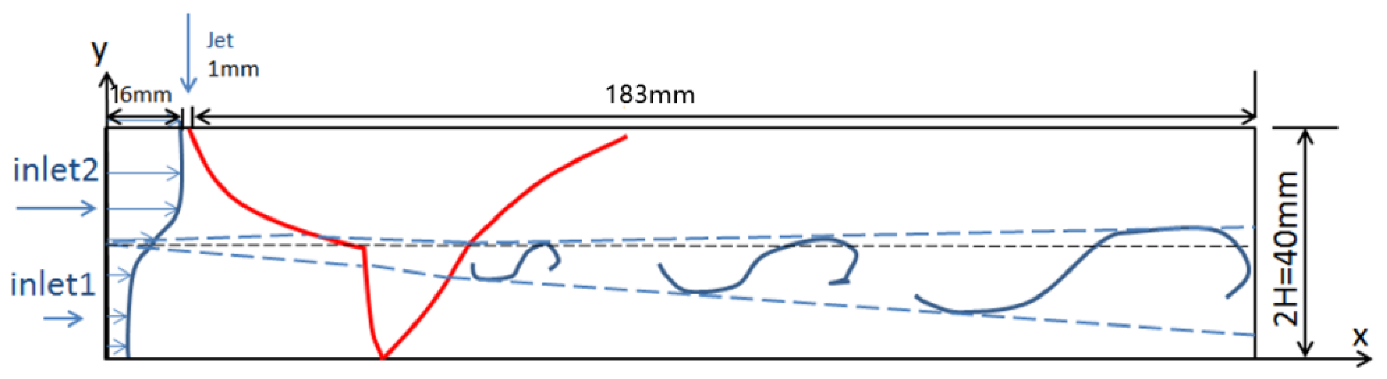
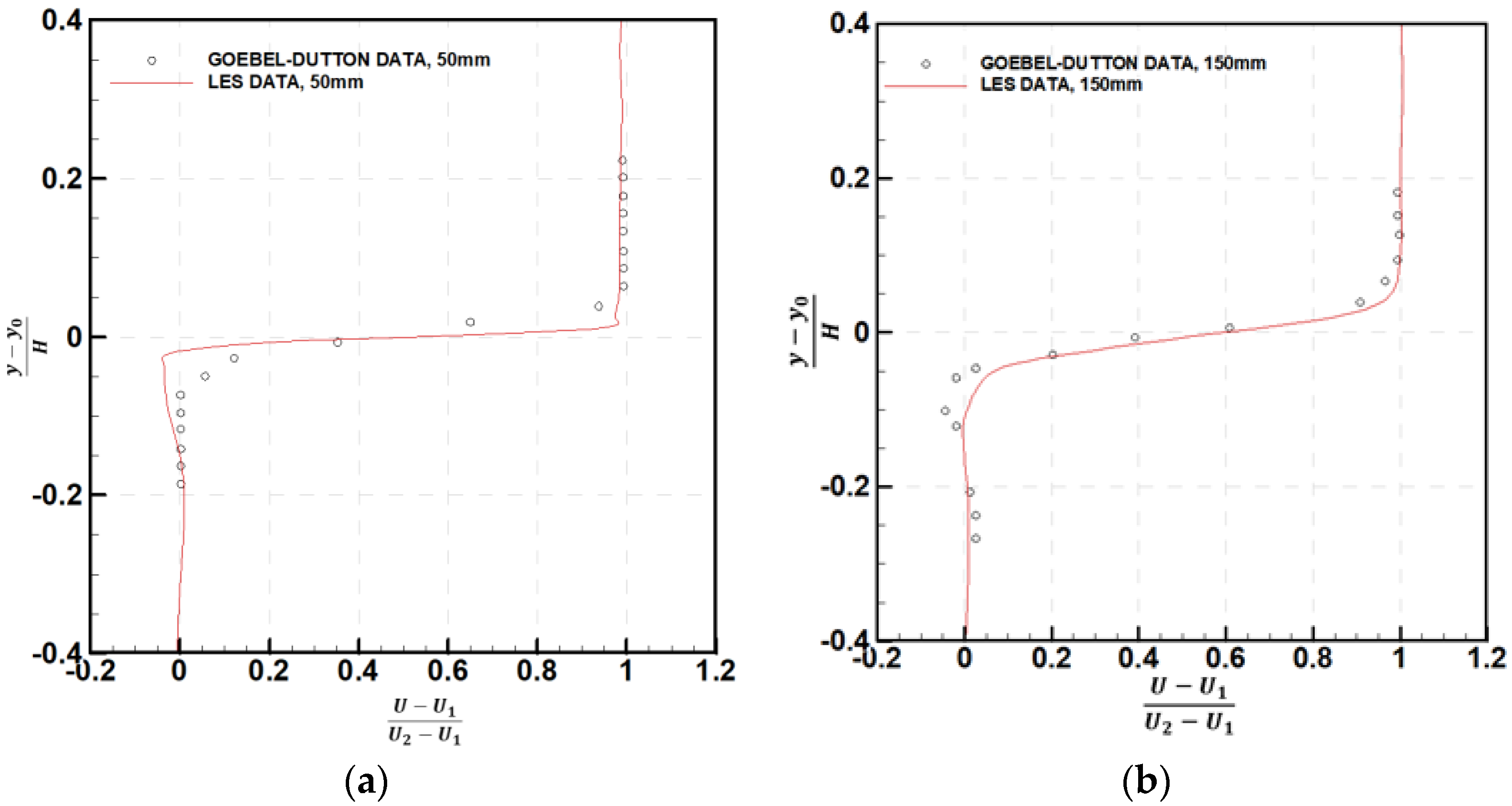
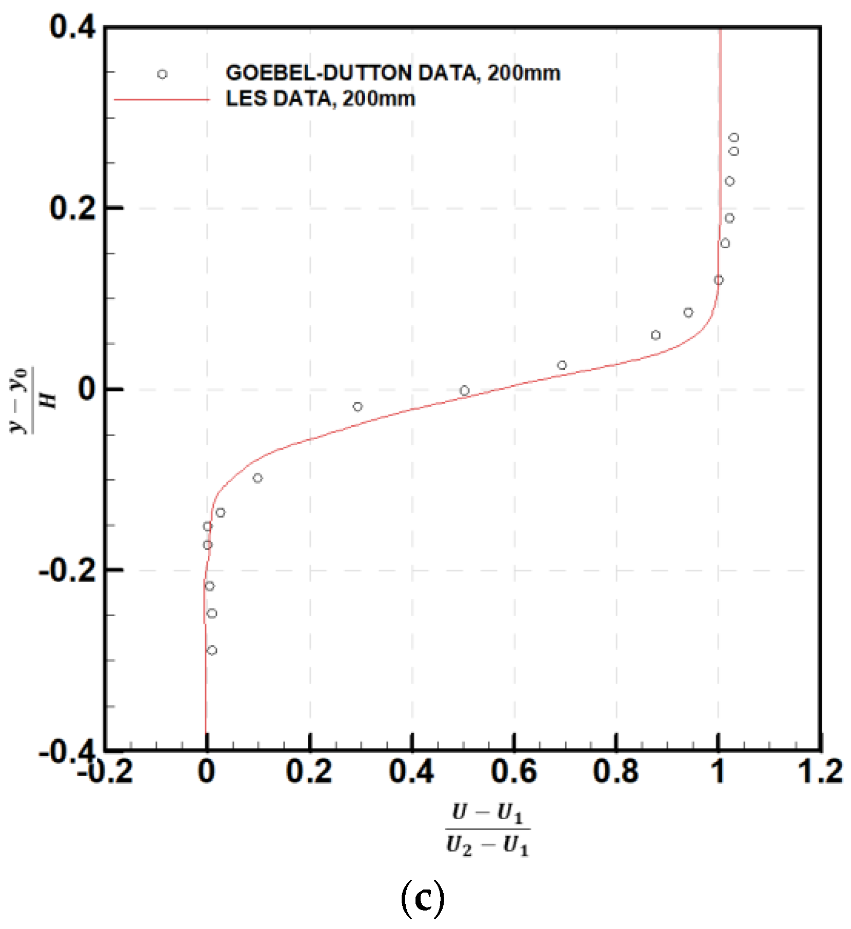
3.1. Flow Structure Visualization

The numerical schlieren technique proposed by Hadjadj [39] is employed here to obtain the instantaneous flow structures; it displays the flow field image based on density gradient. The strategy can be defined as
S x , y = β   e x p κ ρ ρ m a x
ρ = ( ρ x ) 2 + ( ρ y ) 2
Here, the parameter β determines the color corresponding to the zero gradient, the parameter κ governs the amplification degree of the small gradients, and the flow field is usually better displayed when the β and κ are taken as 0.8 and 15, respectively.
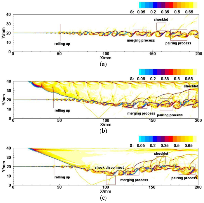
Figure 6 shows the numerical schlieren contour for present three cases. Due to the Kelvin–Helmholtz(K–H) instability generated by different upper- and lower-layer speeds, the typical coherent structure called K–H vortices in the mixing layer rolling up can be seen in all three cases. The K–H vortices gradually grow, and the phenomenon of pairing and merging between vortices appears. Browand [40] confirmed that the dynamic of pairing and merging between adjacent vortex structures is an important mechanism of free mixing layer growth. Apart from that, the shocklets in three cases are clearly visible. The shock waves generate by the local flow being impeded by the large-scale structure in the turbulent mixing layer when the local Mach number relative to the large-scale structure is greater than 1.0 [41]. Generally, shocklets appear in the high Mach number region of the flow field, corresponding to the upper flow area in our cases. It can be found that shocklets become more obvious due to the compression effect induced by jet shock in Case 2 and in Case 3.
In Case 1, the mixing layer develops around the central region of the flow field. However, in Case 2 and Case 3, due to the introduction of jet shock, the mixing layer is deflected downward after the incident shock, then deflected upward after the reflection shock. Meanwhile, the jet shock is first refracted through the mixing layer, then reflected upward on the lower wall, and then again refracted on the mixing layer. Refraction shock interacts with shocklets and finally becomes segmented state. Relative to Case 1, a new phenomenon of vortices rolling up closer to the inlet can be seen in Case 2 and Case 3, indicating that there are subsonic regions at the shock/mixing interaction area. This leads disturbance to transmit backward and can promote the vortices to roll up. Compared Case 2 with Case 3, it can be found that incident shock will be segmented in Case 2, while relatively straight in Case 3. Fast jet frequency in Case 2 makes the shock wave propagation speed lower than the jet disturbance speed, eventually it causes the ‘disconnection’ phenomenon. Overall, the vortex structures belonging to the interaction region possess characteristics of coexistence of both large- and small- scale vortices, and this dynamic is of great importance for promote mixing. Thus, detailed analysis concerning the structure behaviors is essential.
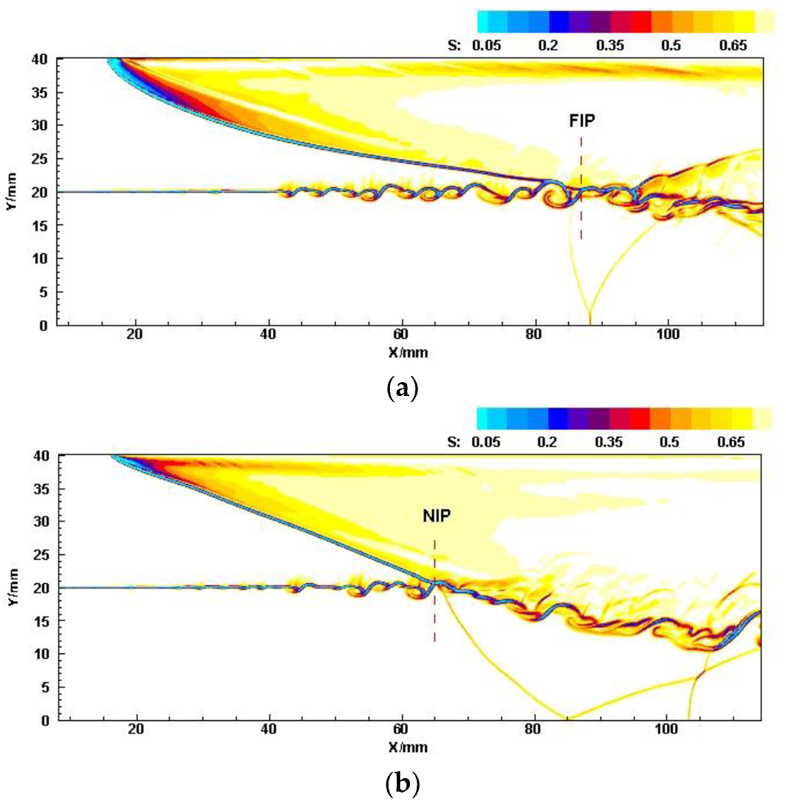
To better analyze the interaction process between jet shock and mixing layer in case 3, the detailed visualization around the interaction position is presented in Figure 7. One important phenomenon is that compared to the interaction process in case 2, in case 3 the interaction position is not fixed. In Figure 7a the interaction position located at x = 83 mm approximately, while in Figure 7b at about x = 62 mm. Indeed, by analyzing our calculated results it can be found that these two positions correspond to the farthest and nearest interaction locations in the flow field. Through reviewing previous literatures focusing on shock induced by wedge shock generator and its interaction process with mixing layer [23], it can be concluded that the interaction position was fixed and can be called the ‘point action mode’ (PAM). However, in present work new mode never reported before is found here and we defined it as ‘region action mode’ (RAM). This newly found mode plays important roles in the mixing enhancement process. Since as mentioned above, at different time the interaction point moves between the Farthest interaction point (FIP) and the nearest interaction point (NIP).
Numerous researches concerning mixing augmentation affected by wedge inducing oblique shock concluded that at the interaction point, the vortices distort and breakdown into small-scale structures [42]. This indicates that in present work, different interaction points induced by WJISW in a low frequency condition can result in the unique dynamical behaviors of vortex structures located between NIP and FIP. These dynamical behaviors including breakdown and deformation of vortex structure. The breakdown of vortex structure is related to the turbulent fluctuation of the flow field. Next, we clarify the relationship between the unique dynamic behavior of the vortex structure in RAM and the fluctuation characteristics of the flow field by quantitatively analyzing the distribution of the turbulent intensity of the flow field.

3.2. Turbulence Intensity Analysis

The turbulence intensity reflects the momentum exchange characteristics on both sides of the interface caused by the motion of fluid particle. Larger turbulence intensity means more significant three-dimensional characteristics of the flow, and large-scale structures are easily broken into small-scale structures [
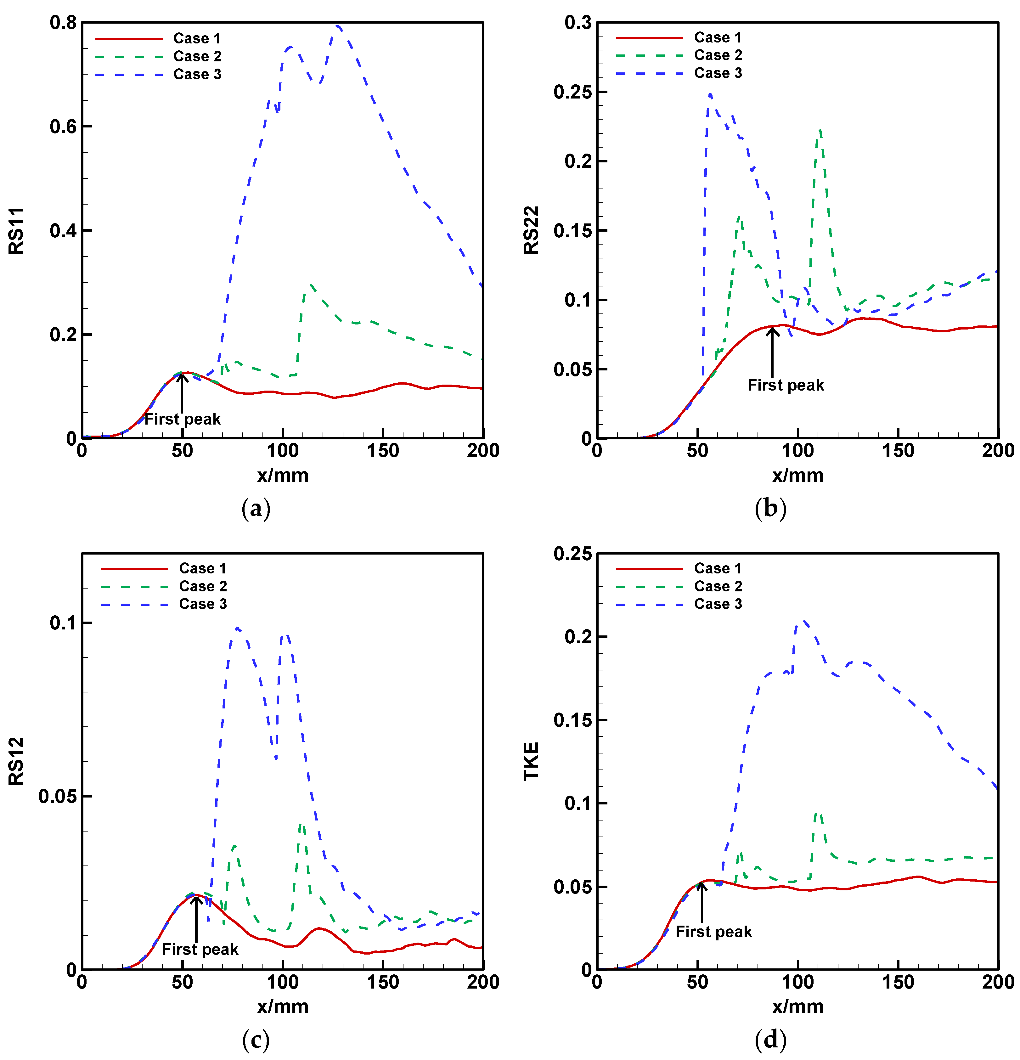
43]. In order to further explore the relationship between the unique dynamic behavior of the vortex and the turbulent fluctuation characteristics of the flow field under RAM, the distribution of maximum turbulence intensity at intersecting surface versus the streamwise x-direction and its integration over the entire streamwise x-direction are compared and analyzed for the three cases, as shown in Figure 8 and Figure 9, respectively.
The turbulence intensity characterized by four indexes, including the dimensionless streamwise Reynolds normal stress ( R S 11 ), transverse Reynolds normal stress ( R S 22 ), Reynolds shear stress ( R S 12 ), and turbulent kinetic energy ( T K E ) are calculated as follows,
R S 11 = ρ ¯ u u ˜ ρ 1 Δ u 2
R S 22 = ρ ¯ v v ˜ ρ 1 Δ u 2
R S 12 = ρ ¯ u v ˜ ρ 1 Δ u 2
T K E = 1 2 u u ˜ + v v ˜ Δ u 2
Here, ρ ¯ is the average density, ρ 1 is the density of lower flow, u is streamwise pulsation velocity, v is transverse the pulsation velocity and Δ u is the velocity difference between upper and lower flow. It can be seen that all the turbulence intensity characteristic values of the benchmark case have ‘one peak’. The reason of ‘one peak’ is the roll-up of vortices in the flow field, and the strong shearing effect leads to large pulsations in the mixing layer, resulting in a peak in the turbulence intensity term at this location. Whereas, in both Case 2 and Case 3 two higher peaks are detected along the streamwise x direction due to the effect of incident and reflected shock waves. Previous researches demonstrated that this phenomenon of ‘multiple peaks’ [44] can significantly promote the mixing process, so shock wave is beneficial to mixing augmentation. By comparing Case 2 and Case 3, it can be found that the growth rate of turbulence intensity is almost the same in both cases. However, under the influence of the RAM in case 3, the area where the shock wave impacts on the mixing layer is larger, which makes the turbulence intensity peak higher and the range of large values of turbulence intensity wider. This distribution property indicates that the RAM has a considerable effect on the large-scale enhancement of turbulence intensity in the mixing layer. Comparing the distribution of different turbulence intensity characteristics in the streamwise x-direction, it can be seen that the turbulence intensity of R S 22 reaches the peak earlier than that of R S 11 in Case 3, making the enhancement of the transverse Reynolds stress peak in this condition is not as significant as that of the streamwise Reynolds stress. This is because the shock oscillation is in streamwise direction in the RAM. Thus, the effect on the transverse Reynolds stress is not significant. The decline after R S 12 reaches its peak is gentler than that of R S 22 . This is because the shear Reynolds stress is a combined measure of turbulent pulsations in both the streamwise and transverse directions, and the superposition of the streamwise delayed peak and the transverse trough makes the tangential Reynolds stress decrease more slowly. The development of turbulent kinetic energy along the streamwise direction is similar to the streamwise Reynolds stress, because the turbulent kinetic energy is the superposition of the streamwise and transverse Reynolds stress. Furthermore, the shock wave oscillated in streamwise x-direction causes the streamwise Reynolds stress to dominate the flow fluctuation.
In summary, the turbulence intensity in the area of shock interaction is significantly increased under the RAM, and that in other regions of the flow field can also be effectively increased. Combined with the numerical schlieren observed in Figure 6, it can be seen that the vortex structure is more fragmented in the region of large values of turbulent intensity in the flow field, which proves that the large-scale growth of turbulent intensity in the flow field under the RAM is the principal reason for the fragmentation of vortex structure in Case 3.
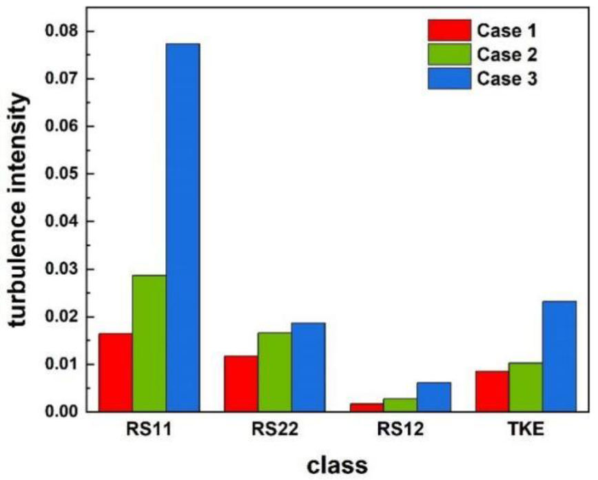
Integrating the turbulence intensity maximum values along the streamwise direction can reflect the turbulence characteristics of the whole flow field more clearly [44]. Figure 9 shows the comparison of the integrated values of R S 11 , R S 22 , R S 12 , and T K E along the streamwise x-direction for the three cases. It can be found that the value in Case 2 is slightly higher than that in Case 1, while the value in Case 3 is much higher than that in Case 2. In the comparison of the three cases in R S 22 , the difference between Case 3 and Case 2 is not much higher than the difference between Case 2 and Case 1. This is also consistent with the conclusion obtained from the above analysis of the distribution of the turbulence intensity maximum value along the streamwise x-direction. Therefore, considering the effect of enhancing the whole flow-field turbulence intensity, WJISW in a low frequency condition is much superior to WJISW in high frequency condition.

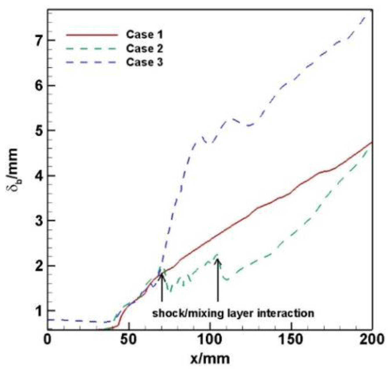
3.3. Mixing Layer Growth Process

To quantitatively evaluate the effect of WJISW on the mixing characteristics of the mixing layer, a velocity thickness index δ b is adopted, and it can be defined as the transverse distance between two positions with normalized mean velocity of 0.1 and 0.9,
δ b = y u ¯ = 0.9 y u ¯ = 0.1
where the normalized time-averaged velocity is defined as
u ¯ = U y U 1 U 2 U 1
The closer the normalized time-averaged velocity is to 1, the flow velocity is closer to the high-speed side and this position is more influenced by the high-speed side. The closer the normalized velocity is to 0, the closer the flow velocity is to the low-speed side, and this position is more influenced by the low-speed side. The distribution of velocity thickness versus streamwise x-direction for the three cases are depicted in Figure 10. The velocity thickness of the free mixing layer shows a linear growth characteristic, which is consistent with the results of previous work [42]. The velocity thickness in Case 2 decreases after two shock wave interaction points. Due to the compressibility of the shock wave, the shock wave causes a density increase, making the velocity thickness over a large area of the flow field in Case 2 smaller than that in Case 1. Nevertheless, the velocity thickness growth rate increases downstream of the shock interaction point, and it finally catches up with the velocity thickness of Case 1 at x = 200 mm. For Case 3, due to the unique advantage of the RAM, velocity thickness decreases after a long shock interaction zone. Particularly, velocity thickness increases steeply in the shock interaction zone owing to the dramatic increase in turbulence intensity at the shock interaction position, resulting in a sharp oscillation of the flow field. The increase in velocity thickness of the mixing layer in Case 2 at the shock interaction position is hardly noticed because the shock wave only acts on a single point in the mixing layer, which has little effect on the turbulence intensity of the flow field. Downstream of the shock interaction position, Case 3 has the same growth rate of velocity thickness as Case 2, and the final velocity thickness at x = 200 mm in Case 3 has increased by 62% compared to Case 1, which greatly improves the mixing level.
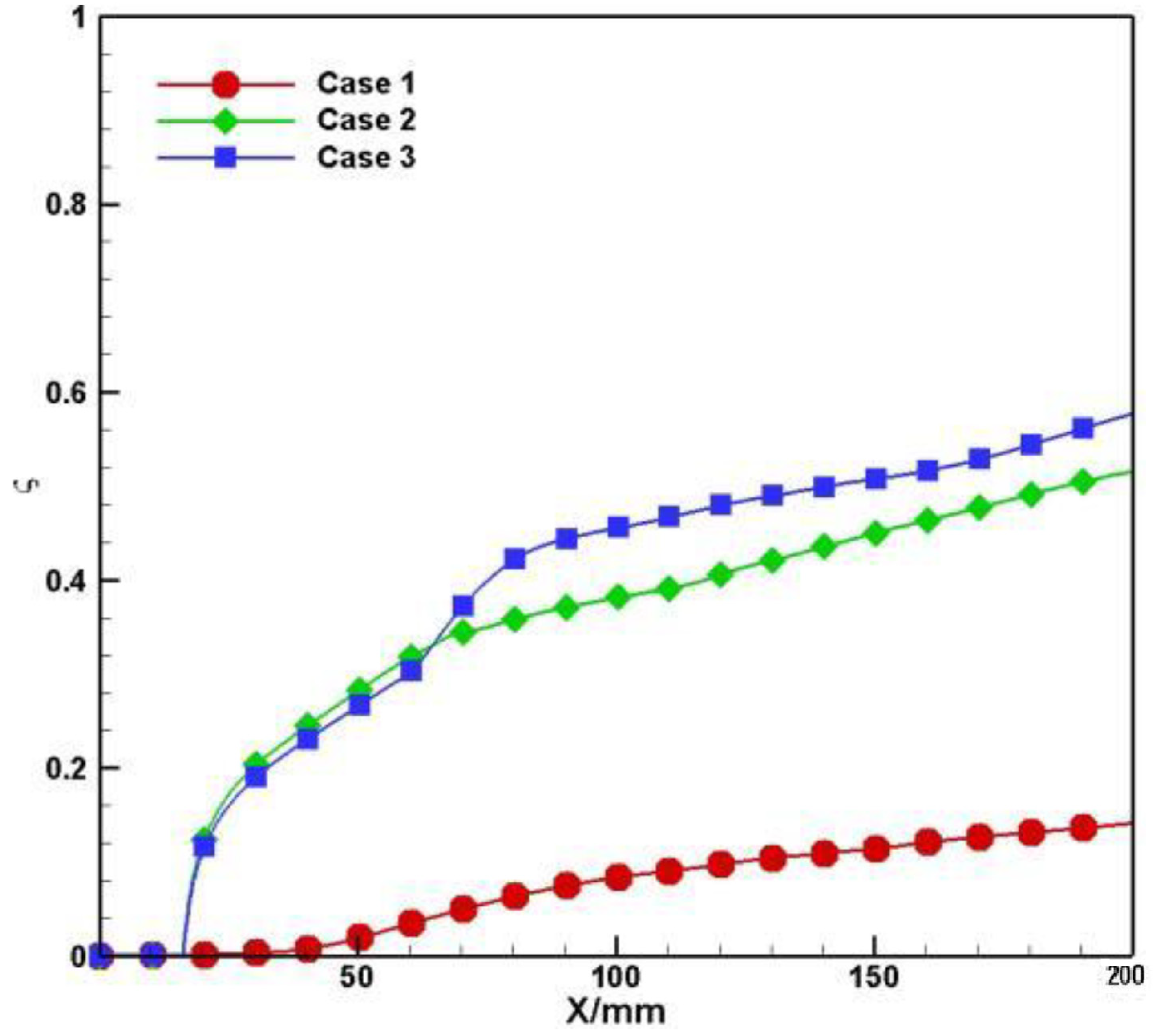
Because the interaction between shock wave and the mixing layer will cause the total pressure loss of the flow field, and the total pressure loss coefficient is an important index to evaluate the actual operation of the engine, we perform a detailed analysis of the total pressure loss coefficient, which is defined as,
ζ = 1 P x ρ udA P 0 ρ udA
where P x is the time-averaged total pressure of a certain streamwise position and P 0 is the time-averaged total pressure at the inlet position; ρ and u represent the time-averaged density and velocity, respectively. The total pressure loss distribution along the streamwise x direction for three cases is shown in Figure 11. It can be seen from the figure that when jet shock interacts with the mixing layer, although the total pressure loss coefficient increases to a large extent at the jet ejection position, the growth rate of the total pressure coefficient obviously slows down at x = 75 mm. Eventually, at x = 200 mm, the total pressure loss of Case 3 is larger than Case 2, and the total pressure loss of Case 2 is larger than Case 1. Notably, due to the introduction of shock waves, many techniques [45,46] for mixing enhancement cause a large loss in total pressure. In comparison, the flow loss of our scheme is acceptable. Besides, the total pressure loss of Case 3 is only slightly larger than that of Case 2, whereas Case 3 can achieve a higher mixing enhancement than Case 2. Therefore, in terms of comprehensive measurement of total pressure loss and mixing enhancement capacity, WJISW in a low frequency condition is a better choice.

3.4. DMD Analysis

As a newly proposed mixing technique, it can be found that the RAM generated by WJISW at a low frequency provides a significant degree of mixing enhancement, and the reveal of its mechanism contributes to the design optimization of the mixing augment device. In this paper, our cases are nonlinear dynamic systems, and the original flow field includes a large amount of information. Thus, it is not easy to grasp the focus of the data. It is worth noting that as an emerging reduced-order method applied in the flow field, DMD can realize the decomposition of the original data to obtain a specific flow field structure with a dominant frequency and growth rate [38]. This method can provide a convenient means for flow field dimensionality reduction and information acquisition, and it has achieved some application in the field of compressible flow [47,48,49,50], especially in revealing the typical structural characteristics of the flow [51]. In this paper, 1200 snapshots of the flow field with a time interval of 1.5μs are extracted from the transient flow field of three cases close to 8 circulation cycles for DMD analysis. The penalty terms Υ of the three cases in our paper are chosen as 1 × 10⁴, 1 × 10⁵, and 1 × 10⁴, respectively. After optimizing the amplitude of the modes by the DMD method, the number of non-zero modes of the three cases reduced from the original 1199 to 385, 423, and 401, respectively, which reflects the advantage of the DMD method in dimensionality reduction.
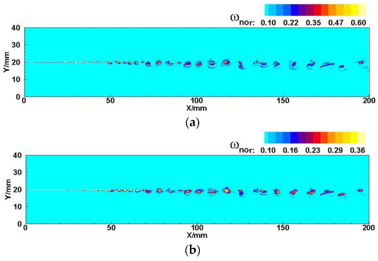
To confirm the reliability of the DMD method, the original flow field and the reconstructed flow field employing DMD method are compared and analyzed, as shown in Figure 12. The flow fields are characterized utilizing the dimensionless vorticity ω n o r and it can be defined as
ω n o r = ω z δ 0 u 2 u 1
ω z = u y v x
It can be seen that the DMD reconstructed flow field has basically restored the vortex behavior in the flow field, and the position and size also match with the original flow field. The roll-up, pairing, and merging of vortex structures can be clearly seen from the DMD reconstructed flow field, indicating that the vortex structure dynamics, which are important for the development of the mixing layer, can be captured by the DMD method.
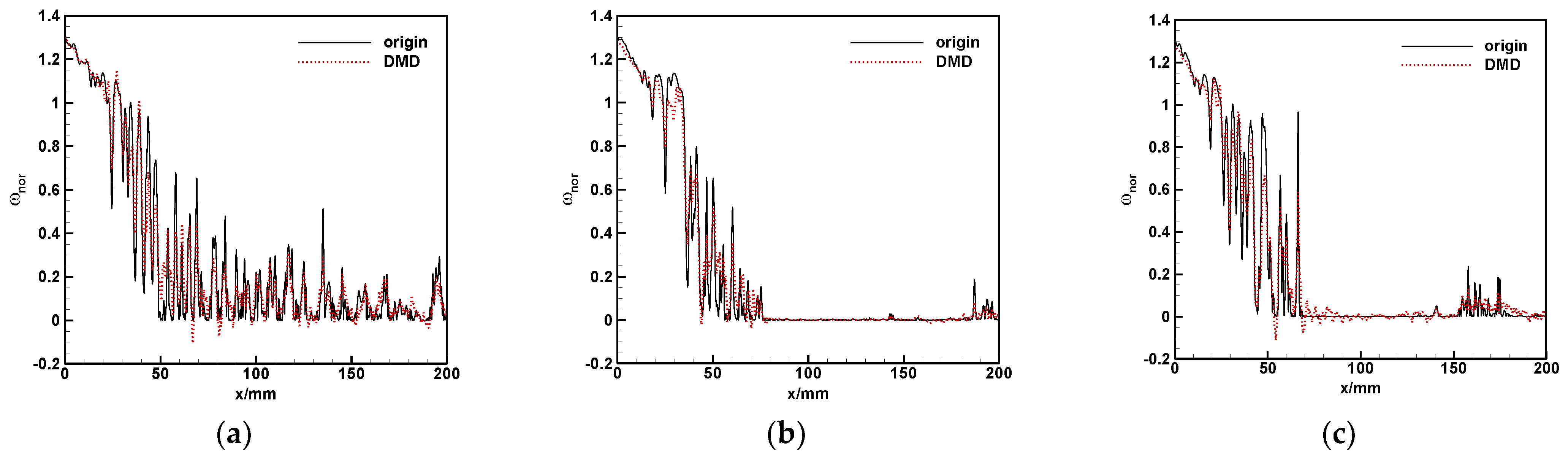
Furthermore, a quantitative comparison is performed by extracting the dimensionless vorticity on the centerline of the reconstructed flow field and the original flow field, as shown in Figure 13. From the figure, it can be more intuitively seen that the overall trend of the reconstructed values remains consistent with the original values, which also coincides with the results analyzed above. It can also be seen from the figure that the dimensionless vorticity on the centerline of the flow field of Case 1 fluctuates more, while Case 2 and Case 3 fluctuate less after x = 70 mm, which is due to the fact that the mixing layer impacted by WJISW will be deflected by the shock wave interaction, so the region of the most intense turbulent pulsation is not on the centerline of the flow field.
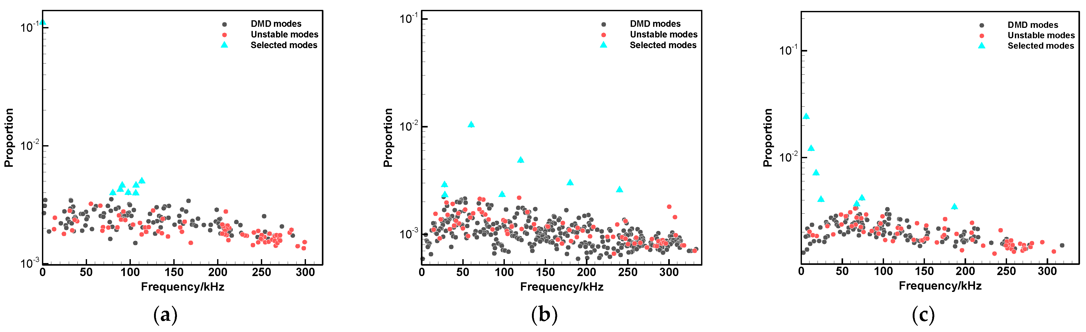
Figure 14 shows the frequencies and energy proportion distribution of DMD modes in three cases. Except for the first mode, all the modes are conjugate modes. The conjugate mode refers to modes with opposite frequencies, but with the same growth rate and modal energy proportion. Thus, here only frequencies greater than 0 are shown. The black points represent the values with eigenvalues less than or equal to 1 or a modal growth rate less than or equal to 0 (the two concepts can be found equivalent by simple logarithmic calculation), which correspond to stable or periodic modes, while the red points represent the values with eigenvalues greater than 1 or a modal growth rate greater than 0, which corresponds to unstable modes. Moreover, blue triangles correspond to the first eight modes with a higher energy proportion, which play dominant roles in the flow field and will be mainly analyzed below. It can be found that the frequency distribution of the first eight modes in Case 1 is concentrated around 100 kHz, while the frequency distribution of the first eight modes of Case 2 and Case 3 is more scattered, ranging from 50 kHz to 240 kHz and 6 kHz to 180 kHz, respectively. Meanwhile, it can also be seen that the frequencies of the first few modes in Case 3 are much smaller than those in Case 1 and Case 2.
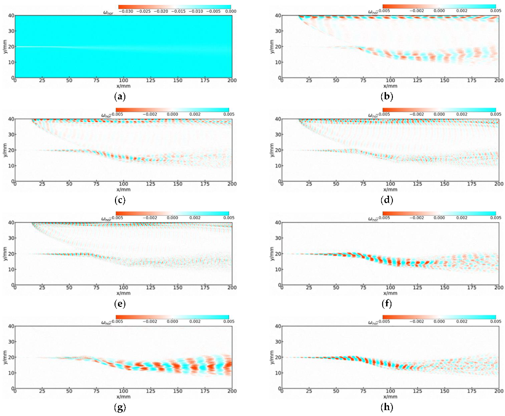
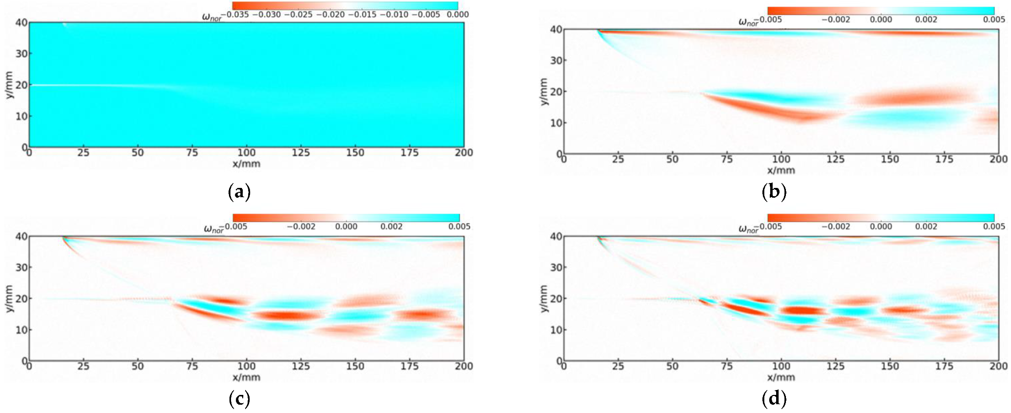
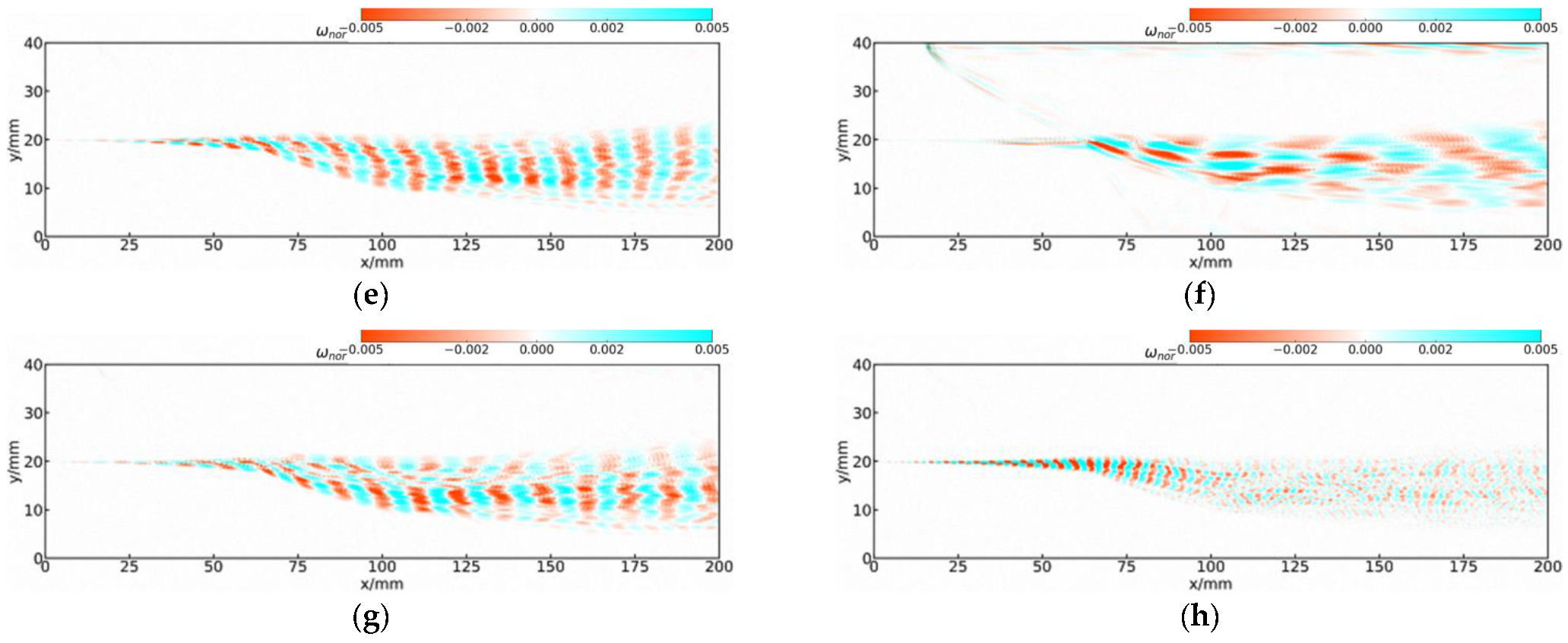
Figure 15, Figure 16 and Figure 17 show the first eight orders of spatial mode contours in three cases, respectively. The 1st modes show the time-averaged solution of dimensionless vorticity [52], while the rest of the modes reflect the oscillation characteristics generated by the flow field pulsation. The pulsation of the flow field in Case 1 mainly comes from the mixing of the fluid above and below the mixing layer, that is to say, the roll-up of K–H vortices. The upper and lower boundaries of the topology extracted from each mode can be regarded as the upper and lower boundaries of the mixing layer, and its width increases with the distance in streamwise x-direction, indicating that the thickness of the mixing layer grows in the streamwise x-direction. The analysis of the 2nd to 8th order modes shows that the topological structure, with alternating positive and negative values of dimensionless vorticity, appears only in the core region of the flow field. This structure can be considered as the spatial form of the wave, and the distance between the centers of positive and negative values can be regarded as half a wavelength [53]. The values in other regions of the flow field are zero, indicating that pulsations occur mainly in the mixing layer. Since the original flow field can be seen as a superposition of the DMD modes obtained from its decomposition, the vortices’ behavior can be seen in the superposition image. However, in the decomposed modes of different frequencies, only the wave structure can be seen in the flow field image. The above findings together converge to a conclusion that the vortex in the flow field is essentially a superposition of waves of different frequencies.
It can be seen from Figure 16 that the first few order modes in Case 2 cover a larger wavelength range than Case 1, and the 2nd, 3rd, 4th, and 5th order spatial modes of the flow field have significant shock effects, while the 6th, 7th, and 8th order spatial modes do not. This indicates that the 2nd, 3rd, 4th, and 5th order spatial modes of the flow field are shock-induced modes, and the energy of these modes accounts for a higher proportion of the total flow field energy compared to the later modes that are not shock-induced, i.e., K–H instability-induced modes. Therefore, the jet shock-induced modes play a dominant role in the flow field.
From Figure 17, we can see that the topology of the first few orders modes in Case 3 are very huge, especially the wavelength of the 2nd order mode has exceeded half of the flow field area. The 2nd, 3rd, 4th, and 6th order spatial modes can clearly see the effect of the shock wave, indicating that they are modes induced by jet shock wave, and the topological stratification can be seen more clearly than the other modes, induced only by K–H instability. Moreover, it can be clearly seen that the wavelengths of the modes induced by the shock are longer than those of the first two cases, but the wavelengths of these modes are varying in length. The modes with long wavelengths are favorable to induce large vortex structures, while the modes with short wavelengths are favorable to induce small vortex structures, resulting in the coexistence of large and small scales of vortex structures in the flow field. Entrainment and engulfment of large-scale structures allow surrounding fluids to enter the mixing region, and the nibbling effect of the small-scale structure facilitates the expansion of the surface area of scalar contact in the mixing layer. These dynamic behaviors accelerate the exchange of mass, momentum, and energy between the upper and lower layers of the flow [54], which is the reason why Case 3 has the best degree of mixing enhancement in the three cases. Comparing these three cases, Case 1 has a single vortex size, and Case 2 can induce different scales of vortex structures, but the largest vortex size is still small, and the large-scale entrainment effect is insufficient. Whereas, the interaction of large- and small-scale vortices in Case 3 leads to the fragmentation of the vortex structure in the flow field, which is consistent with the structure of the flow field in the numerical schlieren of Case 3.
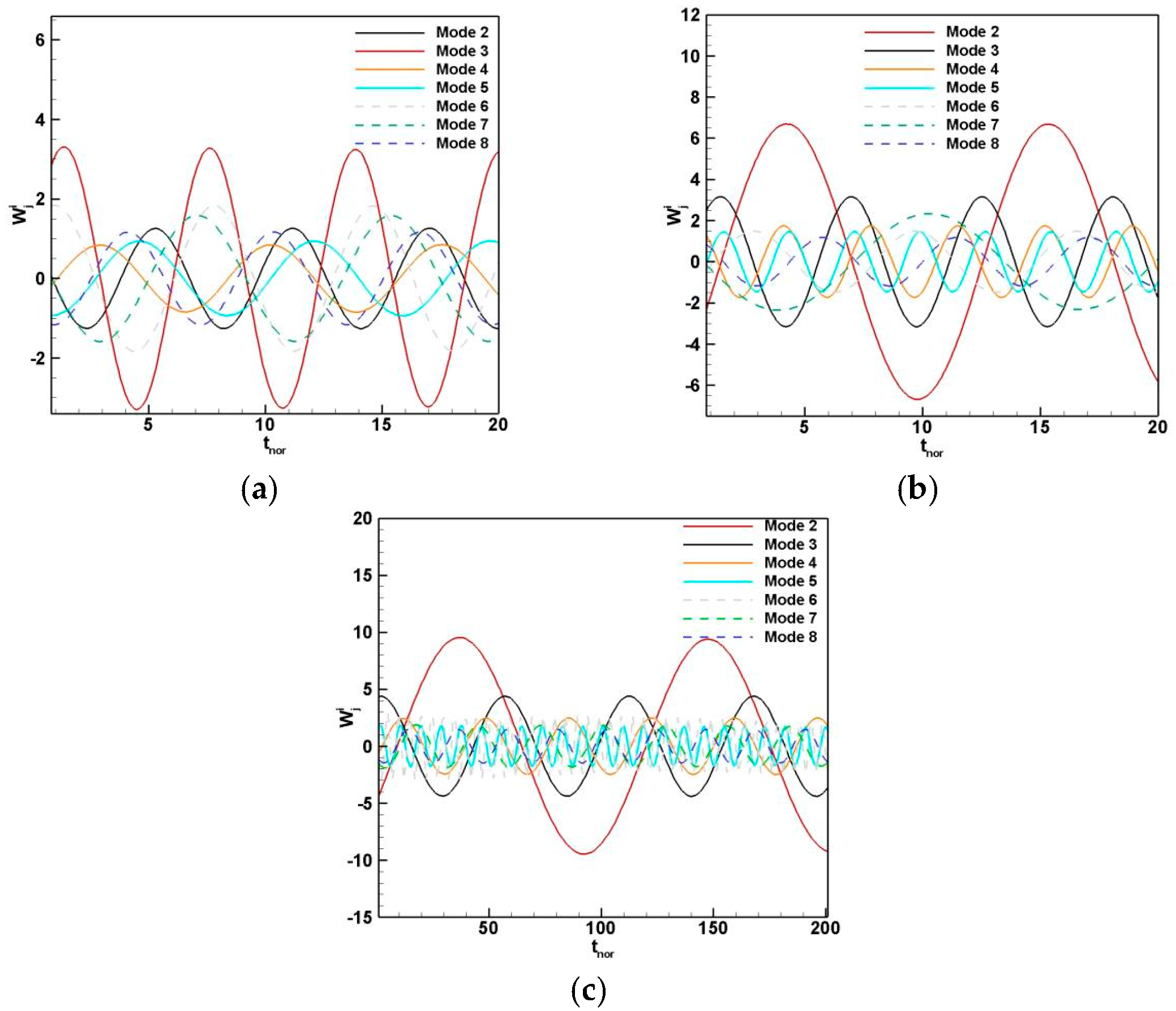
Figure 18 compares the evolution of the 2nd–8th order mode amplitudes with time in three cases. In the figure, the horizontal ordinate is the dimensionless time t n o r .
t n o r = t 0.0000015
From Figure 18a, it can be seen that there is not much difference between the modal amplitude and frequency of the first few order modes of Case 1 and the 2nd mode, which has a lower initial amplitude and is ranked ahead of the 3rd mode. This is because the DMD mode ranking criterion in this paper not only considers the initial amplitude, but also focuses on its evolution in the entire time history of available snapshots. The 3rd mode shows a weak decay characteristic with a negative growth rate, and the amplitude decreases slowly with time, while the 2nd mode is an unstable mode with a positive growth rate, and the amplitude increases gently with time. Therefore, the overall contribution of the 3rd mode to the flow field is greater than that of the 2nd mode, making the 2nd mode ranked before the 3rd mode, which also reflects the advantage of the modal ranking criterion in this paper. A large difference in the modal frequencies of the first few order modes of the flow field in Case 2 is presented in Figure 18b. Comparing with Figure 16, we can find that the mode with a small frequency corresponds to a long spatial mode wavelength and vice versa. The modes with the smallest frequencies and the longest spatial mode wavelengths are the 2nd mode and the 7th mode, respectively, and these structures are conducive to the induction of larger vortices in the flow field, which are found to be the modes induced by the jet shock and K–H instability, respectively, corresponding to Figure 16. However, the amplitude of the 2nd mode is more than twice that of the 7th mode, which also indicates that the modes induced by the jet shock are more dominant compared to those induced by K–H instability. It can be seen from Figure 18c that the frequencies of the first few order modes in the flow field in Case 3 are very different, corresponding to the larger wavelength range covered by the spatial modes in Figure 17. In addition, the 2nd mode amplitude is nearly twice as large as the remaining other modes, indicating that it accounts for a higher proportion of energy in the flow field.
The energy proportion, frequency, and growth rate of the first eight modes for three cases are analyzed to better research the vortex dynamics and mixing process. Table 6, Table 7 and Table 8 show the first eight orders of modal characteristics for the three cases, respectively. The frequencies of the first few modes of the flow field are high, except the 1st mode in Table 6. In addition, there is little difference in the 2nd- to 8th-order mode energy, suggesting that the energy in the flow field is dispersed, and no dominant modes control the development of the mixing layer.
From Table 7, we can see that the energy proportion of the first-order mode in Case 2 is 0.10638, which is lower than that in Case 1, which indicates that the perturbation energy proportion of Case 2 in the flow field is higher. Furthermore, the energy of the 2nd order and the 3rd order mode is much larger than the later modes, which indicates that these two modes of Case 2 are dominant in the flow field. Moreover, it can also be found that the energy of the 2nd, 3rd, 4th, and 5th order modes of the flow field are one, two, three, and four times of the wall jet frequency, respectively, which further confirms that the 2nd to 5th order modes are multiple frequency modes induced by the jet shock wave as mentioned above. It is noteworthy that the growth rate of the 2nd to 3rd order modes, which account for a relatively large amount of energy in the flow field, is negative and shows a weak decay, suggesting that the shock-induced modes will eventually decay completely if the flow field has a long streamwise length. In addition, although the 7th order mode is also induced by K–H instability, it has a smaller frequency and corresponds to a longer wavelength than the first few order modes in Case 1, perhaps due to the effect of the shock wave on the K–H instability of the flow field.
As can be seen from Table 8, the energy proportion of first-order mode in Case 3 is 0.05807, which is lower than that of both Case 1 and Case 2, indicating that the perturbations energy proportion of Case 3 in the flow field is higher. Similarly, the mode with multiple frequency of the jet ranks high in the energy proportion of each mode, which is the same as the conclusion reached in Case 2: the mode induced by the shock wave dominates the flow field. Moreover, the low frequency jet can excite high multiple frequency modes, suggesting that high frequency flow control can be achieved through low-frequency excitation. The decay rate of the 6th mode, which is a high-frequency mode with a mode frequency four times the excitation frequency, is found to be fast. As the decay rate of the higher multiple frequency mode is larger, the distance acting in the flow field is shorter, which provides a new idea to guide the design of the jet position. If the jet excitation is continuously introduced in front of the position where the higher multiple frequency mode decays more, the jet shock can interact on this position, which can make the low-frequency excitation mode and the high multiple frequency mode together dominate in the flow field, obviously enhancing the mixing degree.

4. Conclusions

In this paper, we research the mixing enhancement characteristics induced by the strategy of WJISW in a supersonic flow field through large eddy simulations. The instantaneous flow structures, turbulence pulsation characteristics, mixing layer growth process, and modal decomposition results are obtained and analyzed. In order to accentuate the mixing enhancement effect of this strategy, the free mixing layer under the same conditions is compared with it. The following conclusions can be drawn:
(1)
WJISW makes the mixing layer deflected. In particular, WJISW in a low frequency condition can result in the movement of the interaction position between NIP and FIP in the flow field. This new mode never reported before can be defined as ‘region action mode’ (RAM). In this mode, the vortex structures exhibit unique dynamic behavior, including breakdown and deformation. This is significantly different from the flow field of the mixing layer induced by a wedge shock generator;
(2)
The turbulence intensity of the mixing layer under WJISW appears multi-peak in the streamwise x-direction, which can significantly promote the mixing process. In addition, WJISW in a low frequency condition can make the turbulence intensity peaks higher in the streamwise x-direction and the range of large values wider, indicating that the ‘region action mode’ found in this paper has a considerable influence on the increase of turbulence intensity in the mixing layer, which significantly enhances the turbulent pulsation in the flow field;
(3)
The growth characteristics of the mixing layer under WJISW in a high frequency condition are similar to that of the mixing layer induced by wedge studied previously. The mixing layer thickness decreases after the shock interaction point, while the growth rate increases downstream, and eventually the mixing layer thickness will catch up with the free mixing layer. In contrast, under WJISW in a low frequency condition, the velocity thickness of the region where the shock wave acts with the mixing layer increases sharply, making the final velocity thickness increase by 62%, compared with the free mixing layer, and it greatly improves the mixing level;
(4)
The modal decomposition results show that the shock-induced modes dominate the flow field under WJISW. The coexistence of large- and small-scale structures in the mixing layer under WJISW in a low frequency condition is due to the dominance of the shock-induced modes. The entrainment and engulfment of large-scale structures promote surrounding fluids into the mixing region, and the nibbling effect of the small-scale structure facilitates the expansion of the surface area of scalar contact in the mixing layer, accelerating the exchange of mass, momentum, and energy between the upper and lower layers of the flow, both of which can effectively promote the mixing process;
(5)
The proposed strategy well shows the potential application in Scramjet and RBCC combustors for hypersonic propulsion systems. The newly observed ‘region interaction mode’ in the flow field influenced by wall-jet induced shock waves can obviously accelerate the mixing process. Future work concerning the optimization is essential to obtain a deeper understanding of the proposed strategy.

Author Contributions

Conceptualization, D.Z. and Y.W.; methodology, J.Z. and D.Y.; validation, J.Z. and Y.W.; writing—original draft preparation, J.Z.; writing—review and editing, D.Y., Y.W. and D.Z.; visualization, D.Y. and Y.W.; funding acquisition, D.Z. All authors have read and agreed to the published version of the manuscript.

Funding

This research was funded by the National Natural Science Foundation of China (Grant No. 12002372), Natural Science Foundation of Hunan Province (Grant No. 2021JJ40674), Excellent Postdoctoral Innovative Talents Project of Hunan Province (2021RC2067), and Scientific Research Project of NUDT (Grant No. ZK19-17).

Institutional Review Board Statement

Not applicable.

Informed Consent Statement

Not applicable.

Data Availability Statement

Not applicable.

Conflicts of Interest

The authors declare no conflict of interest.

References

  1. Lobo, J.U. Supersonic combustion in air-breathing propulsion systems for hypersonic flight. Annu. Rev. Fluid Mech. 2018, 50, 593–627. [Google Scholar]
  2. Bowersox, R.; Schetz, J.A. Compressible turbulence measurements in a high-speed high-Reynolds-number mixing layer. AIAA J. 1994, 32, 758–764. [Google Scholar] [CrossRef]
  3. Miller, M.F.; Bowman, C.T.; Mungal, M.G. An experimental investigation of the effects of compressibility on a turbulent reacting mixing layer. J. Fluid Mech. 2000, 356, 25–64. [Google Scholar] [CrossRef]
  4. Aupoix, B. Modelling of compressibility effects in mixing layers. J. Turbul. 2004, 5, 1–17. [Google Scholar] [CrossRef]
  5. Tan, J.; Zhang, D.; Lv, L. A review on enhanced mixing methods in supersonic mixing layer flows. Acta Astronaut. 2018, 152, 310–324. [Google Scholar] [CrossRef]
  6. Tillman, T.G.; Patrick, W.P.; Paterson, R.W. Enhanced mixing of supersonic jets. J. Propul. Power 1991, 7, 1006–1014. [Google Scholar] [CrossRef]
  7. Clayton, R.; Diego, R.; Capriotti, P.; Guy, R.W. Experimental supersonic combustion research at NASA langley. In Proceedings of the 20th AIAA Advanced Measurement and Ground Testing Technology Conference, Hampton, VA, USA, 15–18 June 1998. [Google Scholar]
  8. Burnes, R.; Parr, T.P.; Wilson, K.J.; Yu, K. Investigation of supersonic mixing control using cavities—Effect of fuel injection location. In Proceedings of the 36th AIAA/ASME/SAE/ASEE Joint Propulsion Conference and Exhibit, Las Vegas, NV, USA, 24–28 July 2000. [Google Scholar]
  9. Zang, A.; Tempel, T.; Yu, K.; Buckley, S. Experimental characterization of cavity-augmented supersonic mAnnual Review of Fluid Mechanicsixing. In Proceedings of the 43rd AIAA Aerospace Sciences Meeting and Exhibit, Reno, NV, USA, 10–13 January 2005. [Google Scholar]
  10. Choubey, G.; Pandey, K.M. Effect of parametric variation of strut layout and position on the performance of a typical two-strut based scramjet combustor. Int. J. Hydrog. Energy 2017, 42, 10485–10500. [Google Scholar] [CrossRef]
  11. Cao, D.; He, G.; Fei, Q.; Wei, X.; Lei, S.; Bing, L.; Huang, Z. LES study on flow features of the supersonic mixing layer affected by shock waves. Int. Commun. Heat Mass 2017, 85, 114–123. [Google Scholar] [CrossRef]
  12. Raman, G.; Rice, E.J. Supersonic jet mixing enhancement using impingement tones from obstacles of various geometries. AIAA J. 1995, 33, 454–462. [Google Scholar] [CrossRef]
  13. Gaitonde, D.V.; Samimy, M. Coherent structures in plasma-actuator controlled supersonic jets: Axisymmetric and mixed azimuthal modes. Phys. Fluids 2011, 23, 816–822. [Google Scholar] [CrossRef]
  14. Bidan, G.; Nikitopoulos, D.E. On steady and pulsed low-blowing-ratio transverse jets. J. Fluid Mech. 2013, 714, 393–433. [Google Scholar] [CrossRef]
  15. Strykowski, P.; Krothapalli, A.; Wishart, D. The enhancement of mixing in high-speed heated jets using a counterflowing nozzle. AIAA J. 1993, 31, 2033–2038. [Google Scholar] [CrossRef]
  16. Zhang, D.; Tan, J.; Liang, L.; Wang, Q. Visualization of flow structures and mixing characteristics induced by forced vibration in supersonic mixing layer. J. Vis. 2016, 19, 179–182. [Google Scholar] [CrossRef]
  17. Zhang, D.; Tan, J.; Liang, L. Investigation on flow and mixing characteristics of supersonic mixing layer induced by forced vibration of cantilever. Acta Astronaut. 2015, 117, 440–449. [Google Scholar] [CrossRef]
  18. Suzuki, H.; Kasagi, N.; Suzuki, Y. Active control of an axisymmetric jet with distributed electromagnetic flap actuators. Exp. Fluids 2004, 36, 498–509. [Google Scholar] [CrossRef]
  19. Marble, F.E. Progress toward shock enhancement of supersonic combustion processes. In Turbulent Reactive Flows; Springer: Berlin/Heidelberg, Germany, 1989. [Google Scholar]
  20. Menon, S. Shock-wave-induced mixing enhancement in scramjet combustors. In Proceedings of the 27th AIAA Aerospace Sciences Meeting, Reno, NV, USA, 9–12 January 1989. [Google Scholar]
  21. Lu, P.J.; Wu, K.C. On the shock enhancement of confined supersonic mixing flows. Phys. Fluids A Fluid Dyn. 1991, 3, 3046–3062. [Google Scholar] [CrossRef]
  22. Shau, Y.R.; Dolling, D.S.; Choi, K.Y. Organized structure in a compressible turbulent shear layer. AIAA J. 1993, 31, 1398–1405. [Google Scholar] [CrossRef]
  23. Génin, F.; Menon, S. Studies of shock/turbulent shear layer interaction using Large-Eddy Simulation. Phys. Fluids 2010, 39, 800–819. [Google Scholar] [CrossRef]
  24. Murugappan, S.; Gutmark, E.; Carter, C. Control of Penetration and Mixing of an Excited Supersonic Jet into a Supersonic Cross Stream (Postprint). Phys. Fluids 2005, 17, 1–13. [Google Scholar] [CrossRef] [Green Version]
  25. Techer, A.; Moule, Y.; Lehnasch, G.; Mura, A. Mixing of Fuel Jet in Supersonic Crossflow: Estimation of Subgrid-Scale Scalar Fluctuations. AIAA J. 2018, 56, 465–481. [Google Scholar] [CrossRef]
  26. Hafsteinsson, H.E.; Eriksson, L.E.; Andersson, N.; Cuppoletti, D.R.; Gutmark, E. Noise Control of Supersonic Jet with Steady and Flapping Fluidic Injection. AIAA J. 2015, 53, 1–22. [Google Scholar] [CrossRef]
  27. Gerdroodbary, M.B.; Takami, M.R.; Heidari, H.R.; Fallah, K.; Ganji, D.D. Comparison of the single/multi transverse jets under the influence of shock wave in supersonic crossflow. Acta Astronaut. 2016, 123, 283–291. [Google Scholar] [CrossRef]
  28. Ben-Yakar, A.; Mungal, M.G.; Hanson, R.K. Time evolution and mixing characteristics of hydrogen and ethylene transverse jets in supersonic crossflows. Phys. Fluids 2006, 18, 026101. [Google Scholar] [CrossRef] [Green Version]
  29. Semlitsch, B.; Cuppoletti, D.R.; Gutmark, E.J.; Mihăescu, M. Transforming the Shock Pattern of Supersonic Jets Using Fluidic Injection. AIAA J. 2019, 57, 1851–1861. [Google Scholar] [CrossRef] [Green Version]
  30. Germano, M. Turbulence—The filtering approach. J. Fluid Mech. 1992, 238, 325–336. [Google Scholar] [CrossRef]
  31. Ren, Z.; Wang, B.; Zheng, L. Numerical analysis on interactions of vortex, shock wave, and exothermal reaction in a supersonic planar shear layer laden with droplets. Phys. Fluids 2018, 30, 036101. [Google Scholar] [CrossRef]
  32. Li, H.; Tan, J. Cluster-based Markov model to understand the transition dynamics of a supersonic mixing layer. Phys. Fluids 2020, 32, 1–22. [Google Scholar]
  33. Yee, H.C.; Sandham, N.D.; Djomehri, M.J. Low-dissipative high-order shock-capturing methods using characteristic-based filters. J. Comput. Phys. 1999, 150, 199–238. [Google Scholar] [CrossRef] [Green Version]
  34. Kim, J.H.; Yoon, Y.; Jeung, I.S.; Huh, H.; Choi, J.Y. Numerical Study of Mixing Enhancement by Shock Waves in Model Scramjet Engine. AIAA J. 2003, 41, 1074–1080. [Google Scholar] [CrossRef]
  35. Goebel, S.G.; Dutton, J.C. Experimental study of compressible turbulent mixing layers. AIAA J. 1991, 29, 538–546. [Google Scholar] [CrossRef]
  36. Smirnov, N.N.; Betelin, V.B.; Nikitin, V.F.; Stamov, L.I.; Altoukhov, D.I. Accumulation of errors in numerical simulations of chemically reacting gas dynamics. Acta Astronaut. 2015, 117, 338–355. [Google Scholar] [CrossRef]
  37. Celik, I.B.; Ghia, U.; Roache, P.J.; Freitas, C.J.; Coleman, H.; Raad, P.E. Procedure for Estimation and Reporting of Uncertainty due to Discretization in CFD Applications. J. Fluids Eng. 2008, 130, 078001–078004. [Google Scholar]
  38. Rowley, C.W.; Mezić, I.; Bagheri, S.; Schlatter, P.; Henningson, D.S. Spectral analysis of nonlinear flows. J. Fluid Mech. 2009, 641, 115. [Google Scholar] [CrossRef] [Green Version]
  39. Hadjadj, A.; Kudryavtsev, A. Computation and visualization flow in high speed aerodynamics. J. Turbul. 2005, 6, 33–81. [Google Scholar] [CrossRef]
  40. Browand, F.K.; Latigo, B.O. Growth of the two-dimensional mixing layer from a turbulent and nonturbulent boundary layer. Phys. Fluids 1979, 22, 1011. [Google Scholar] [CrossRef]
  41. Zhao, Y.; Yi, S.; He, L.; Cheng, Z.; Tian, L. The experimental research of shocklet in supersonic turbulent mix layer. J. Natl. Univ. Def. Technol. 2006, 29, 12–15. [Google Scholar]
  42. Li, Z.; Jaberi, F. Numerical investigations of shock-turbulence interaction in a planar mixing layer. In Proceedings of the 48th AIAA Aerospace Sciences Meeting Including the New Horizons Forum and Aerospace Exposition, Orlando, FL, USA, 4–7 January 2010. [Google Scholar]
  43. Barre, S.; Bonnet, J.P. Detailed experimental study of a highly compressible supersonic turbulent plane mixing layer and comparison with most recent DNS results: Towards an accurate description of compressibility effects in supersonic free shear flows. Int. J. Heat Fluid Flow 2015, 51, 324–334. [Google Scholar] [CrossRef]
  44. Zhang, D.; Tan, J. Characteristics of enhanced mixing induced by plate jet actuation in supersonic flow. Phys. Fluids 2022, 34, 046112. [Google Scholar] [CrossRef]
  45. Vinogradov, V.; Shikhman, Y.; Albegov, R.; Vedeshkin, G. Experimental Research of Pre-Injected Methane Combustion in High-Speed Subsonic Airflow. In Proceedings of the AIAA International Space Planes & Hypersonic Systems & Technologies, Norfolk, VA, USA, 15–19 December 2003. [Google Scholar]
  46. Gerlinger, P.; Stoll, P.; Kindler, M.; Schneider, F.; Aigner, M. Numerical investigation of mixing and combustion enhancement in supersonic combustors by strut induced streamwise vorticity. Aerosp. Sci. Technol. 2008, 12, 159–168. [Google Scholar] [CrossRef] [Green Version]
  47. He, G.; Wang, J.; Pan, C. Initial growth of a disturbance in a boundary layer influenced by a circular cylinder wake. J. Fluid Mech. 2013, 718, 116–130. [Google Scholar] [CrossRef]
  48. Wan, Z.; Zhou, L.; Wang, B.; Sun, D. Dynamic mode decomposition of forced spatially developed transitional jets. Eur. J. Mech. B-Fluid 2015, 51, 16–26. [Google Scholar] [CrossRef]
  49. Ducoin, A.; Loiseau, J.C.; Robinet, J.C. Numerical investigation of the interaction between laminar to turbulent transition and the wake of an airfoil. Eur. J. Mech. B-Fluid 2016, 57, 231–248. [Google Scholar] [CrossRef] [Green Version]
  50. Scharnowski, S.; Kaehler, C.J.; Bolgar, I.; Statnikov, V.; Schroeder, W. Analysis of characteristic wake flow modes on a generic transonic backward-facing step configuration. Eur. J. Mech. B-Fluid 2016, 59, 124–134. [Google Scholar]
  51. Pirozzoli, S.; Bernardini, M.; Marié, S.; Grasso, F. Early evolution of the compressible mixing layer issued from two turbulent streams. J. Fluid Mech. 2015, 777, 196–218. [Google Scholar] [CrossRef] [Green Version]
  52. Gao, C.; Zhang, W.; Ye, Z. Numerical study on closed-loop control of transonic buffet suppression by trailing edge flap. Comput. Fluids 2016, 132, 32–45. [Google Scholar] [CrossRef]
  53. Murray, N.; Sällström, E.; Ukeiley, L. Properties of subsonic open cavity flow fields. Phys. Fluids 2009, 21, 095103. [Google Scholar] [CrossRef]
  54. Jahanbakhshi, R.; Vaghefi, N.S.; Madnia, C.K. Baroclinic vorticity generation near the turbulent/ non-turbulent interface in a compressible shear layer. Phys. Fluids 2015, 27, 105105. [Google Scholar] [CrossRef]
Figure 1. Schematic of calculation model and flow field structure. (The red solid line represents the position of the jet shock wave in the flow field, the area between the blue dotted lines is the mixing layer, and the blue arrow represents the incoming flow and the wall jet respectively).
Applsci 12 08384 g001
Figure 2. Computational mesh distribution.
Applsci 12 08384 g002
Figure 3. Distribution of Mach number along the streamwise direction of the centerline of the flow field in different grid condition.
Applsci 12 08384 g003
Figure 4. Experimental schematic diagram of Goebel and Dutton.
Applsci 12 08384 g004
Figure 5. Comparison of time-averaged velocity profiles of mixing layers: (a) x = 50 mm; (b) x = 150 mm; (c) x = 200 mm.
Applsci 12 08384 g005aApplsci 12 08384 g005b
Figure 6. Instantaneous flow structures of present three cases: (a) Case 1; (b) Case 2; (c) Case 3.
Applsci 12 08384 g006
Figure 7. Evolution dynamics of local flow field: (a) t = t0; (b) t = t0 + 90 μs.
Applsci 12 08384 g007
Figure 8. Peak value of turbulence intensity along streamwise direction for three cases: (a) R S 11 ; (b) R S 22 ; (c) R S 12 ; (d) T K E .
Applsci 12 08384 g008
Figure 9. Integration of turbulence intensity along the streamwise direction for three cases.
Applsci 12 08384 g009
Figure 10. Comparison of velocity thickness of three cases.
Applsci 12 08384 g010
Figure 11. Pressure loss coefficient along streamwise direction for three cases.
Applsci 12 08384 g011
Figure 12. Comparison of original flow field and DMD reconstructed flow field: (a) original flow field of case 1; (b) constructed flow field of case 1.
Applsci 12 08384 g012
Figure 13. Comparison of original value and DMD reconstruction value of flow field center line: (a) case 1; (b) case 2; (c) case 3.
Applsci 12 08384 g013
Figure 14. Distribution of mode frequency and energy: (a) Case 1; (b) Case 2; (c) Case 3.
Applsci 12 08384 g014
Figure 15. Dimensionless vorticity contour of the first eight modes in Case 1: (a) the 1th mode; (b) the 2nd mode; (c) the 3rd mode; (d) the 4th mode; (e) the 5th mode; (f) the 6th mode; (g) the 7th mode; (h) the 8th mode.
Applsci 12 08384 g015
Figure 16. Dimensionless vorticity contour of the first eight modes in Case 2: (a) the 1st mode; (b) the 2nd mode; (c) the 3rd mode; (d) the 4th mode; (e) the 5th mode; (f) the 6th mode; (g) the 7th mode; (h) the 8th mode.
Applsci 12 08384 g016
Figure 17. Dimensionless vorticity contour of the first eight modes in Case 3: (a) the 1st mode; (b) the 2nd mode; (c) the 3rd mode; (d) the 4th mode; (e) the 5th mode; (f) the 6th mode; (g) the 7th mode; (h) the 8th mode.
Applsci 12 08384 g017aApplsci 12 08384 g017b
Figure 18. Evolution of time coefficients among seven dominant DMD modes: (a) Case 1; (b) Case 2; (c) Case 3.
Applsci 12 08384 g018
Table 1. Inflow parameters.
MaV/(m·s−1)P/kPaT/KMc
inlet11.7658.4101346.60.6
inlet25.6986.310176.7
Table 2. Simulation conditions for three cases.
Frequency of JetState of Jet Shock
Case 1Noneshock free
Case 22f0high-frequency shock
Case 30.2f0low-frequency shock
Table 3. Incoming condition of Geobel–Dutton experiment.
StreamMaV/(m·s−1)T/KP/kPaMc
11.9700334490.45
21.340021549
Table 4. Error estimates.
Allowable Error (%)Grid ResolutionNumber of Time StepsAccumulated ErrorAllowable Number of Time StepsReliability
53000 × 20072,0009.97 × 10−61.81 × 10122.51 × 107
Table 5. Sample calculation of discretization error.
N1, N2, N3 r 21 r 32 ϕ 1 ϕ 2 ϕ 3 p e a 32 G C I f i n e 32
750,000, 600,000, 300,0001.1181.414984.422984.3101983.86131.090.046%0.12%
Table 6. Modes’ characters of the first eight modes in Case 1.
OrderProportionFrequency/HzGrowth Rate
10.1109515 × 10−126
20.005012113,335255
30.004626106,678−1074
40.00462190,923575
50.00426188,690393
60.00400497,742−428
70.00398380,179−265
80.003970106,43089
Table 7. Modes’ characters of the first eight modes in Case 2.
OrderProportionFrequency/HzGrowth RateFrequency/fj
10.10638−8 × 10−112.650
20.0171660,000−401
30.00802119,998−502
40.00495179,999793
50.00421239,974924
60.0038597,445−251.62
70.0037552,148−6310.87
80.00359118,0781491.96
Table 8. Modes’ characters of the first eight modes in Case 3.
OrderProportionFrequency/HzGrowth RateFrequency/fj
10.05807−2 × 10⁻¹⁰−7.690
20.014026018−941
30.0070312,028102
40.0041318,055673
50.0024373,954−23912.32
60.0023924,025−3004
70.0023467,617−51111.26
80.00229186,742−22532.12
Publisher’s Note: MDPI stays neutral with regard to jurisdictional claims in published maps and institutional affiliations.

