Article

CPAP Adherence Assessment via Gaussian Mixture Modeling of Telemonitored Apnea Therapy

by
Jose F. Rodrigues, Jr.
1,*,
Sebastien Bailly
2,
Jean-Louis Pepin
2,
Lorraine Goeuriot
3,
Gabriel Spadon
4 and
Sihem Amer-Yahia
3
1
Institute of Mathematics and Computer Science, University of Sao Paulo, Sao Carlos 13566-590, SP, Brazil
2
Centre Hospitalier Universitaire, 38700 Grenoble, France
3
CNRS, University Grenoble Alpes, 38400 Saint-Martin d’Heres, France
4
Institute for Big Data Analytics, Dalhousie University, Halifax, NS B3H 4R2, Canada
*
Author to whom correspondence should be addressed.
Appl. Sci. 2022, 12(15), 7618; https://doi.org/10.3390/app12157618
Submission received: 22 April 2022 / Revised: 21 July 2022 / Accepted: 25 July 2022 / Published: 28 July 2022

Abstract

:
Sleep disorders pose serious cardiovascular threats if not treated effectively. However, adherence to Continuous Positive Airway Pressure (CPAP), the most recommended therapy, is known to be challenging to monitor. Telemonitored CPAP equipment has improved the follow-up of CPAP adherence (hours of use per night) by producing far larger amounts of data collected daily. The analysis of such data have relied on averaging the entire therapeutic history and interpreting it without a proper reference concerning the level of adherence. By contrast, we contribute with an unsupervised machine-learning methodology that (i) translates the adherence data to a scale of discrete numbers that hold correspondence to the most usual 30-day-long patterns as observed in a real-word database; (ii) avoids the loss of information aggregation problem by creating summaries of the time series that capture the dynamic nature of the everyday-use CPAP. Our experiments have detected eight particular adherence behaviors validated with information-oriented statistical criteria; we successfully applied them to the time series of a French hospital to produce summaries that reflect the adherence of any 30 days of interest. Our method can aid physicians in more precisely evaluating the therapy adherence, as well as fostering systems to alert of problems in the treatment automatically.

1. Introduction

Obstructive Sleep Apnea (OSA) is a disorder that appears due to obstructions of the upper airway while the patient is sleeping; the obstruction occurs as the dilator muscles and soft tissues of the pharyngeal wall collapse. OSA is characterized by at least five of these obstructive events per hour, followed by consequential symptoms, including daytime sleepiness, snoring, and choking arousals [1]. In the US alone, it is estimated that OSA afflicts nearly 30 million adults with a cost of diagnosing and treating of approximately US$12.4 billion in 2015 [2,3]. This condition can potentially reduce the quality of life and increase the risks of cardiovascular comorbidities [4]. Hence, it must be addressed by an effective treatment—Continuous Positive Airway Pressure (CPAP) therapy is the recommended course of action. However, adherence to CPAP is a medical concern; in a large study, ref. [5] investigated the adherence to treatment over 50 years considering 569 studies; the author found that sleep disorder therapies have the poorest adherence rate of nearly 65.5%. In this sense, Ref. [6] argued that the lack of adherence to CPAP might be justified by the development of alternative treatments, including surgery of the palate, which allows selected subjects to obtain excellent results even at the expense of initial suture extrusion. By contrast, the effect of non-benzodiazepine sedative hypnotics on CPAP adherence in patients with OSA has been evaluated in a systematic review and meta-analysis [7]. In another work, Ref. [8] mention that the acceptance of the CPAP therapy might be as low as 50%, with up to 25% of the patients giving up the treatment by the third year; these facts are signs of the importance of constantly monitoring how the patients adhere to the therapy.
Assessing adherence to CPAP is itself a challenge. The latest approach for evaluating CPAP use adherence comes from monitoring technologies wirelessly connected or telemonitoring. The potential for remote telemonitoring to restructure current care management paradigms is immense; it can be used to provide sleep-specialist care to patients in underserved areas, delivering more efficient, cost-effective, and accessible health care services beyond traditional office settings [9]. In the case of CPAP use, there is potential for reducing the number of clinic visits, improving home care, and early detection of problems [10]. Furthermore, such devices generate data to support the integrated care of comorbidities and self-management of sleep apnea [11].
The evaluation of CPAP adherence has been based on the average number of hours or minutes of use [12,13,14], which yields a rate of hours per night and a standard deviation. Such analysis considers entire periods of use, which are aggregated to one single value. However, CPAP use time series might carry much more information than a single value can express; as depicted in Figure 1, the patient behavior is complex. CPAP use time series present a high frequency of oscillations in the number of hours, and they are prone to events dictated by external facts that influence the sleep quality, leading the series to different tendencies along time. These facts make the use of simple aggregations ineffective and potentially misleading as they do not capture the dynamic natures of such data. Ref. [15] discuss the loss of information due to aggregation operations in series data, which they argue to be more critical in long-term series. In another work, Ref. [16] discusses the implications of the loss of effective estimation and testing power due to the discarded information after aggregation. For example, for Figure 1, the mean is 7.1 h +/−1.6, which is not able to express the struggling period of adaptation at the beginning, some ups and downs along with the series, and the latest crisis at the end of the series.
In this work, we propose an analytical process to characterize periods of CPAP use tackling two problems simultaneously: (i) we reduce the complexity of the time series by translating the adherence behavior to a scale of discrete numbers that hold correspondence to the most usual behaviors as observed in a real-word database; (ii) we avoid the loss of information aggregation problem by creating summaries of the time series that capture the dynamic nature of the everyday-use CPAP therapy. We focused only on CPAP adherence values (hours of use), independently of other attributes that can be collected by daily telemonitoring, such as leak, residual Apnea–Hypopnea Index (AHI), and/or baseline clinical markers. The methodology, nevertheless, applies directly to other attributes and should be the topic of future research.

2. Related Work

According to the work of [9], sleep medicine will look forward to big data as a means to massive health management, increased automated care delivery, patient self-care capabilities, predictive analytics for providing clinical decision support, peer-to-peer support opportunities, and effective real-time patient monitoring. Accordingly, remote monitoring of CPAP allows one to follow the progress of apnea and detect acute events, providing confidence to the patient and reducing the number of follow-up visits. Fulfilling these expectations requires efficient analytical methods; in the case of apnea monitoring, the challenge is to digest long series of telemonitoring signals. For this reason, it is arguable that physicians must consult patient data daily and react to alarms. However, according to [9] this is infeasible in countries such as the USA due to the busy work schedule of physicians.
In the context of assessing CPAP-based therapies, ref. [17] affirms the existence of heterogeneity between patients with OSA concerning comorbidities and symptoms. Following this hypothesis, ref. [18] used clustering techniques to detect OSA phenotypes (classes of patients) considering 13 clinical variables; next, they compared the five classes they found to clusters obtained with CPAP-treatment outcomes observed during 6 months of therapy. Their results indicated a strong agreement between the two sets of clusters, suggesting that cluster analysis is an opportunity for the clinical characterization of patients with OSA. We pursue this diagnosis approach by introducing a characterization of patients considering the time of CPAP use, a metric that points out how well the adherence to the therapy has been, and that we translate into a scale of discrete numbers. The work of [18] provides interesting insights regarding the relationship of CPAP use and clinical indicators; similarly to them, we use clustering techniques to find meaningful characterizations of apnea patients but, differently, we do not aggregate the CPAP outcome into one single value, neither we analyze the whole time series of CPAP therapy at once.
In the work of [19], the authors considered a cohort containing only patients with moderate to severe OSA, as indicated by the metric Apnea–Hypopnea Index (AHI) measured by polysomnography breathing monitoring, the gold standard for OSA diagnosis. Their goal was to detect the phenotypes in a universe of well-characterized OSA patients. Using hierarchical clustering methods over variables related to age, sex, symptoms, obesity, comorbidities, and environmental risk factors, they found six clusters, each with a statistically distinct profile. In common with our work, ref. [19] use unsupervised machine learning to characterize patients (phenotypes); differently, while they consider a snapshot of the patients’ clinical symptoms, we use the constant flow of telemonitoring data to characterize the course of periods of the CPAP therapy. The innovation of our approach comes from the dynamic nature of our method, which can capture the constant-changing circumstances of the therapy.
Reference [20] point out that, although AHI is the most used metric for OSA severity, it does not correlate well in all the clinical scenarios. Other signals might be useful for detecting endotypes, so to target treatments more precisely to specific patient traits. In a similar line of thought, we advocate that understanding other factors beyond AHI has the potential to assist the physician in determining the necessary therapy intervention [21]. Accordingly, we proceed by inspecting the CPAP use telemonitoring signal (hours of use), focusing on the characterization of the ups and downs, regularities, and irregularities during the patient’s adaptation to the therapy, allowing the physician to detect problems that require intervention.
Similar to our work, ref. [22] exploits the number of hours of CPAP use to characterize patients with respect to therapy adherence. In their methodology, they analyzed the series of 161 patients, each with nearly 180 nights of data; from each series, they extracted the average number of hours, level, slope, variance, and autocorrelation of the series. These features are then fed into a clustering process based on dynamic analysis [23]. As a result, they identified four clusters, which they named Great Users, Good Users, Low Users, and Slow Decliners. An immediate limitation of this work, and of the work of [24] (who identified seven clusters over only 71 patients), is the need to analyze time series of similar sizes. Since patients usually have different trajectories, just a few will satisfy similar temporal constraints, severely reducing the cohort cardinality. By contrast, we identify recurrent 30-day patterns observed in the realm of a much larger cohort with over 2000 patients; this approach allowed us to work with over 20,000 pattern instances, robust support for our analysis. Another problem is that the methods of [22,24] disregard the dynamic aspect of the patients when exposed to the CPAP therapy. By contrast, we assume that the efficacy of the therapy is subject to variations over time: at the beginning of the therapy, after years of use, during a period of stress, possibly accompanied by insomnia [25]; while treating another infirmity; and so on. Accordingly, our method is designed to characterize shorter periods of 30 days or any other size as the analyst desires. Lastly, using a sliding-window method, we summarize a given patient’s time series to simplify the process of inspecting the entire period of therapy.
In the state of the art, we found that many works have sought to characterize OSA patients into groups, or clusters, of individuals with similar clinical signals or therapy outcomes. Since this is an unsupervised task, the various works provide sets of groups with different cardinalities and characterizations. This variability is explained by factors such as cohort peculiarities, methodology specificities, and result interpretation. Although the discrepancy is not desirable, these many works still point to an intersection of relevant aspects: (i) the patients indeed behave in a stratified manner, (ii) the characterized behaviors are interpretable from heterogeneous perspectives, and (iii) there is a meaningful aspect in characterizing patients, which has motivated the very investigation of the topic. In this work, we touch upon the same investigative line, but from the prospect of the time of CPAP use, a straight indicator of treatment adherence. We innovate by assuming that the different periods of CPAP therapy deserve, each one, a distinguished analysis; in contrast to former works that aggregate the whole therapeutic history of a given patient into a single average. With this course of action, we introduce a method able to summarize long-term CPAP use series without resorting to aggregation methods but, instead, introducing a scale of discrete numbers that hold, as referential, the most usual 30-day-long periods observed in a real-world database.

3. The CPAP Use Dataset

Dataset CPAP use comes from a home care provider located in the city of Grenoble, France. It is concerned with the treatment of sleep apnea, including the equipment (CPAP brand and model), the telemonitoring data produced by the equipment, follow-up appointments, and corresponding readings—the CPAP use dataset is populated daily. For the rest of this work, we analyze the daily number of hours of CPAP use automatically reported by each piece of equipment via telemonitoring and stored at dataset CPAP use. Our instance of the dataset comprises 3209 patients, of which we discarded those with less than 180 days of monitoring (similar to [22]), resulting in a dataset with 2381 patients. Figure 2a presents the dataset’s distribution concerning the number of days of monitoring. We also discarded patients whose average number of hours is less than 2.5 h or higher than 10.0 h; that is, the tails of the normal distribution presented in Figure 2b.

4. Methodology

Our goal is a method able to translate 30 days of CPAP use into one single number that summarizes the patient adherence within a referential scale. This method can be used over the whole time series of a given patient as a sliding window that simplifies the interpretation of the usage history, enabling easier inspection of the data. We proceed by extracting 30-day-long summarization snippets from the time series stored in dataset CPAP use; we extract features from each of the snippets and perform a non-supervised clustering-like process based on Gaussian mixture modeling. As we will present, the modeling was able to identify the eight most characteristic types of patient adherence behavior.
Figure 3 presents the steps of our methodology as a product-process diagram. After preprocessing the CPAP use dataset, we process each time series sequentially, extracting summarization snippets, features, and principal components; finally, we perform a Gaussian mixture modeling process to fit the data as a set of Gaussian components, each one capable of characterizing a given 30-days period of CPAP use. In the following sections, we explain each step of our method.

4.1. Detecting Summarization Patterns

In this stage of the analysis, the aim was to detect subsequences of the patients’ time series able to summarize their behavior. For this task, we employed method Matrix Profile [26], a recently proposed set of techniques and tools to analyze time series with respect to subsequences of interest, such as unusual, common, or representative subsequences. Matrix Profile is based on distance measure MPdist [27], which considers two time series to be similar if they share many similar subsequences, regardless of the order and time of matching. According to its authors, MPdist is robust to spikes, warping, linear trends, dropouts, wandering baseline, and missing values. The name of the method comes from the construction of a matrix in which each line corresponds to a pairwise time series distance comparison. From the matrix, many patterns can be detected.
Given a time series, the method Matrix Profile produces a set of subsequences of a predetermined length named snippets. We used the length of 30 days as it corresponds to 1 month—a temporal unit that is in accordance with the clinical practice seen in countries such as the USA, where certain insurance companies require a face-to-face visit between 2 or 3 months after the CPAP set-up to ensure adherence, and further 12-months visits to confirm the adherence [9]. In contrast to the more known term motif, snippets are not only patterns of a data series but patterns that repeat; also, different from motifs, the snippets are detected from each time series individually and not from the set of time series. The advantage is that snippets are prime for summarizing the time series instead of just finding unique patterns.
For each detected snippet, the more 30-day subsequences (contiguous or not) it matches (high MPdist) in the series of interest, the more important the snippet is as expressed by a metric named fraction. For example, a sinusoidal signal and a length of interest of 2 π would be represented by one single snippet with a maximum fraction; meanwhile, a messy signal and a non-infinitesimal length of interest would be represented by the maximum possible number of snippets with minimum fraction. Notice that a time series can have no relevant snippets (zero, or too low, fraction) if it is a signal with far too high entropy. Algorithm Matrix Profile will look for the k snippets with the highest fraction; k provided by the user. For determining k, we run the algorithm for k in the range [ 1 , 25 ] , selecting the number of snippets that confers the highest variation with respect to the summation of metric MPdist, as proposed by the author [9]. Each time series in our dataset obtained several snippets depending on its regularity and specific patterns.
After extracting the snippets, we ended up with a set of 24,018 snippets. We kept only the snippets whose product f r a c t i o n l e n g t h _ o f _ t h e _ o r i g i n a l _ s e r i e s was of at least 31 days, i.e., the snippets that represent at least a month of the original series.
The final set of snippets captures the most common 30-day-long series of CPAP use. As an example, if a snippet s has a fraction of 20% with respect to a time series t, one can say that t behaves as described by s during 20% of the days. The remaining 80% is represented by other snippets. Figure 4 presents an example with two snippets, each one with two matches (high MPdist similarity) over the original series; the left-most snippet has a fraction of 34% while the right-most one has a fraction of 64%. We use these data as the basis for characterizing the most typical behaviors of the patients concerning adherence to the treatment.

4.2. Features Extraction and Selection

With a dataset with 24,018 snippets, an average of 10.1 snippet for each of the 2381 patients, the next step was to characterize the set of snippets, i.e., we wanted to build sets of snippets in which the elements carried common characteristics, so to determine the most common 30-day behaviors of the patients. This task is to be solved with proper statistical modeling, as we explain in Section 5. However, since the snippets correspond to complex objects in the form of time series with 30 signals, first, we extracted features from the snippets with the aim of representing them in a lower-dimensional space that favors an unsupervised learning approach.

4.3. Selection

Initially, we extracted 35 features using the software Time Series Feature Extraction Library (TSFE) [28], a comprehensive toolbox that computes temporal, statistical, and spectral features from a given time series. Over these features, we performed a Principal Component Analysis [29] selecting several components able to explain 99% of the variance; we found out that only two components were sufficient to satisfy our criterion, see Figure 5. From the construction of the principal components, we used the weights (loadings) of the linear combination of the features as an indicator of feature importance [30]. At this point, we iteratively excluded one by one the weakest features and recomputed the PCA-based variance explanation, and metric Bayesian Information Criterion (BIC) [31]—refer to Section 5.2; we stopped when the value of BIC increased while PCA did not change. This attribute selection process demonstrated adequate for a machine-learning process that is unsupervised.
We ended up with five features, including temporal features, absolute energy, and autocorrelation; statistical features maximum and standard deviation; and spectral features power bandwidth, and spectral distance—for details, refer to library TSFE [28].

5. Gaussian Mixture Modeling

Gaussian Mixture Model (GMM) [32] refers to a probabilistic technique for representing normally distributed subpopulations that pertain to a bigger dataset. Since Gaussian models define parametric probability distributions, finding the proper Gaussian Mixture Model corresponds to estimating the parameters of the individual Gaussian components in the data. The estimation is obtained with an iterative expectation-maximization process that seeks a maximum likelihood estimation over a given number of k components; the process fine-tunes the parameters of the model with a strict likelihood-increase-guarantee at each iteration. GM modeling does not require knowing which subpopulation each data point belongs to; it is the job of the model to shape this information, which constitutes a form of unsupervised learning.
After modeling a dataset into k components, the i-th component is described by its mean μ i and its variance σ i . With the model, for each sample x of the dataset, we obtain a probability p ( x is generated by component i ) = ϕ i , so that i k ( ϕ i ) = 1 . The final model corresponds to:
p ( x ) = i = 1 k ϕ i N ( x | μ i , σ i )
N ( x | μ i , σ i ) = 1 σ i 2 π e x p ( ( x μ i ) 2 2 σ i 2 )

5.1. Rationale for Using Gaussian Mixture Modeling

GMM has been successfully applied in problems represented as time series in other domains, including motor current simulations, electrocardiogram recordings, and speech waveforms [33]; in other tasks such as forecasting and interpolation [34]; structural damage detection [35]; outliers detection in traffic data [36]; and, even on the prediction of apnea episodes based on wireless sensor signals [37]; among many other uses. Accordingly, based on previous prominent results, we resorted to GMM to gain a deeper understanding of CPAP adherence.
GMMs define a superset of the, so-called, hard clustering methods such as k-means [38]. The difference is that samples closer to the centroid (mean) of a GMM component have a probability of pertaining to that “cluster”; rather than categorically pertaining, or not. Furthermore, a GMM model describes the data in such a way that it can generate synthetic data similar to the original data. In our problem setting, the use of hard clustering and density-based methods stumbled in the fact that our CPAP use dataset defines a single continuum in the time series space; that is, there is no gap nor regions of lower density. In such a scenario, hard clustering will detect only one big cluster and the cloud of outliers, which is of no good use. By contrast, our approach was to fit a set of Gaussian distributions able to reproduce the data characteristics. The number of distribution components was defined using the method Bayesian Information Criterion, as we explain next.

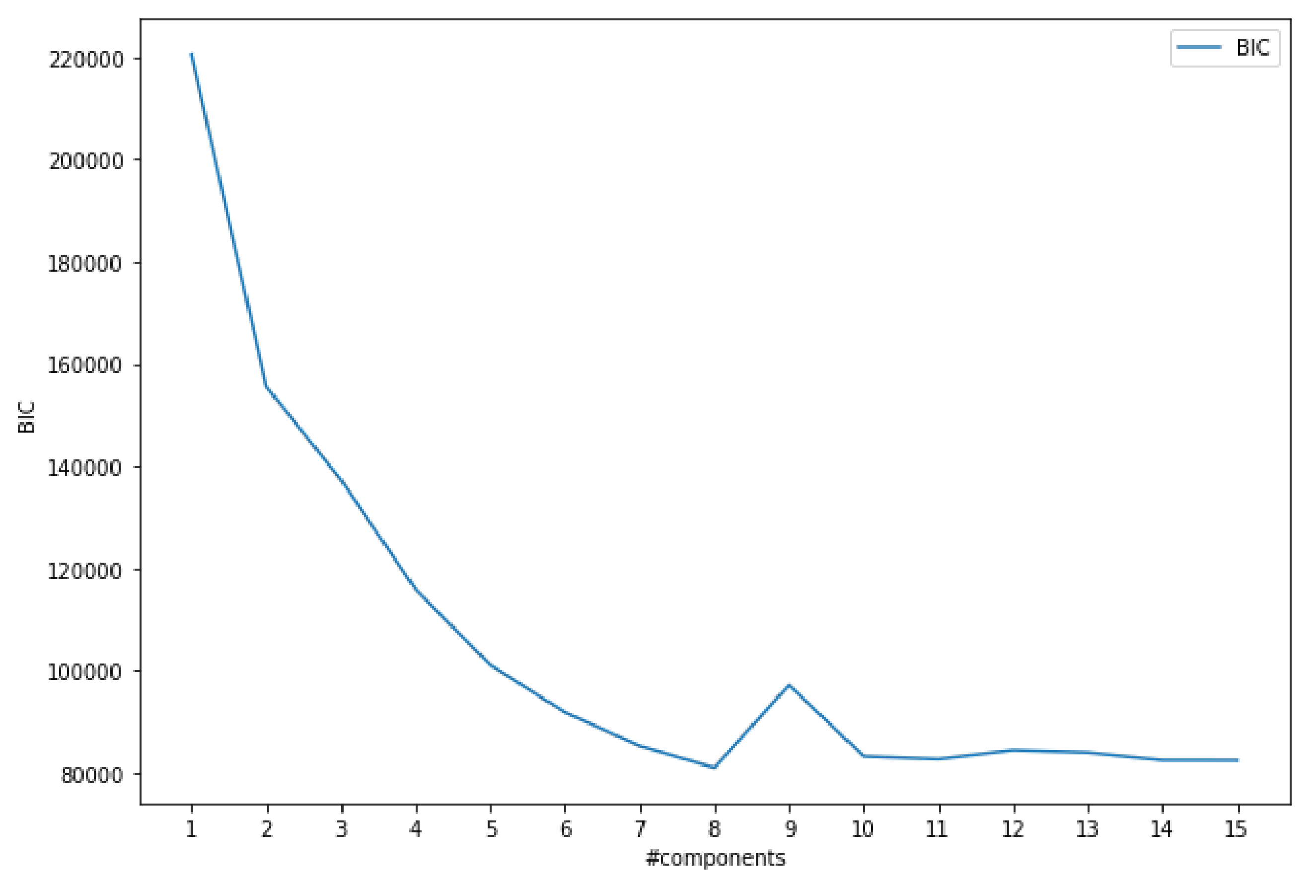
5.2. Bayesian Information Criterion

The Bayesian Information Criterion (BIC) is a useful metric for choosing between two or more alternative models [31]. Since we are modeling the data using a set of Gaussian models, BIC is used to determine the optimal number of components to characterize the set of time series. Given a dataset and a candidate model, BIC works by computing the logarithm of the likelihood of this model considering the set of likelihood-maximizing parameters θ ^ (for GMM, a set with k pairs ( μ ; σ )); it also penalizes the model proportionally to the number of parameters (for GMM, the number of components), so to reduce the chances of overfitting—refer to Equation (3).
B I C = 2 l o g ( L ( θ ^ ) ) + k l o g ( n )
where n is the number of samples; k is the number of components to test (we ranged from 1 through 15); L ( θ ^ ) is the likelihood of the model, with θ ^ as the parameter values that maximize the likelihood function.
Figure 6 depicts the value of metric BIC considering 1 through 15 Gaussian components. We verified that using eight components, the fitting of the model, discounted the overfitting penalization, reaches an optimal minimum value.

5.3. Further Supporting Statistics

From the Bayesian Information Criterion, we decided to use eight components. For comparison to other possible values, we present additional statistics as recommended by [39,40]; for comparison, we consider from 1 through 8 possible components, demonstrating that the higher the number of components, the better is the model fitting according to all the measurements. In Table 1, we present measurements of Log-likelihood (LL), computed for each of the n-components model; Aikake Information Criterion (AIC), based on the log-likelihood penalized by the number of parameters; Approximate Weight of Evidence (AWE) [41], an extension of the maximum likelihood criterion that takes the role of the features into account for each component; Consistent Aikake Information Criterion (CAIC), the same as AIC but adjusted by the sample size; Kullback Information Criterion (KIC) [42], the asymptotically unbiased estimator of the Kullback symmetric divergence measure; Sample Size-adjusted Bayesian Information Criterion (SABIC) [43], similar to BIC but adjusted by the sample size; and Integrated Completed Likelihood (ICL) [44], a version of BIC with improved arithmetic that more precisely approximate the integral part of the computation. All the metrics, but LL and ICL, indicate that the model is better adequate in accordance with how small the computed value is. For this analysis, we used R package tidyLPA [40].

5.4. Gaussian Components

In Table 2, one can see the numerical properties of each Gaussian component considering each of the 30-day snippets that originated it. We sorted each component by ratio average/standard_deviation in ascending order; as a result, the components whose elements have a higher number of hours and higher regularity have a higher rank. This order is fundamental to hour analysis as it carries a semantic characterization of the patients’ behavior.
According to our modeling, refer to Table 2 and Figure 7, ideally, every 30-day period of a patient should be characterized by components 7 (Ideal) or 8 (Plain), with several hours close to 7 h/night or above 8 h/night and a standard deviation of nearly just 1 h. Component 6 (Good) also corresponds to a high adherence, with a time of use above 7 h/night, but with a high standard deviation of +/−1.75 h. Component 5 (Highly adapted) indicates periods in which the patient is using the equipment regularly but with room for improvements in the number of hours. Components 4 Adapted is similar to component 5, but with a high instability of +/−2 h. Component 3 Pre-adaptation refers to periods of increasing adaptation, with an average below 5 h/night. However, components 1 Struggling and 2 Unstable refer to periods characterized by failure in using the equipment, with either a very low number of hours or a very high standard deviation, respectively. This classification takes into account the work of [21], who states that a minimum of 4 h/night is necessary for CPAP to be effective; and the work of [45], who verified that the prevalence of sleepiness, around 8.7%, is lower when the CPAP use lasts for more than 6 h/night if compared to patients who use the device for less than 4 h/night, presenting around 18.5% of sleepiness.
In Figure 7, we plot the eight Gaussian components of our model along with the corresponding instances of each one. In the center of each plot, one can see the mean series (prototype of the Gaussian component) along with the standard deviation and the standard deviation times two. The Gaussian nature is visually plausible.

5.5. LDA-Based Visualization

In Figure 8, we present a visual description of the snippets space colored according to the eight components detected via Gaussian Mixture Modeling. The figure is an instance of the method Linear Discriminant Analysis (LDA) [46], used to project the CPAP use dataset onto a 3-dimensional space. LDA, similar to Principal Component Analysis, finds the component axes that maximize the variance of the data at the same time that it sets axes to maximize the separation between classes. The plot illustrates the set of series as a whole with non-evident gaps nor low-density regions, but for the outliers. The use of GMM allowed the partitioning of the space in a way that density-oriented hard clustering methods failed.

5.6. GMM-Based Patient Characterization

So far, we have focused on characterizing periods of 30-days of CPAP use. This is because of our assumption that the regime of use of the equipment varies over time: at the beginning of the therapy; after years of use; during a period of stress, possibly accompanied by insomnia [25]; while treating another infirmity; and so on, i.e., characterizing an entire series of use would not be precisely informative, but yet, analyzing such a historical series is necessary, as the doctor needs to understand the evolution of the therapy and detected periods of low efficacy.
For the task of characterizing the entire record of CPAP use of a given patient, we propose to apply our proposed GMM analysis by means of the classic sliding-window method. Therefore, for a time series with n time-stamped signals, we consider the i-th signal and the following 29 signals, forming a window with 30 signals. We iterate over i, 1 i n 30 , in a total of n 30 steps. For each iteration, we fit the 30-signals window in our model to obtain a status number ranging from 1 through 8, corresponding to one of our possible GMM characterizations. The result is a time series in which every point indicates the 30-days status of the patient at any given time, as illustrated in Figure 9. In Figure 9a, one can observe the historical CPAP use of a patient for 370 days; Figure 9c presents the corresponding GMM characterization, which summarizes the behavior of the patient in a time series in which the periods of high and low adherence become more explicit. In Figure 9b, we see a patient with 1603 recordings of CPAP use; the corresponding GMM analysis is presented in Figure 9d. In this second example, the simplification of the data and the sharper characterization of the adherence become even more evident.

6. Discussion

In comparison to former works, as reviewed in the related works, one strong point of our methodology is that we do not assume the patient to be a static entity, which might distort the interpretation of the actual state of a patient. In the work of [22], for example, the patient characterization will not correspond to its latest months of CPAP use but, rather, to the most prominent patterns of use as observed in her/his, say, two years of use, i.e., a given patient might be referred to as being fully adapted to using the equipment when she/he just started to struggle in carrying out the therapy due to external factors that took place in recent times, causing prejudice to the proper evaluation of adherence. We also exceed in introducing a more granular 8-classes characterization statistically and visually verified; since each of our components encompassed a set of 30-day series with distinct and similar numerical properties, as demonstrated in Section 5, we advocate that the proposed cluster-based characterization is more comprehensive than that of previous works. This allegation is supported by ample statistics and by our set of extracted snippets, which has a cardinality larger than that of any dataset used in the similar analysis that we reviewed; that is, we count on a strong support to our findings.
Another advance of our methodology is that we do not resort to aggregation to simplify the analysis of a given patient’s series. This way, we avoid the loss of information due to aggregation [15,16] and the misconception of providing a number holding no referential to the most usual 30-day-long patterns found in a real database. For example, if one verifies that the average of a patient’s series is 5 h/night, it is possible that the physician will consider the patient to have high adherence to the treatment, which makes sense from an initial perspective. However, if we take the classes’ average and standard deviation presented in Table 2, it is possible that this patient is behaving in any one of classes 1 through 5, i.e., by considering a real clinical database, we found out that the average of a time series can lead to a total misconception of what is really happening.
Furthermore, from our investigation and by inspecting the state of the art, we verified that there is no agreement with respect to the number of characterizations (cluster/classes) of patients in the field of OSA and CPAP therapy. As reported in the related works, existing works report from four up to seven classes, diverging even for the same research team over different datasets [22,24]. This variability, while not desired, does not invalidate the investigations carried out; nevertheless, it is evidence that there is not a definitive answer to the problem of cluster-based patient characterization. Possibly, this variability comes from peculiarities of the cohort being studied to the specific variable considered under each methodology, algorithmic traits, and even different interpretations of the results. As a result, one conclusion of ours is that the methodologies are more relevant than the presented results; and that each context in which they are to be employed must perform specific cluster analysis in accordance with the data nature and the needs of the analytic application. Regardless, the state of the art reinforces the importance and impact of research in ACPA monitoring and adherence, which ranges from preventing or working towards the prevention of cardiovascular diseases [47] to the study of improving neurocognitive response through OSA treatment [48]. Thus, our work sets new pathways for research on ACPA and OSA, directing further investigation with techniques beyond Gaussian mixture modeling in future works.

7. Conclusions

We introduced an unsupervised machine-learning methodology based on a Gaussian Mixture Modeling (GMM) employed over a set of recurrent 30-day-long patterns (snippets) extracted from a database of CPAP use time series. We tested our methodology over a dataset provided by a French hospital that collects CPAP telemonitored data (hours of use per night) regarding over 2000 patients. As a result, we identified eight characteristic patient behaviors regarding CPAP use adherence as indicated by the GMM components. This procedure demonstrated success in classifying any 30-day-long period of CPAP use according to a frame of eight classes that progressively indicate more efficient adherence.
Our approach is an alternative to the usually employed average-based aggregations, which can potentially lose important information, and that provide a number holding no referential magnitude to permit a proper interpretation. In addition, we demonstrated the use of our GMM-based classification combined with the classic method of sliding window; by considering 30-day-long periods, it becomes possible to simplify the entire time series of a given patient, providing less information but more promptly understandable patient behavior. Along with this investigation, we also collected evidence that, in the field of OSA and CPAP therapy, there is not a consensus on the number of classes to which the patients correspond, indicating that such unsupervised machine-learning analyses must pass through a new data fitting whenever the dataset or goals change significantly.
We expect our contributions to support physicians in more precisely evaluating the adherence of patients to the CPAP therapy. This might take place as a computer-aided diagnosis system or as full-time monitoring that issues alarms when critical situations are detected. Such a monitoring system is highly needed as telemonitored equipment produces larger and larger data streams overcoming the capacity of physicians to timely inspect the conditions of the patients. As a last remark, we suggest that future work is to employ our methodology over other attributes produced during the treatment of OSA, mainly the Apnea–Hypopnea Index.

Author Contributions

Conceptualization, J.F.R.J., S.B., J.-L.P., G.S. and L.G.; methodology, J.F.R.J. and S.A.-Y.; software, J.F.R.J.; validation, G.S., S.B., J.-L.P. and L.G.; formal analysis, J.F.R.J.; investigation, J.F.R.J.; resources, S.A.-Y.; data curation, S.B., J.-L.P., L.G. and G.S.; writing—original draft preparation, J.F.R.J.; writing—review and editing, S.B., J.-L.P., L.G., G.S. and S.A.-Y.; visualization, J.F.R.J.; supervision, S.A.-Y.; project administration, J.F.R.J.; funding acquisition, S.A.-Y. All authors have read and agreed to the published version of the manuscript.

Funding

This research was partially financed by the French agency Multidisciplinary Institute in Artificial Intelligence MIAI - Grenoble Alpes (Grant ANR-19-P3IA0003) and the “e-health and integrated care” Chair of excellence from the Grenoble Alpes University Foundation and the French National Research Agency in the framework of the Investissements d’Avenir program (Grant ANR-15-IDEX-02); by the Canada First Research Excellence Fund (CFREF) through the Ocean Frontier Institute (OFI) at Dalhousie University, Halifax - NS, Canada; and by Brazilian agencies Fundação de Amparo à Pesquisa do Estado de São Paulo (2019/04461-9, 2018/17620-5, 2017/08376-0, and 2016/17078-0); Conselho Nacional de Desenvolvimento Cientifico e Tecnologico (167967/2017-7, 305580/2017-5, 406550/2018-2, and 307946/2021-5); and Coordenacao de Aperfeicoamento de Pessoal de Nivel Superior (CAPES, Finance Code 001).

Data Availability Statement

The data used for the experiment is private and cannot be made available to the public due to privacy reasons. However, the neural network models produced during experiments are publicly available.

Conflicts of Interest

The authors declare no conflict of interest.

References

  1. Franco, P.; Bourdin, H.; Braun, F.; Briffod, J.; Pin, I.; Challamel, M.J. Diagnostic du syndrome d’apnée obstructive du sommeil chez l’enfant (2–18 ans): Place de la polysomnographie et de la polygraphie ventilatoire. Syndrome d’apnée obstructive du sommeil de l’enfant (SAOS) Recommandations de la Société Française de Recherche et Médecine du Sommeil. Arch. PéDiatrie 2017, 24, S16–S27. [Google Scholar] [CrossRef] [PubMed]
  2. Benjafield, A.V.; Ayas, N.T.; Eastwood, P.R.; Heinzer, R.; Ip, M.S.; Morrell, M.J.; Nunez, C.M.; Patel, S.R.; Penzel, T.; Pepin, J.L. Estimation of the global prevalence and burden of obstructive sleep apnoea: A literature-based analysis. Lancet Respir. Med. 2019, 7, 687–698. [Google Scholar] [CrossRef] [Green Version]
  3. Watson, N.F. Health Care Savings: The Economic Value of Diagnostic and Therapeutic Care for Obstructive Sleep Apnea. J. Clin. Sleep Med. 2016, 12, 1075–1077. [Google Scholar] [CrossRef] [PubMed] [Green Version]
  4. Gilat, H.; Vinker, S.; Buda, I.; Soudry, E.; Shani, M.; Bachar, G. Obstructive sleep apnea and cardiovascular comorbidities: A large epidemiologic study. Medicine 2014, 93, e45. [Google Scholar] [CrossRef] [PubMed]
  5. DiMatteo, M.R. Variations in patients’ adherence to medical recommendations: A quantitative review of 50 years of research. Med. Care 2004, 42, 200–209. [Google Scholar] [CrossRef] [PubMed]
  6. Iannella, G.; Lechien, J.R.; Perrone, T.; Meccariello, G.; Cammaroto, G.; Cannavicci, A.; Burgio, L.; Maniaci, A.; Cocuzza, S.; Di Luca, M.; et al. Barbed reposition pharyngoplasty (BRP) in obstructive sleep apnea treatment: State of the art. Am. J. Otolaryngol. 2022, 43, 103197. [Google Scholar] [CrossRef]
  7. Wang, D.; Tang, Y.; Chen, Y.; Zhang, S.; Ma, D.; Luo, Y.; Li, S.; Su, X.; Wang, X.; Liu, C.; et al. The effect of non-benzodiazepine sedative hypnotics on CPAP adherence in patients with OSA: A systematic review and meta-analysis. Sleep 2021, 44, zsab077. [Google Scholar] [CrossRef]
  8. Engleman, H.M.; Wild, M.R. Improving CPAP use by patients with the sleep apnoea/hypopnoea syndrome (SAHS). Sleep Med. Rev. 2003, 7, 81–99. [Google Scholar] [CrossRef]
  9. Pépin, J.L.; Tamisier, R.; Hwang, D.; Mereddy, S.; Parthasarathy, S. Does remote monitoring change OSA management and CPAP adherence? Respirology 2017, 22, 1508–1517. [Google Scholar] [CrossRef]
  10. Varma, N.; Ricci, R.P. Telemedicine and cardiac implants: What is the benefit? Eur. Heart J. 2013, 34, 1885–1895. [Google Scholar] [CrossRef] [Green Version]
  11. Mendelson, M.; Vivodtzev, I.; Tamisier, R.; Laplaud, D.; Dias-Domingos, S.; Baguet, J.P.; Moreau, L.; Koltes, C.; Chavez, L.; De Lamberterie, G.; et al. CPAP treatment supported by telemedicine does not improve blood pressure in high cardiovascular risk OSA patients: A randomized, controlled trial. Sleep 2014, 37, 1863–1870. [Google Scholar] [CrossRef]
  12. Chang, J.; Derose, S.; Benjafield, A.; Crocker, M.; Kim, J.; Becker, K.; Woodrum, R.; Arguelles, J.; Hwang, D. Acceptance and Impact of Telemedicine in Patient Sub-Groups with Obstructive Sleep Apnea: Analysis from the Tele-Osa Randomized Clinical Trial; Sleep. Oxford University Press Inc. Journals Dept.: Cary, NC, USA, 2017; Volume 40, pp. A201–A202. [Google Scholar]
  13. Stepnowsky, C.; Palau, J.; Marler, M.; Gifford, A. Pilot randomized trial of the effect of wireless telemonitoring on compliance and treatment efficacy in obstructive sleep apnea. J. Med. Internet Res. 2007, 9, e14. [Google Scholar] [CrossRef]
  14. Stepnowsky, C.J.; Marler, M.R.; Ancoli-Israel, S. Determinants of nasal CPAP compliance. Sleep Med. 2002, 3, 239–247. [Google Scholar] [CrossRef]
  15. McKee, G.J.; Miljkovic, D. Data Aggregation and Information Loss; Technical Report 9843; American Agricultural Economics Association: Ames, IA, USA, 2007. [Google Scholar]
  16. Orcutt, G.H.; Watts, H.W.; Edwards, J.B. Data Aggregation and Information Loss. Am. Econ. Rev. 1968, 58, 773–787. [Google Scholar]
  17. Ye, L.; Pien, G.W.; Ratcliffe, S.J.; Björnsdottir, E.; Arnardottir, E.S.; Pack, A.I.; Benediktsdottir, B.; Gislason, T. The different clinical faces of obstructive sleep apnoea: A cluster analysis. Eur. Respir. J. 2014, 44, 1600–1607. [Google Scholar] [CrossRef] [Green Version]
  18. Gagnadoux, F.; Le Vaillant, M.; Paris, A.; Pigeanne, T.; Leclair-Visonneau, L.; Bizieux-Thaminy, A.; Alizon, C.; Humeau, M.P.; Nguyen, X.L.; Rouault, B. Relationship between OSA clinical phenotypes and CPAP treatment outcomes. Chest 2016, 149, 288–290. [Google Scholar] [CrossRef] [Green Version]
  19. Bailly, S.; Destors, M.; Grillet, Y.; Richard, P.; Stach, B.; Vivodtzev, I.; Timsit, J.F.; Lévy, P.; Tamisier, R.; Pépin, J.L.; et al. Obstructive sleep apnea: A cluster analysis at time of diagnosis. PLoS ONE 2016, 11, e0157318. [Google Scholar] [CrossRef] [Green Version]
  20. Subramani, Y.; Singh, M.; Wong, J.; Kushida, C.A.; Malhotra, A.; Chung, F. Understanding phenotypes of obstructive sleep apnea: Applications in anesthesia, surgery, and perioperative medicine. Anesth. Analg. 2017, 124, 179. [Google Scholar] [CrossRef]
  21. Smith, I.; Lasserson, T.; Haniffa, M. Interventions to improve use of continuous positive airway pressure for obstructive sleep apnoea. Cochrane Database Syst. Rev. 2004, 18. [Google Scholar] [CrossRef]
  22. Babbin, S.F.; Velicer, W.F.; Aloia, M.S.; Kushida, C.A. Identifying longitudinal patterns for individuals and subgroups: An example with adherence to treatment for obstructive sleep apnea. Multivar. Behav. Res. 2015, 50, 91–108. [Google Scholar] [CrossRef]
  23. Hoeppner, B.B.; Goodwin, M.S.; Velicer, W.F.; Mooney, M.E.; Hatsukami, D.K. Detecting longitudinal patterns of daily smoking following drastic cigarette reduction. Addict. Behav. 2008, 33, 623–639. [Google Scholar] [CrossRef] [Green Version]
  24. Aloia, M.S.; Goodwin, M.S.; Velicer, W.F.; Arnedt, J.T.; Zimmerman, M.; Skrekas, J.; Harris, S.; Millman, R.P. Time series analysis of treatment adherence patterns in individuals with obstructive sleep apnea. Ann. Behav. Med. 2008, 36, 44–53. [Google Scholar] [CrossRef]
  25. Drake, C.L.; Roehrs, T.; Roth, T. Insomnia causes, consequences, and therapeutics: An overview. Depress. Anxiety 2003, 18, 163–176. [Google Scholar] [CrossRef]
  26. Imani, S.; Madrid, F.; Ding, W.; Crouter, S.; Keogh, E. Matrix Profile XIII: Time Series Snippets: A New Primitive for Time Series Data Mining. In Proceedings of the 2018 IEEE International Conference on Big Knowledge (ICBK), Singapore, 17–18 November 2018; pp. 382–389. [Google Scholar]
  27. Gharghabi, S.; Imani, S.; Bagnall, A.; Darvishzadeh, A.; Keogh, E. An Ultra-Fast Time Series Distance Measure to Allow Data Mining in More Complex Real-World Deployments; Springer: Berlin/Heidelberg, Germany, 2018. [Google Scholar]
  28. Barandas, M.; Folgado, D.; Fernandes, L.; Santos, S.; Abreu, M.; Bota, P.; Liu, H.; Schultz, T.; Gamboa, H. TSFEL: Time Series Feature Extraction Library. SoftwareX 2020, 11, 100456. [Google Scholar] [CrossRef]
  29. Taskesen, E. pca. 2019. Available online: https://github.com/erdogant/pca (accessed on 21 April 2022).
  30. Lohninger, H. Fundamentals of Statistics; Epina Bookshelf; Harvard University Press: Cambridge, MA, USA, 2010; Volume 5. [Google Scholar]
  31. Fabozzi, F.J.; Focardi, S.M.; Rachev, S.T.; Arshanapalli, B.G. The Basics of Financial Econometrics: Tools, Concepts, and Asset Management Applications; John Wiley & Sons: Hoboken, NJ, USA, 2014. [Google Scholar]
  32. Reynolds, D.A. Gaussian Mixture Models. Encycl. Biom. 2009, 741, 659–663. [Google Scholar]
  33. Povinelli, R.J.; Johnson, M.T.; Lindgren, A.C.; Ye, J. Time series classification using Gaussian mixture models of reconstructed phase spaces. IEEE Trans. Knowl. Data Eng. 2004, 16, 779–783. [Google Scholar] [CrossRef] [Green Version]
  34. Eirola, E.; Lendasse, A. Gaussian mixture models for time series modelling, forecasting, and interpolation. In International Symposium on Intelligent Data Analysis; Springer: Berlin/Heidelberg, Germany, 2013; pp. 162–173. [Google Scholar]
  35. Krishnan Nair, K.; Kiremidjian, A.S. Time Series Based Structural Damage Detection Algorithm Using Gaussian Mixtures Modeling. J. Dyn. Syst. Meas. Control 2006, 129, 285–293. [Google Scholar] [CrossRef]
  36. Reddy, A.; Ordway-West, M.; Lee, M.; Dugan, M.; Whitney, J.; Kahana, R.; Ford, B.; Muedsam, J.; Henslee, A.; Rao, M. Using Gaussian Mixture Models to Detect Outliers in Seasonal Univariate Network Traffic. In Proceedings of the 2017 IEEE Security and Privacy Workshops (SPW), San Jose, CA, USA, 25 May 2017; pp. 229–234. [Google Scholar]
  37. Le, T.Q.; Cheng, C.; Sangasoongsong, A.; Bukkapatnam, S.T.S. Prediction of sleep apnea episodes from a wireless wearable multisensor suite. In Proceedings of the 2013 IEEE Point-of-Care Healthcare Technologies (PHT), Bangalore, India, 16–18 January 2013; pp. 152–155. [Google Scholar]
  38. MacQueen, J. Some methods for classification and analysis of multivariate observations. In Proceedings of the Fifth Berkeley Symposium on Mathematical Statistics and Probability, Oakland, CA, USA, 21 June 1967; Volume 1, pp. 281–297. [Google Scholar]
  39. Akogul, S.; Erisoglu, M. A Comparison of Information Criteria in Clustering Based on Mixture of Multivariate Normal Distributions. Math. Comput. Appl. 2016, 21, 34. [Google Scholar] [CrossRef] [Green Version]
  40. Rosenberg, J.M.; Beymer, P.N.; Anderson, D.J.; van Lissa, C.; Schmidt, J.A. tidyLPA: An R Package to Easily Carry Out Latent Profile Analysis (LPA) Using Open-Source or Commercial Software. J. Open Source Softw. 2018, 3, 978. [Google Scholar] [CrossRef] [Green Version]
  41. Banfield, J.D.; Raftery, A.E. Model-Based Gaussian and Non-Gaussian Clustering. Biometrics 1993, 49, 803–821. [Google Scholar] [CrossRef]
  42. Seghouane, A.K.; Bekara, M. A small sample model selection criterion based on Kullback’s symmetric divergence. IEEE Trans. Signal Process. 2004, 52, 3314–3323. [Google Scholar] [CrossRef]
  43. Sclove, S.L. Application of model-selection criteria to some problems in multivariate analysis. Psychometrika 1987, 52, 333–343. [Google Scholar] [CrossRef]
  44. Biernacki, C.; Celeux, G.; Govaert, G. Assessing a Mixture Model for Clustering with the Integrated Classification Likelihood. IEEE Trans. Pattern Anal. Mach. Intell.—PAMI 1997, 22, 719–725. [Google Scholar] [CrossRef]
  45. Gasa, M.; Tamisier, R.; Launois, S.H.; Sapene, M.; Martin, F.; Stach, B.; Grillet, Y.; Levy, P.; Pepin, J.L. Residual sleepiness in sleep apnea patients treated by continuous positive airway pressure. J. Sleep Res. 2013, 22, 389–397. [Google Scholar] [CrossRef]
  46. Balakrishnama, S.; Ganapathiraju, A. Linear Discriminant Analysis—A Brief Tutorial. Inst. Signal Inf. Process. 1998, 18, 1–8. [Google Scholar]
  47. Pollicina, I.; Maniaci, A.; Lechien, J.R.; Iannella, G.; Vicini, C.; Cammaroto, G.; Cannavicci, A.; Magliulo, G.; Pace, A.; Cocuzza, S.; et al. Neurocognitive Performance Improvement after Obstructive Sleep Apnea Treatment: State of the Art. Behav. Sci. 2021, 11, 180. [Google Scholar] [CrossRef]
  48. Yeghiazarians, Y.; Jneid, H.; Tietjens, J.R.; Redline, S.; Brown, D.L.; El-Sherif, N.; Mehra, R.; Bozkurt, B.; Ndumele, C.E.; Somers, V.K.; et al. Obstructive Sleep Apnea and Cardiovascular Disease: A Scientific Statement From the American Heart Association. Circulation 2021, 144, e56–e67. [Google Scholar] [CrossRef]
Figure 1. Sample of a CPAP use time series obtained by means of telemonitoring. One-year-long times series of CPAP use (#hours) of a real anonymized patient. The number of hours ranges from 0 (the patient did not use, or was not able to use the CPAP) up to 10 h of use.
Applsci 12 07618 g001
Figure 2. Basic distributions related to the CPAP use dataset. (a) Distribution of the length of the time series (number of days of use) found in the CPAP use dataset. We discarded patients with less than 181 days (6 months) of monitoring. (b) Distribution of the average number of hours of CPAP use considering all the patients with, at least, 181 days of monitoring.
Applsci 12 07618 g002
Figure 3. Our methodology to characterize the periods of CPAP use based on analytical techniques over a real-world dataset.
Applsci 12 07618 g003
Figure 4. Example of a time series with two detected snippets along with the main matches of each one. By exact match, we mean the snippet has maximum MPdist similarity to a subsequence in the original time series; a partial match means the similarity is high but not maximal.
Applsci 12 07618 g004
Figure 5. Visualization of the two components that explain 99% of variance as identified by method Principal Component Analysis.
Applsci 12 07618 g005
Figure 6. Bayesian Information Criterion test for the number of Gaussian models that fit our data.
Applsci 12 07618 g006
Figure 7. Time series plot of the eight components that characterize the CPAP use 30-days snippets extracted from the CPAP use dataset. Each plot presents the mean (thickest red line), the variance, and two times the variance lines. Notice that we present the average because it is a parameter to the Gaussian distribution; we do not depend on this computation to characterize the time series.
Applsci 12 07618 g007
Figure 8. Plot 3D using technique Linear Discriminant Analysis applied over the 30-days summarization snippets.
Applsci 12 07618 g008
Figure 9. GMM characterization of two patients from the CPAP use dataset. The first patient in plot (a) and its corresponding sliding-window characterization in plot (c). The second patient in plot (b) characterized in plot (d).
Applsci 12 07618 g009
Table 1. Additional statistics Log-likelihood (LL), Aikake Information Criterion (AIC), Approximate Weight of Evidence (AWE) [41], Consistent Aikake Information Criterion (CAIC), Kullback Information Criterion (KIC) [42], Sample Size-adjusted Bayesian Information Criterion (SABIC) [43], and Integrated Completed Likelihood (ICL) [44].
#CompsLLAICAWECAICKICSABICICL
1−331,566663,173663,594663,355663,196663,271−663,335
2−323,953647,988648,855648,361648,032648,189−654,536
3−319,721639,567640,878640,130639,632639,871−648,605
4−318,231636,627638,383637,381636,713637,035−649,319
5−317,349634,907637,108635,852635,014635,417−650,038
6−316,502633,254635,899634,390633,382633,867−650,552
7−315,985632,261635,351633,588632,410632,978−650,243
8−315,801631,936635,470633,453632,106632,756−653,016
Table 2. Summary of the properties of each of the eight components, including percentage of the snippets in each component, average h/night along with standard deviation and standard deviation*2, energy (summation of the average signal). The order of the components is given by ratio average*1/standard_deviation; that is, the higher in the rank the more hours of use and more regularity (lower standard deviation).
Comp% Elementsavg
(h/Night)
stdstd*2Energyavg/stdStatus
16.85%3.691.643.29110.612.24Struggling
27.30%6.873.026.05206.172.27Unstable
38.29%4.851.693.37145.632.88Pre-adaptation
417.51%6.211.963.93186.203.16Adapted
513.76%5.561.472.94166.823.79Highly adapted
613.15%7.901.753.50236.904.52Good
720.68%7.071.052.10212.106.72Ideal
812.46%8.551.142.27256.547.52Plain
Publisher’s Note: MDPI stays neutral with regard to jurisdictional claims in published maps and institutional affiliations.

