Questioning the Anisotropy of Pedestrian Dynamics: An Empirical Analysis with Artificial Neural Networks

Abstract

Identifying the factors that control the dynamics of pedestrians is a crucial step towards modeling and building various pedestrian-oriented simulation systems. In this article, we empirically explore the influential factors that control the single-file movement of pedestrians and their impact. Our goal in this context is to apply feed-forward neural networks to predict and understand the individual speeds for different densities of pedestrians. With artificial neural networks, we can approximate the fitting function that describes pedestrians’ movement without having modeling bias. Our analysis is focused on the distances and range of interactions across neighboring pedestrians. As indicated by previous research, we find that the speed of pedestrians depends on the distance to the predecessor. Yet, in contrast to classical purely anisotropic approaches—which are based on vision fields and assume that the interaction mainly depends on the distance in front—our results demonstrate that the distance to the follower also significantly influences movement. Using the distance to the follower combined with the subject pedestrian’s headway distance to predict the speed improves the estimation by 18% compared to the prediction using the space in front alone.

1. Introduction

For the sake of safe mass events, comfortable and efficient transport infrastructures, for example, airports, much work is dedicated to understanding the laws governing crowd dynamics. In recent years, the number of empirical studies increased significantly, which led to more insights into the movement of people. Additionally, these insights often offer useful criteria that validate models and evaluate the simulacrum of reality they create.

Trustworthy models are valuable tools that shed light on unknown aspects of crowds and allow for assessing and investigating new design and planning measures. However, most known modeling approaches make implicit assumptions on the way people move and interact with their environment. Cellular automata, for instance, assume that a pedestrians’ motile behavior is determined by chemotaxis [1]. Another popular modeling ansatz describes the crowd by differential equations, assuming constructed functions such as algebraic [2] or exponential [3] Newtonian forces compactly describe a system’s evolution. It is worth noting that in [4], the interaction energy between pedestrians was measured from field observations and not assumed.

Based solely on experimental evidence, in this work, we isolate the factors that influence the interactions between pedestrians in single-file movement. Contrary to the usual synergy between experimental and numerical investigations of pedestrian dynamics, where the former validates the latter, we try, through neural networks, to “extract” from empirical data the most relevant dependencies that determine the movement of pedestrians. Furthermore, classical pedestrian interaction models are anisotropic, assuming that people in front influence the dynamics more than people behind. For instance, most force-based models include vision field mechanisms affecting a weight depending on the bearing angle in the motion direction [2,3,5,6]. This hypothesis, despite the reasonable limits of human perception and notions of fields of vision, is in most cases assumed a priori without statistical evidence. In this article, we analyze the interaction range in single-file movement, including isotropic symmetric interaction models based on the distance to pedestrians behind as well. Recently, artificial neural networks have been used successfully to estimate the speed of pedestrians in different complex geometries [7]. They allow identifying (with no modeling bias) which variables are relevant to the pedestrian by analyzing prediction errors. In this context, we investigate several factors influencing the dynamics, namely the interaction range with pedestrians in front and behind, and the isotropic nature of the pedestrian dynamics. Hereby, we focus our analysis on the influence of the distance to the follower, predecessor, and second predecessor pedestrian on the prediction of the subject pedestrian speed.

The rest of this article is organized as follows. In Section 2, we review and discuss several approaches proposed by researchers to predict pedestrians’ movement characteristics using different methods and techniques. In Section 3, the single-file movement experimental dataset is introduced, and the data pre-processing methodology is described. Section 4 presents the structure of the artificial neural networks applied to investigate pedestrians’ movement influential factors to predict future speeds. In Section 5, the speed prediction results using different input features are discussed. Finally, we summarize the article, make conclusions, and propose future work in Section 6.

2. Related Work

Recently, more attention has been given to studying the influential factors that control the dynamics of pedestrians in closed and open environments [8,9,10,11,12,13]. Understanding such factors can help in modeling complex pedestrian movement. When dealing with complex systems, such as pedestrian dynamics, scientists generate numerous models based on different approaches, variables, and parameters [14]. For instance, force-based models (see [15] for a review) assume that pedestrians’ deviation from their intended trajectories can be explained by external forces. Another ansatz by Karamouzas et al. [4] follows a statistical–mechanical approach to measure the interaction energy between pedestrians based on the time to a potential future collision (time-to-collision). Tordeux et al. [16] introduce the walking time-gap as a parameter to model pedestrian movement. Van den Berg et al. [17] propose a model based on optimal collision-avoidance techniques to describe the movement of pedestrians in two-dimensional space. Another model, the Linear Trajectory Avoidance (LTA) model, introduced by Pellegrini et al. [18], takes into account both simple scene information in the form of destinations or desired directions and interactions between different pedestrians. Cellular automaton model proposed by Schadschneider et al. [1] is inspired by the chemotaxis process, which ants use for communication. This discrete on-space model assumes that pedestrian transition to neighbor cell probability varies dynamically and is not constant. Thus, this model modifies the transition probabilities by considering the nearest-neighbor interactions to determine pedestrian’s transition to the next state. The aforementioned classical models are anisotropic, i.e., they assume that pedestrians interact with people in their vision field, and this interaction is reduced with the people behind. For instance, most force-based models include a vision field affecting a weight depending on the bearing angle ${\theta }_{ij}$ [2,3,5,6]. In the centrifugal and generalized centrifugal force model [2,6], the weight is

$${\omega }_1\left({\theta }_{ij}\right)=\left\{\begin{array}{cc}cos\left({\theta }_{ij}\right)\hfill & \mathrm{if}|{\theta }_{ij}|<\pi /2\hfill \\ 0\hfill & \mathrm{otherwise}\hfill \end{array}\right.$$

(1)

In the original social force model [3], the weight is

$${\omega }_2\left({\theta }_{ij}\right)=\left\{\begin{array}{cc}1\hfill & \mathrm{if}|{\theta }_{ij}|<\phi \hfill \\ c\hfill & \mathrm{otherwise}\hfill \end{array}\right.$$

(2)

where $\phi$ is the angle of sight, and $0<c<1$ is a reduced perception factor. Extended social force models use the weight [5]

$${\omega }_3\left({\theta }_{ij}\right)={\lambda }_i+(1-{\lambda }_i)\frac{1+cos\left({\theta }_{ij}\right)}{2},{\lambda }_i\approx 0.75$$

(3)

Such mechanisms make the motion behavior highly anisotropic. For single-file motion, it may even induce the interaction model to be strictly anisotropic (i.e., depending solely on the distances in front). In this article, we analyze the interaction range in single-file movement, including isotropic symmetric interaction models based on the distance to pedestrians behind as well. Furthermore, all previously discussed models introduce equations that provide a template for a large but tightly linked family of models. However, sometimes the choice of certain qualitative functions is not justified, nor is it backed by empirical knowledge of pedestrian dynamics. Moreover, classical models have a bias that emerges from their form, which has restricted degrees of freedom. That means each model can be controlled by a few specific parameters inherent to the form of the model. The prediction quality usually depends on the pertinence of the model’s form defined to describe pedestrians’ movements.

Recently, many researchers have proposed human trajectory prediction algorithms [19], arguing that neural networks have high flexibility and are devoid of any modeling bias. For example, Alahi et al. [13] develop the Social LSTM (S-LSTM) algorithm to predict the future trajectories of pedestrians depending on their past positions and the interactions with their neighbors. To model the social interaction, Alahi uses a social-pooling layer to allow sharing each neighboring pedestrian’s LSTM hidden state to predict the subject pedestrian’s future positions. The Alahi et al. algorithm improved the prediction of the next position by a factor of approximately 21% compared to the force-based model (SF) [3]. Xue et al. [20] develop a trajectory-prediction algorithm, called the Bi-prediction algorithm, based on the S-LSTM and considering the importance of pedestrians’ intended destinations in predicting their future trajectories. This two-stage prediction model employs bidirectional LSTM architecture to forecast multiple possible trajectories with different probabilities in the scene. In other research [21], the authors propose the MX-LSTM model, which adds to the previous models a new variable (direction of the pedestrian head) to improve the trajectory predictions (the model improves the prediction by approximately 19% compared to the SF classical model). All the aforementioned data-based approaches have been used to describe low-density situations using specific datasets (UCY [22], ETH [18], etc.) where social interactions techniques for collision avoidance take up to several meters.

Other researchers have focused on developing algorithms based on artificial neural networks to predict a pedestrian’s speed. For instance, the study proposed by Tordeux et al. [7] applies feed-forward neural networks (FFNN) to predict the speed of pedestrians walking on different types of facilities (corridors and bottlenecks). Several FFNNs are presented to approximate the fitting function with different combinations of input features (relative positions, relative velocities, and mean distance to the nearest ten neighbors in front), hidden layers, and hidden neurons. The results of FFNN show improvement by $20\%$ compared to the classical approach (Weidmann fitting model [23]) evaluated with mixed data (corridor and bottleneck). In another study by Tkachuk et al. [24], the authors develop a system that simulates pedestrians’ behavior during the evacuation process. The proposed system uses FFNN to predict how people act during evacuations. The acceleration and average velocity are used to predict each pedestrian’s horizontal and vertical speeds. Another study by Yi Ma et al. [25] proposes an approach based on a multilayer perceptron artificial neural network for simulating pedestrians’ behavior. The authors train the artificial neural network using pedestrians’ actual movement data to encapsulate and predict their future behaviors. To verify the correctness of the proposed simulation system, the authors compared the simulation results of pedestrian counter-flow in a road-crossing situation and pedestrian collision avoidance with the actual experiments. The simulation results in both studies show that the proposed models based on artificial neural networks provide greater prediction accuracy by learning from actual experimental data rather than other models.

For brevity’s sake, our focus in this article is to apply a FFNN to investigate and analyze empirically the impact of distance interaction range on dynamics of pedestrians without modeling bias. Unlike most current research work, we aim to analyze single-file movement in different homogeneous and heterogeneous gender flows to predict the pedestrian’s speed.

3. Experimental Data and Measurement Methods

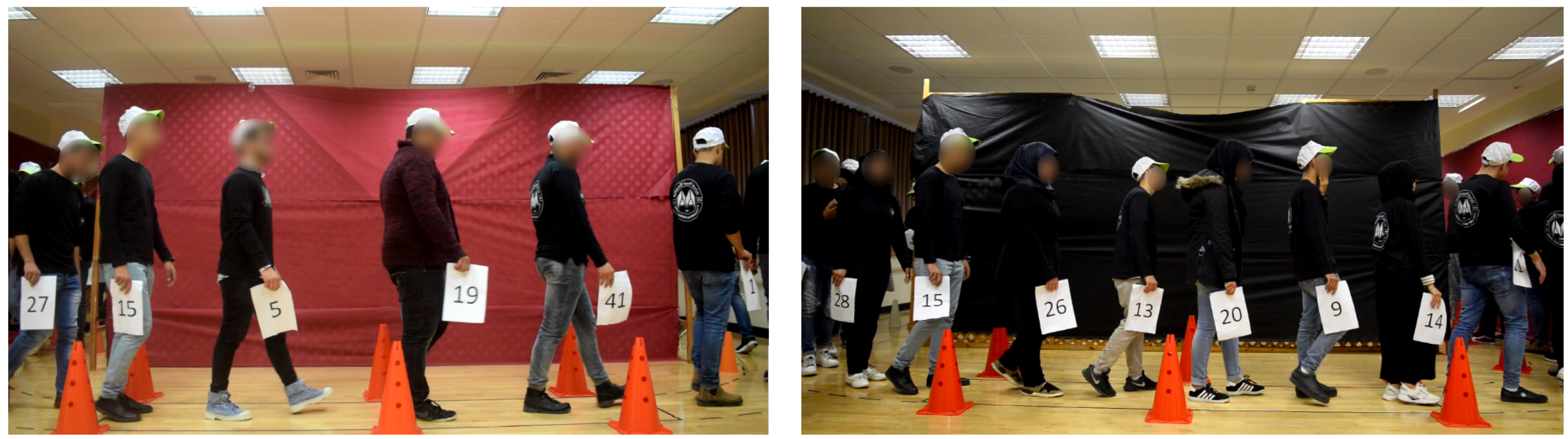
This section presents the empirical data to train and test the artificial neural networks. Furthermore, the measurement methods to calculate movement quantities (headway and speed) are described. To investigate pedestrian speed, we used a dataset from experiments conducted in Palestine [12]. Single-file experiments were performed at the Arab American university in Palestine, with a total of 47 participants (26 females and 21 males). Several experimental runs were performed that focused on the influence of gender on pedestrian movement. Side view videos were captured using a digital camera for different numbers of pedestrians (densities) and various gender compositions. The experimental dataset includes the 1D trajectories recorded in different time frames and the gender information of each pedestrian (male and female). 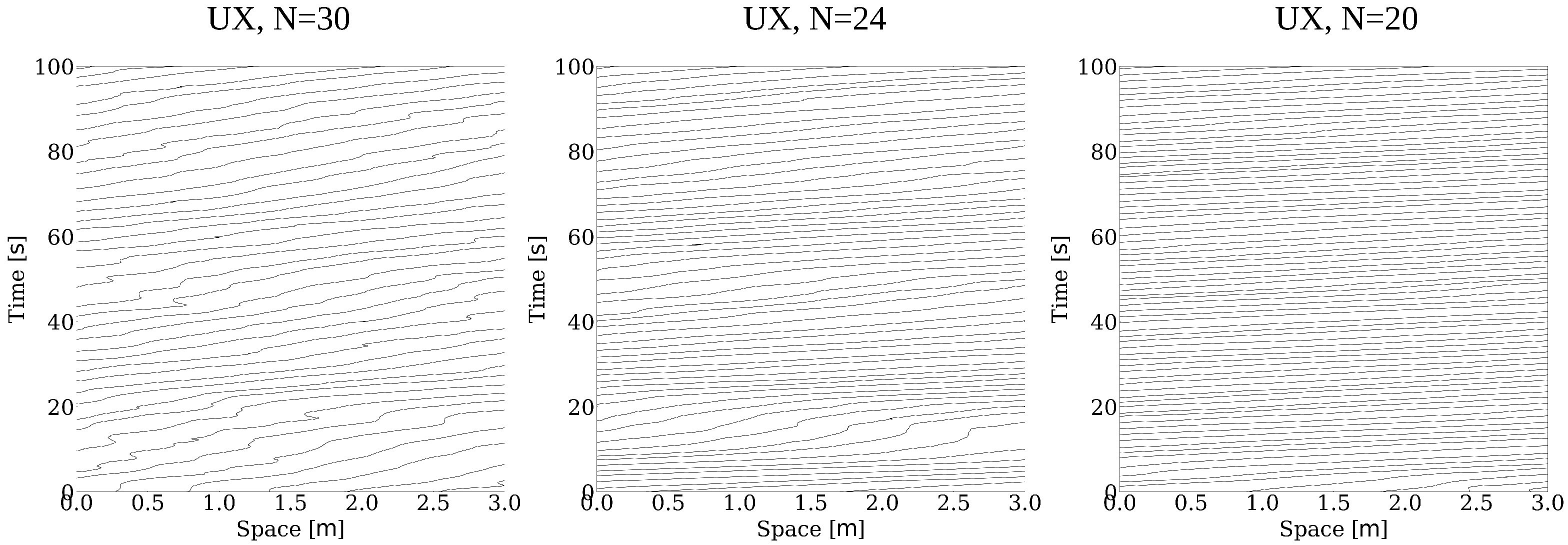In the Palestine experiments, the data were obtained after performing several runs for pedestrians walking with the same gender composition (homogeneous: females alone and males alone) or mixed (heterogeneous: males and females walking together) (see Figure 1). Our analysis will utilize the mixed-gender (UX, N = 20, 24, 30), female (UF, N = 20), and male (UM, N = 20) experiments where N is the number of pedestrians in each run. In Figure 2, we see the trajectories of pedestrians in UX experiments over time. We notice the emergence of stop-and-go waves for high densities (N = 30), which means that the pedestrians start to adjust their positions to avoid collision.

The same measurement method as [26] is used to calculate the individual speed and headway for pedestrians walking at each time frame. The speed of the pedestrian i is calculated at time t as follows:

$$v_i\left(t\right)=\frac{x_i(t+\Delta t/2)-x_i(t-\Delta t/2)}{\Delta t},$$

(4)

where $\Delta t$ is a short time constant (10 frames, 0.4 s) and $x_i\left(t\right)$ is the x coordinate of pedestrian’s i position at time t. We use the small value of $\Delta t=0.4$ s to smooth the trajectories in order to avoid fluctuation of the pedestrian’s step [27].

The headway is defined as the distance between a pedestrian i and its predecessor $i+1$:

$$h_i\left(t\right)=x_{i+1}\left(t\right)-x_i\left(t\right),$$

(5)

where $x_{i+1}$ and $x_i$ are the x coordinates of predecessor and subject pedestrian at time t, respectively.

These calculated movement quantities and associated pedestrian information are utilized as inputs to the FFNN.

Table 1. This table shows the descriptive statistics (number of pedestrians (N), mean, and standard deviation) for the Palestine dataset [26]. The second column contains the inputs and output that are used for the proposed FFNNs.

Experiment	Factor	No. of Samples	Mean	SD	N
UX	Subject PD * speed (m/s)	15,893	0.219	0.111	15, 20, 24, 30
	Subject PD headway (m)		0.595	0.11
	Predecessor PD headway (m)		0.608	0.124
	Follower PD headway (m)		0.588	0.109
UF	Subject PD speed (m/s)	422	0.615	0.102	20
	Subject PD headway (m)		0.711	0.104
	Predecessor PD headway (m)		0.731	0.111
	Follower PD headway (m)		0.712	0.120
UM	Subject PD speed (m/s)	443	0.660	0.095	20
	Subject PD headway (m)		0.694	0.136
	Predecessor PD headway (m)		0.689	0.121
	Follower PD headway (m)		0.706	0.143
UX	Subject PD speed (m/s)	435	0.500	0.104	20
	Subject PD headway (m)		0.717	0.119
	Predecessor PD headway (m)		0.693	0.128
	Follower PD headway (m)		0.704	0.126

^* PD is the abbreviation for “pedestrian”.

shows the descriptive statistics of the input and the output data we fed into the FFNNs. The first column presents the inputs (subject, predecessor, and follower pedestrian’s headway distances) and the output (subject pedestrian speed).

4. Structure of the Networks and Input Features

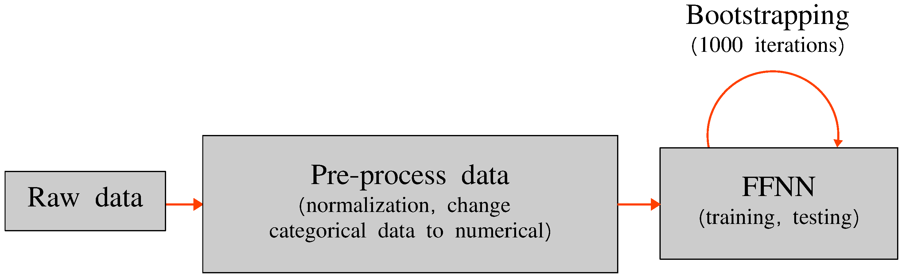
We apply several FFNNs to investigate the influence of interaction range (the distances with the neighbors) on pedestrian speed. These networks are fed with various input features for training. We analyze the results using cross-validation to control eventual prediction overfitting and to determine the optimal complexity of the networks in terms of layer and neuron numbers [28]. In this technique, we resample the dataset by randomly dividing the total dataset to 80% for training (i.e., UX experiments: 12,715 observations) and 20% for testing (i.e., UX experiments: 3178 observations). Furthermore, multiple iterations are applied following the bootstrap resampling technique to evaluate the error estimate precision and be able to determine whether an error difference is statistically significant [29,30] (see Figure 3). Randomly subsampling the training and testing datasets allows us to obtain a distribution of the errors instead of a point estimate. The estimation is finally performed using the average of bootstrap subsamples error, whereas the precision of estimation is evaluated using the bootstrap confidence interval represented as a boxplot. To quantify the error between the predicted and real values of the speed, we use the mean squared error (MSE) loss function:

$$\mathrm{MSE}=\frac{1}{n}\sum _{i=1}^n{(Y_i-\widehat{Y_i})}^2,$$

(6)

where n is the number of observations, Y is the vector of real speed values, and $\widehat{Y}$ is the vector of predicted values.

The developed networks are trained using the Adam optimizer [31], with a learning rate of $lr=0.003$. During the training phase, the hyperparameters, namely the number of hidden layers and the number of hidden neurons, are tuned to reach a robust model. In addition, the back-propagation algorithm [32] is used for training FFNNs by updating the weights’ values. We fit the model using different epoch sizes and a batch size of 10, which in most cases is sufficient to verify the progress of learning. Moreover, the Sigmoid activation function is applied for all layers in the different versions of the developed algorithm. Finally, to build a prototype for the proposed prediction model, the Keras framework [33] is utilized.

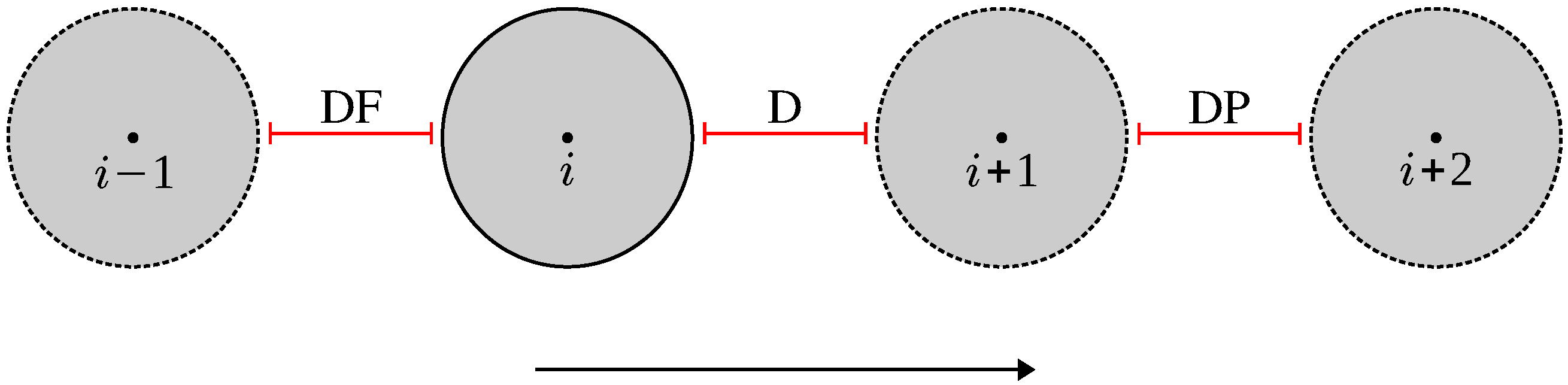
Different versions of the proposed FFNN are employed, varying in the number of input features fed into the input layer. These inputs indicate the movement characteristics of pedestrians walking in a single-file experimental setup. In the analysis, we focus on different combinations of the following headway distances as inputs:

• Subject pedestrian headway (D);
• Predecessor pedestrian headway (DP);
• Follower pedestrian headway (DF).

Figure 4 illustrates the 1D path of single-file movement experiments, considering four pedestrians in the video frame. In the UX experiments, the people are distributed in an ordered manner (pedestrian i gender is male, female, male, etc.).

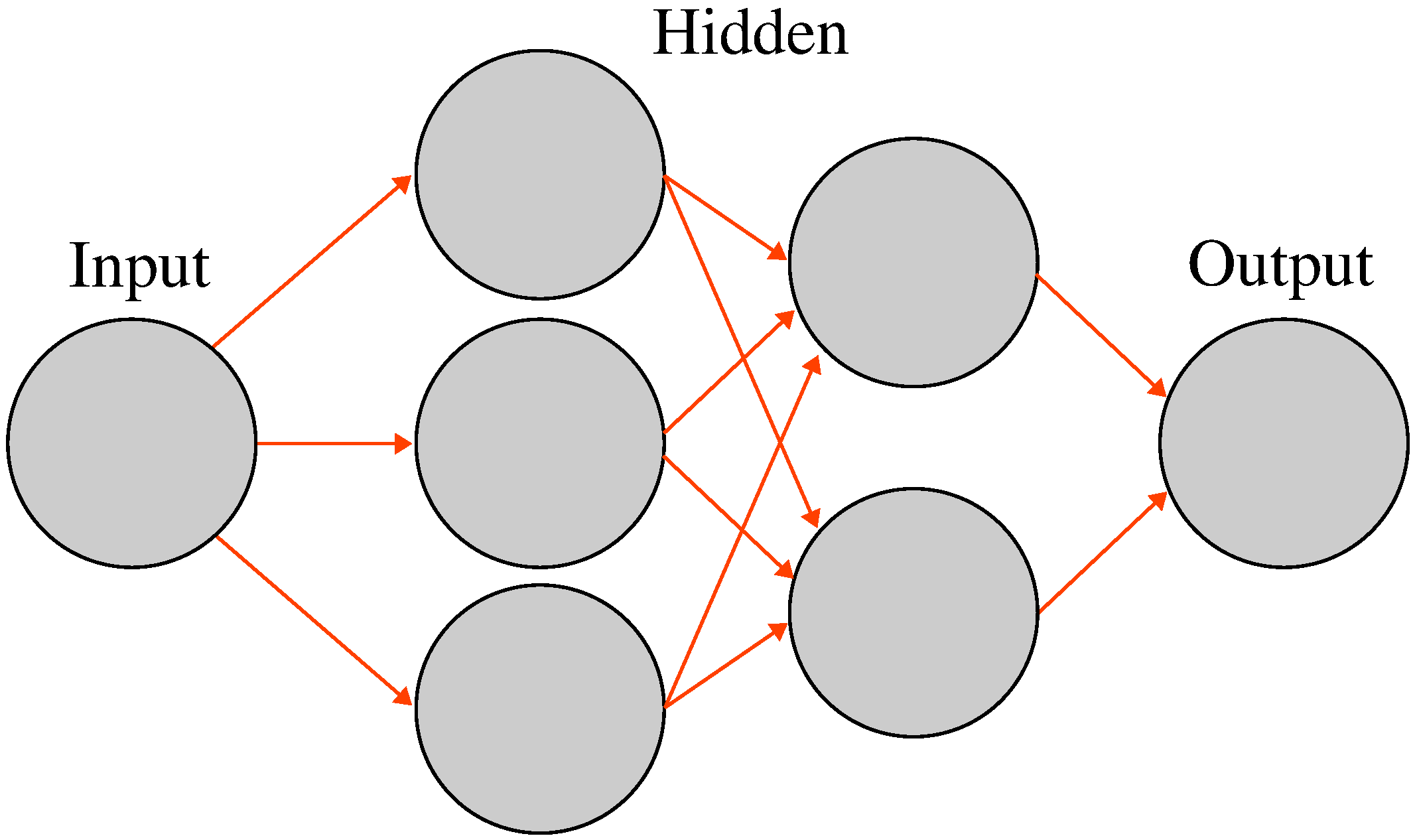
There is no standard approach for determining how many hidden layers and neurons should be used when building a prediction algorithm. Therefore, we follow Heaton’s [34] approach, where it is recommended to set the number of the hidden layers to be between the number of input features and the number of outputs. We test several combinations of hidden layers and neurons, ranging from neural networks with one hidden layer and one hidden neuron (i.e., shallow neural networks or logistics approach) to more complex networks with multiple layers and neurons (deep neural network). This makes the analysis global, starting from a basic statistical approach (a logistic regression) to complex networks, and allows for the comparison of different modeling approaches. We tried several combinations of hidden layers and neurons (1), (2), (3), (3, 2), (2, 2), (32, 32), and (64), where (x) represents one hidden layer with x number of hidden neurons. The expression (x, y) represents two hidden layers, with a number x of hidden neurons in the first layer and a number y of neurons in the second hidden layer. The prediction results show that the FFNN structure with two hidden layers (3, 2) (the first and second layers with three and two perceptrons, respectively) (see Figure 5) is enough for speed prediction with our dataset.

5. Results and Analysis

Our research aims to investigate the influence of the follower, predecessor, and second predecessor pedestrians’ headway distances on the speed behavior of a pedestrian. The investigation examines the isotropic nature of the interaction behavior, considering that a pedestrian interacts not only with pedestrians in their field of vision to regulate the speed but also with the pedestrians behind. We start training and testing several FFNNs with the Palestine dataset. To estimate the importance of different input features $(DF,D,DP)$ on predicting the speed of pedestrians, we first feed each distance alone to the FFNN and then a combination of features. Seven networks with different input features are developed and validated:

• In the networks $DF$, D, $DP$, we have one input feature for each network: the headway distance of the follower pedestrian, subject pedestrian, and the predecessor pedestrian, respectively.
• In networks $(DF+D)$, $(DF+DP)$, and $(D+DP)$, we predict the speed as a function of combinations of distances in front and behind to investigate the anisotropy of the pedestrians’ interaction behavior.
• The $\left(all\right)$ network fed with the headway distances of the subject pedestrian and neighbors altogether $(DF+D+DP)$.

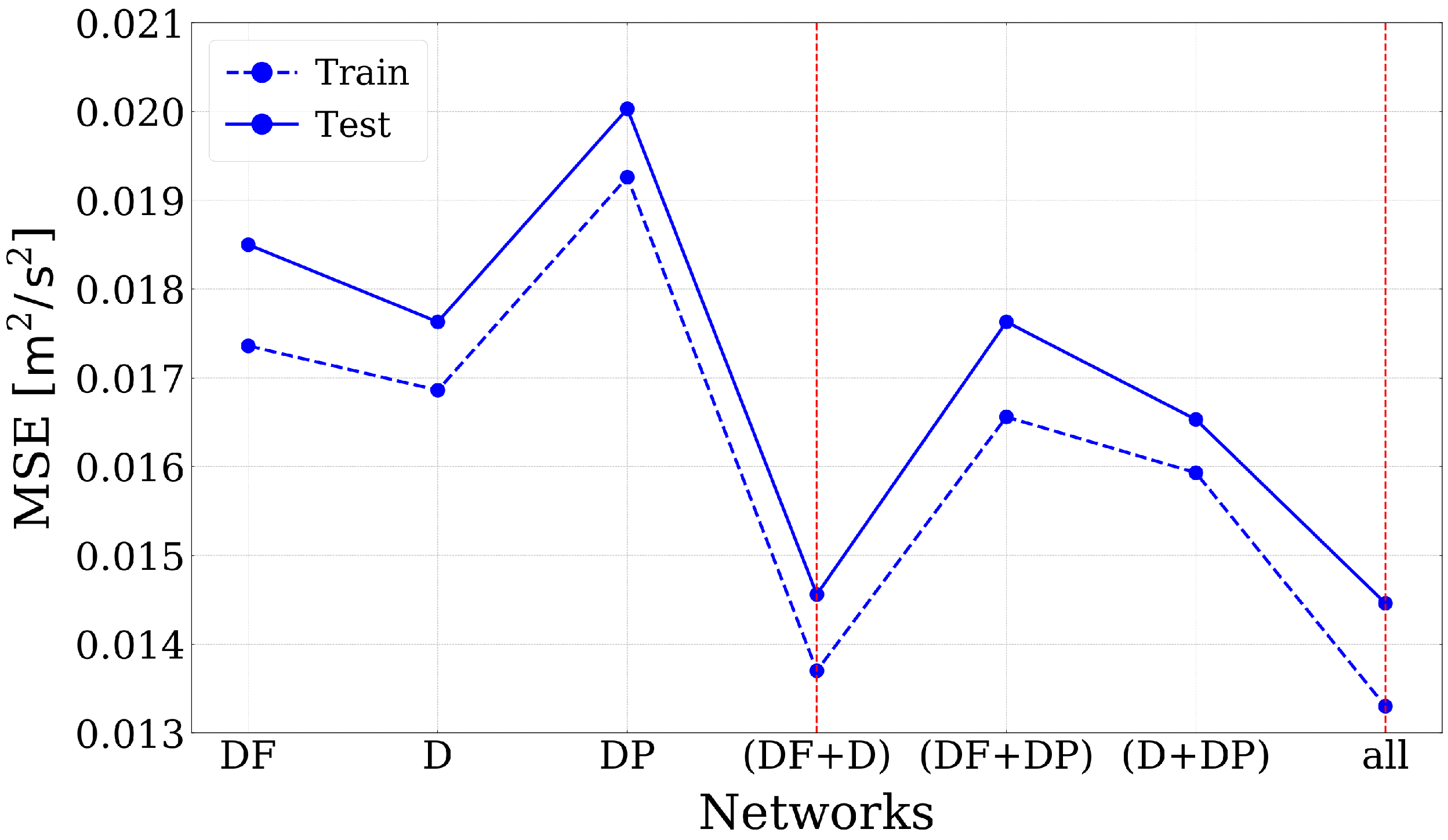
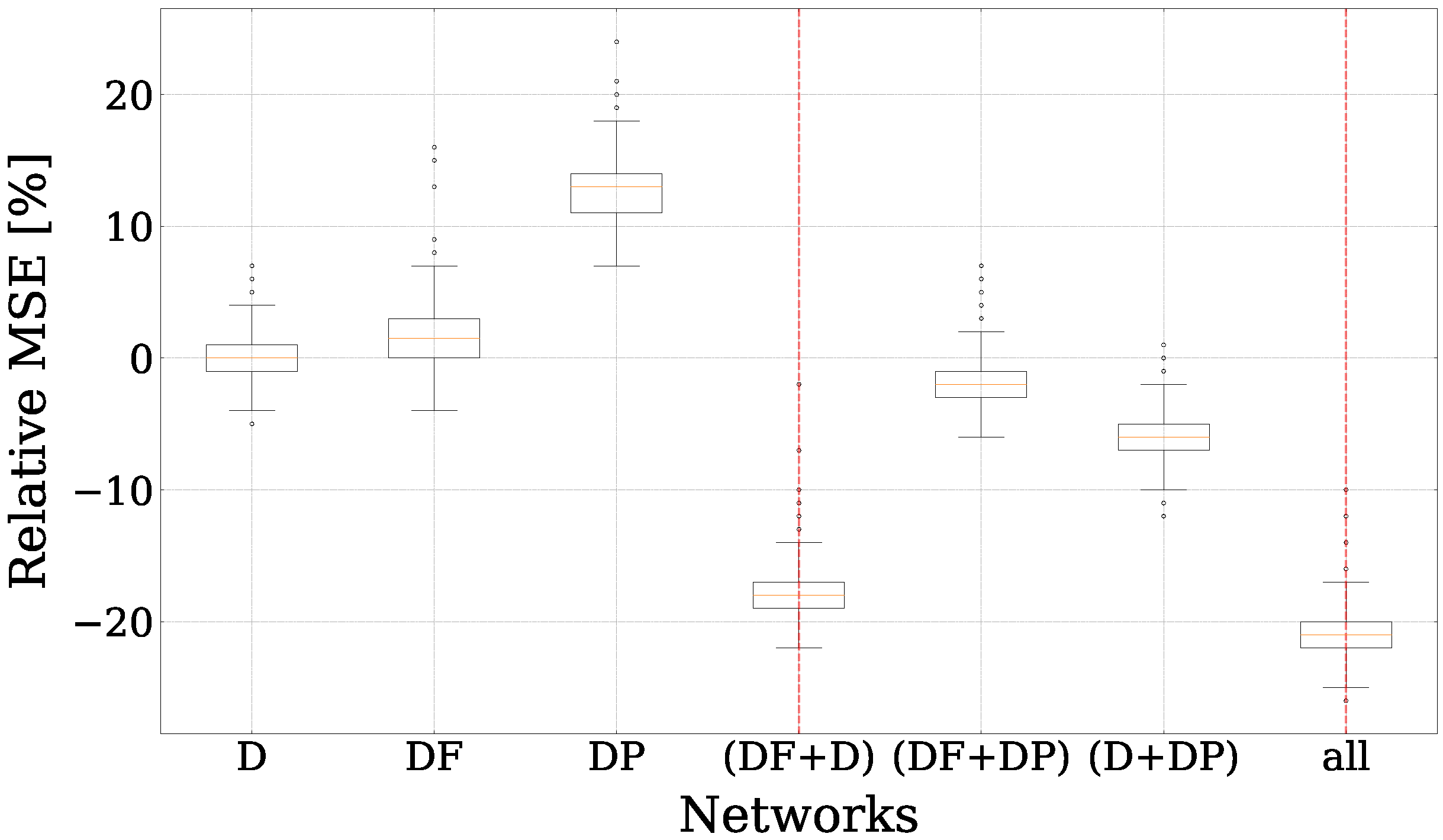
In Figure 6, the MSE values of the algorithms are visualized for training and testing phases using UX experiments, N = 20, 24, 30 samples. As we can see, the gap between the training and testing MSE results is not wide. That means the algorithms are reliable, and there are no overfitting problems. It is also observed that the speed prediction is enhanced with increasing input features. Figure 7 shows the relative MSEs of the algorithms taking D-input network for comparison. We predict the individual speed by training the networks for several iterations following the bootstrap approach. Considering the impact of the influential factors, we compare the networks with the same number of inputs together. In networks with one input feature, the D improves the estimation of speed by 1.5% compared to the $DF$ algorithm. That means the distance with a pedestrian in front has a greater impact on the speed prediction than the distance with the follower pedestrian. This result was confirmed previously, as the headway distance is the main dependency in many models [35]. Moreover, the algorithm with $DP$ increased the MSE by 13% compared to the D algorithm. This result indicates that the headway distance of the second predecessor has no significant influence on the subject pedestrian’s speed. In the case of two input factors, the algorithm $(DF+D)$ improves the performance of speed prediction by 16% and 11% in comparison with the $(DF+DP)$ and $(D+DP)$ networks, respectively. Interestingly, the combination of distance with the pedestrian in front and right behind improves the speed prediction compared to the combination of headway distances in front. From observing experiment videos, we notice that the pedestrians in relatively high densities start to adjust their speed when they approach the nearest neighbors to avoid colliding. This result demonstrates that the interaction behavior is not strictly anisotropic in single-file movement, contrary to classical modeling approaches that assume that only the front distances influence the speed. Therefore, it is suggested that a dynamical model that considers both distances D and $DF$ is likely to describe more aspects of the single-file dynamics. Finally, the $\left(all\right)$ algorithm that was fed with all headway distances as inputs improves the results by 21% compared to the D algorithm (3% compared to the $(DF+D)$ algorithm). This result indicates that with many input features, we can improve the speed estimation with percent corresponding to the impact of the inputs.

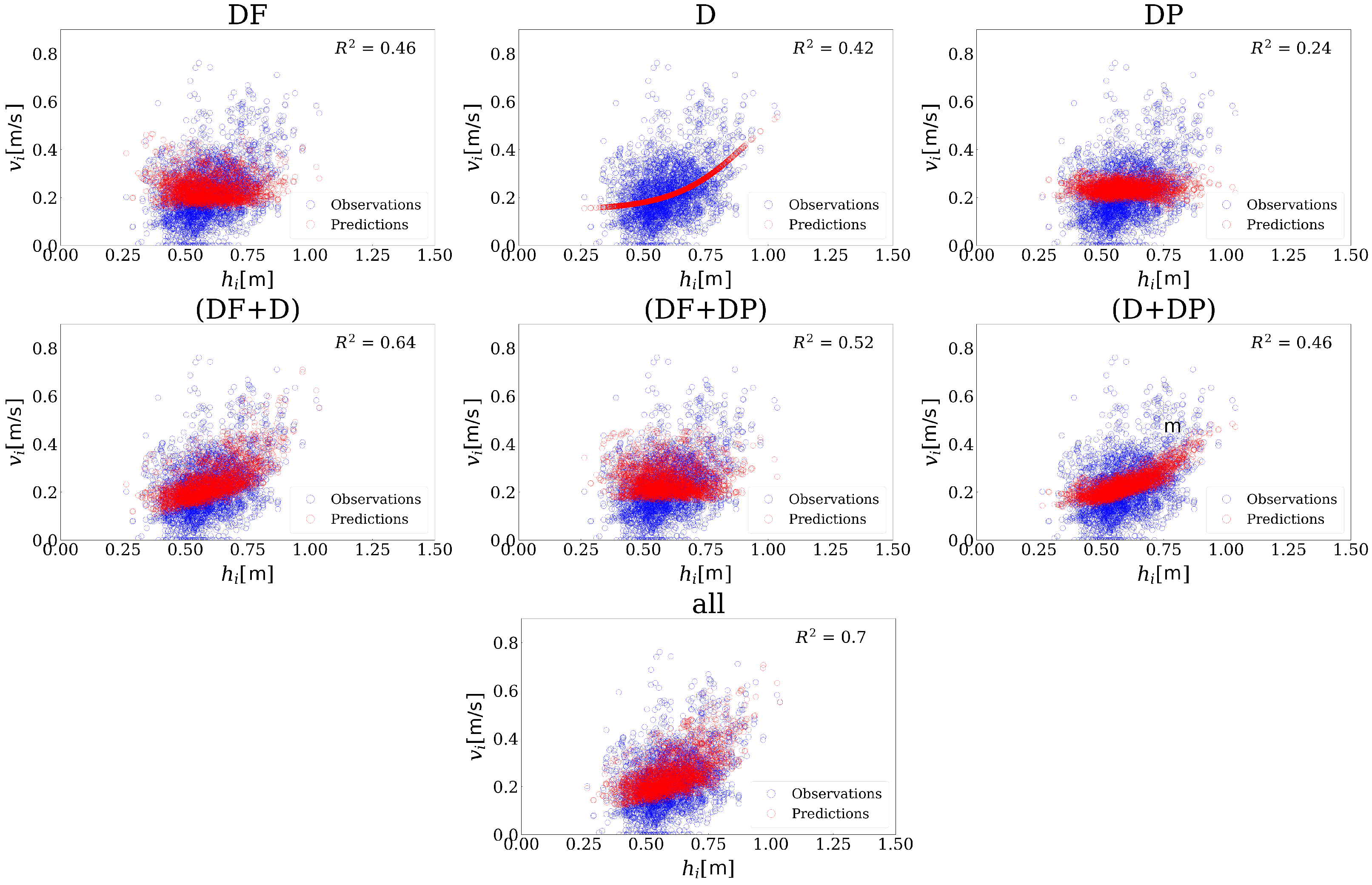
Figure 8 visualizes the relationship between the subject pedestrian headway distances and the speed values (actual and predicted) for different networks fed with UX, N = 20, 24, 30 data samples. The networks with the higher number of inputs can recapture the variability of the data points. As shown in the sub-figures, the algorithms with the optimal speed prediction results (best input combinations) have the highest $R^2$ values ($(DF+D)$ and $\left(all\right)$). In other words, the optimal algorithms capture the data points’ variability better than algorithms with inputs of low impact on the speed.

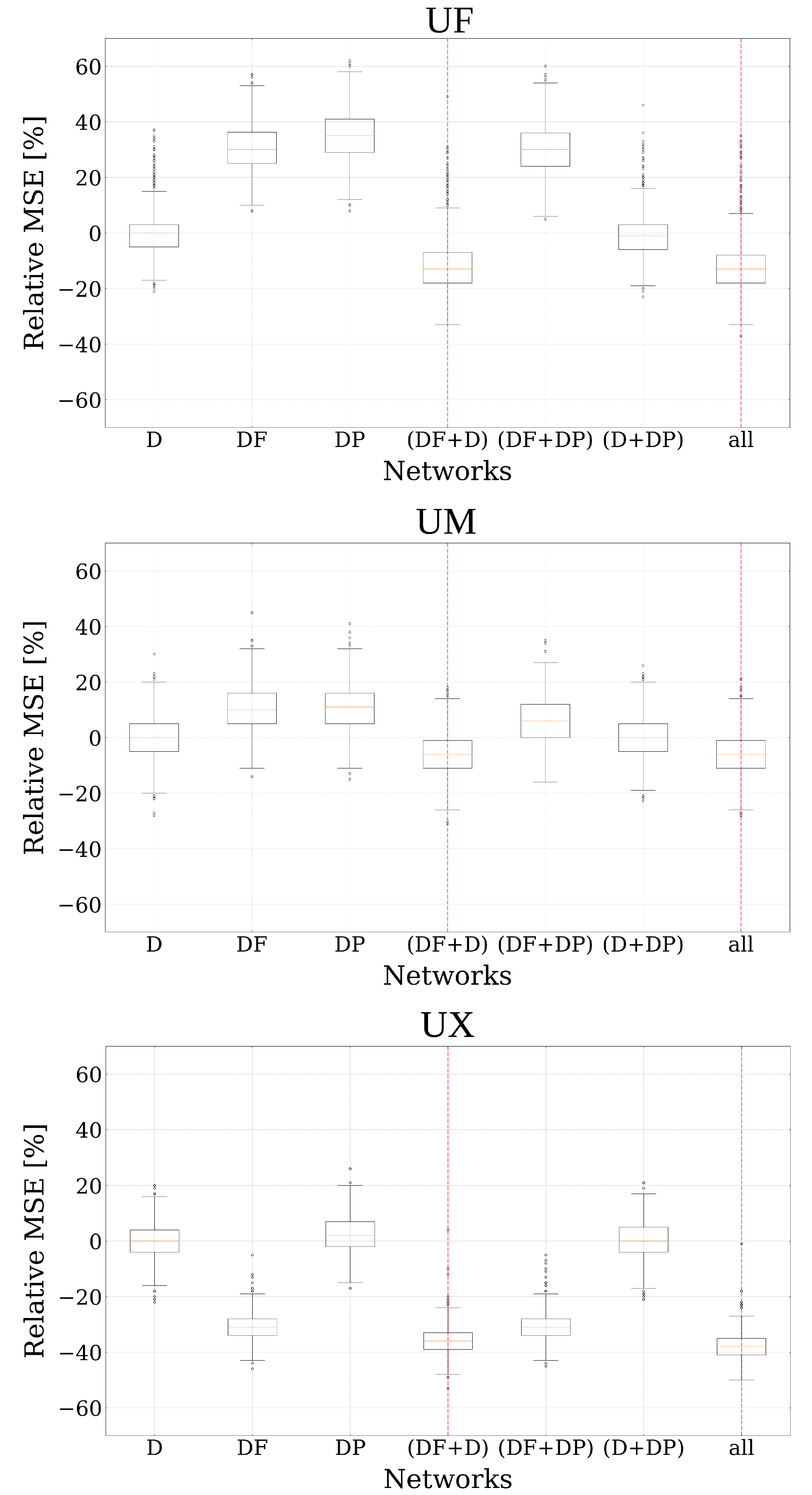
To investigate the influence of the different distances in front and behind in heterogeneous and homogenous gender groups, we trained the same FFNN structure with data for experiments UF, UM, and UX with N = 20 pedestrians. As shown in Figure 9, the distance to the pedestrian behind significantly improves the speed prediction compared to the distance in front for experiments UF, UM, and UX as well. For the UX experiments (N = 20), the improvement provided by the distance behind is significant, 36%, compared to the D algorithm (see Figure 9, UX). It is less for experiments UF and UM composed of solely female (14%) and males (7%). Furthermore, the small sizes of the samples do to not allow us to systematically demonstrate statistically that the differences are significant, as the boxplots partly overlap. Nevertheless, the influence of the distance behind is observed for flow solely composed of males and females, especially for the females. It is, however, clearly more pronounced for the mixed gender flow. Therefore, it does not exclude that gender effects in the mixed flow, alternating male and female, reinforce the influence of the pedestrian behind. Further empirical analysis with more data samples should emphasize the influence of distance behind on pedestrian speed for homogeneous or random mixed gender groups.

6. Conclusions

This article investigates the impact of headway distances and the interaction range on pedestrian movement by means of FFNN. Previous research generally assumes that pedestrian movement is mostly influenced by people in their field of vision, i.e., in the direction of motion. Such question rely on the anisotropic nature of pedestrian interaction behavior. In our research, we analyze the influence of the range of interaction with the distances behind and in front on pedestrian speed in single-file movement experiments. We predict the speed of pedestrians using a single-file experimental dataset performed in Palestine including uniformly mixed and homogeneous gender flow. Because relatively simple mechanisms primarily govern single-file movement, our investigation reveals that a shallow feedforward neural network structure (3, 2) is sufficient to optimally fit the data.

We explore several algorithms by changing the number and type of input distance features. The findings show that a prediction algorithm including the distance to the follower pedestrian as an input feature improves the MSE results by a factor up to 18% compared to an algorithm solely based on the distance in front. Such improvement may reach up to 36% for certain experiments. Taking into account the headway distance of the second predecessor has no strong influence on subject pedestrian’s speed. Even if they are still significantly observed for gender homogeneous flow, such features are especially pronounced for uniform mixed gender experiments. Therefore, we do not exclude that the influence on the motion of the pedestrian behind is reinforced by gender effects.

Much previous research assumes that the pedestrian motion is strongly anisotropic, i.e., mostly influenced by the environment in the direction of motion. However, we observe that the distance behind in single-file motion plays a role in the dynamic. These results suggest that the follower headway ($DF$) is a potential influential factor that significantly improves the prediction of pedestrian speed. It might be considered a modeling input. Yet the correlation we observe may be the consequence of an anisotropic mechanism. Such an assumption should be tested using isotropic and anisotropic models.

For homogeneous gender groups (UF and UM), we notice that the distance behind the pedestrian influences the prediction of the speed. This is especially the case for the experiments with females. However, further empirical analysis with more data samples is needed to highlight this conclusion. For future work, we aim to experiment and generalize the anisotropy of pedestrian behavior for more complex geometries and dynamics and to take into account further factors in addition to gender, e.g., cultural and age effects.