
Artificial Jellyfish Optimization with Deep-Learning-Driven Decision Support System for Energy Management in Smart Cities

 , ,
, ,
Abstract
:1. Introduction
2. Related Works
3. The Proposed Model
3.1. Design of CNN-ABLSTM-Based Predictive Model
3.2. Hyperparameter Optimization
| Algorithm 1: Pseudocode of AJO algorithm |
| Begin Determine the objective function Fix the searching space, population size and maximal iteration Initialize the population of JF, , utilizing a logistic chaotic map Compute the quantity of food at all Define the JF at place presently with most food Initializing time: Repeat For nPop do Compute the time control utilization If : the JF follows the ocean current (1) Define the ocean current (2) Novel place of JF was determined Else: the JF moves inside a swarm If rand(0,1) : the JF displays type A motion (passive motion) (1) Novel place of JF was determined Else: JF displays type motion (active motion) (2) Define the direction of JF (3) Novel place of JF was determined End if End if Verify the boundary condition and compute the quantity of food at novel place Upgrade the place of JF and place of JF presently with the food End for Upgrade the time: Still end condition was met Output the optimal outcomes and visualize (JF bloom) End |
4. Results and Analysis
4.1. Dataset Details
4.2. Result Analysis
5. Discussion
6. Conclusions
Author Contributions
Funding
Institutional Review Board Statement
Informed Consent Statement
Data Availability Statement
Conflicts of Interest
References
- Calvillo, C.F.; Sánchez-Miralles, A.; Villar, J. Energy management and planning in smart cities. Renew. Sustain. Energy Rev. 2016, 55, 273–287. [Google Scholar] [CrossRef] [Green Version]
- Liu, Y.; Yang, C.; Jiang, L.; Xie, S.; Zhang, Y. Intelligent edge computing for IoT-based energy management in smart cities. IEEE Network 2019, 33, 111–117. [Google Scholar] [CrossRef]
- Mahapatra, C.; Moharana, A.K.; Leung, V. Energy management in smart cities based on internet of things: Peak demand reduction and energy savings. Sensors 2017, 17, 2812. [Google Scholar] [CrossRef] [Green Version]
- Sirohi, P.; Al-Wesabi, F.N.; Alshahrani, H.M.; Maheshwari, P.; Agarwal, A.; Dewangan, B.K.; Hilal, A.M.; Choudhury, T. Energy-efficient cloud service selection and recommendation based on qos for sustainable smart cities. Appl. Sci. 2021, 11, 9394. [Google Scholar] [CrossRef]
- Alsubaei, F.S.; Al-Wesabi, F.N.; Hilal, A.M. Deep learning-based small object detection and classification model for garbage waste management in smart cities and iot environment. Appl. Sci. 2022, 12, 2281. [Google Scholar] [CrossRef]
- Al-Qarafi, A.; Alrowais, F.; Alotaibi, S.; Nemri, N.; Al-Wesabi, F.N.; Duhayyim, A.; Marzouk, R.; Othman, M.; Al-Shabi, M. Optimal machine learning based privacy preserving blockchain assisted internet of things with smart cities environment. Appl. Sci. 2022, 12, 5893. [Google Scholar]
- Kamienski, C.A.; Borelli, F.F.; Biondi, G.O.; Pinheiro, I.; Zyrianoff, I.D.; Jentsch, M. Context design and tracking for IoT-based energy management in smart cities. IEEE Internet Things J. 2017, 5, 687–695. [Google Scholar] [CrossRef]
- Petrović, N.; Roblek, V.; Nejković, V. Mobile Applications and Services for Next-Generation Energy Management in Smart Cities. Sustain. Dev. 2020, 1, 2. [Google Scholar]
- Laroui, M.; Dridi, A.; Afifi, H.; Moungla, H.; Marot, M.; Cherif, M.A. Energy management for electric vehicles in smart cities: A deep learning approach. In Proceedings of the 2019 15th International Wireless Communications & Mobile Computing Conference (IWCMC), IEEE, Tangier, Morocco, 24–28 June 2019; pp. 2080–2085. [Google Scholar]
- Shreenidhi, H.S.; Ramaiah, N.S. A two-stage deep convolutional model for demand response energy management system in IoT-enabled smart grid. Sustain. Energy Grids Netw. 2022, 30, 100630. [Google Scholar]
- Lotfi, M.; Almeida, T.; Javadi, M.S.; Osório, G.J.; Monteiro, C.; Catalão, J.P. Coordinating energy management systems in smart cities with electric vehicles. Appl. Energy 2022, 307, 118241. [Google Scholar] [CrossRef]
- Elsisi, M.; Tran, M.Q.; Mahmoud, K.; Lehtonen, M.; Darwish, M.M. Deep learning-based industry 4.0 and Internet of Things towards effective energy management for smart buildings. Sensors 2021, 21, 1038. [Google Scholar] [CrossRef] [PubMed]
- Vázquez-Canteli, J.R.; Ulyanin, S.; Kämpf, J.; Nagy, Z. Fusing TensorFlow with building energy simulation for intelligent energy management in smart cities. Sustain. Cities Soc. 2019, 45, 243–257. [Google Scholar] [CrossRef]
- Xiaoyi, Z.; Dongling, W.; Yuming, Z.; Manokaran, K.B.; Antony, A.B. IoT driven framework based efficient green energy management in smart cities using multi-objective distributed dispatching algorithm. Environ. Impact Assess. Rev. 2021, 88, 106567. [Google Scholar] [CrossRef]
- Ullah, I.; Hussain, I.; Uthansakul, P.; Riaz, M.; Khan, M.N.; Lloret, J. Exploiting multi-verse optimization and sine-cosine algorithms for energy management in smart cities. Appl. Sci. 2020, 10, 2095. [Google Scholar] [CrossRef] [Green Version]
- Kim, D.; Kwon, D.; Park, L.; Kim, J.; Cho, S. Multiscale LSTM-based deep learning for very-short-term photovoltaic power generation forecasting in smart city energy management. IEEE Syst. J. 2020, 15, 346–354. [Google Scholar] [CrossRef]
- Hrnjica, B.; Mehr, A.D. Energy demand forecasting using deep learning. In Smart Cities Performability, Cognition, & Security; Springer: Cham, Switzerland, 2020; pp. 71–104. [Google Scholar]
- Li, X.; Liu, H.; Wang, W.; Zheng, Y.; Lv, H.; Lv, Z. Big data analysis of the internet of things in the digital twins of smart city based on deep learning. Future Gener. Comput. Syst. 2022, 128, 167–177. [Google Scholar] [CrossRef]
- Siami-Namini, S.; Tavakoli, N.; Namin, A.S. The performance of LSTM and BiLSTM in forecasting time series. In Proceedings of the 2019 IEEE International Conference on Big Data (Big Data) IEEE, Los Angeles, CA, USA, 9–12 December 2019; pp. 3285–3292. [Google Scholar]
- Shan, L.; Liu, Y.; Tang, M.; Yang, M.; Bai, X. CNN-BiLSTM hybrid neural networks with attention mechanism for well log prediction. J. Pet. Sci. Eng. 2021, 205, 108838. [Google Scholar] [CrossRef]
- Chou, J.S.; Truong, D.N. A novel metaheuristic optimizer inspired by behavior of jellyfish in ocean. Appl. Math. Comput. 2021, 389, 125535. [Google Scholar] [CrossRef]
- Abdel-Basset, M.; Mohamed, R.; Chakrabortty, R.K.; Ryan, M.J.; El-Fergany, A. An improved artificial jellyfish search optimizer for parameter identification of photovoltaic models. Energies 2021, 14, 1867. [Google Scholar] [CrossRef]
- Individual Household Electric Power Consumption Data Set. Available online: https://archive.ics.uci.edu/ml/datasets/individual+household+electric+power+consumption (accessed on 12 March 2022).
- England, I.N. Available online: https://www.iso-ne.com/system-planning/system-forecasting/load-forecast/ (accessed on 12 March 2022).
- Han, T.; Muhammad, K.; Hussain, T.; Lloret, J.; Baik, S.W. Efficient Deep Learning Framework for Intelligent Energy Management in IoT Networks. IEEE Internet Things J. 2020, 8, 3170–3179. [Google Scholar] [CrossRef]
- Lv, P.; Liu, S.; Yu, W.; Zheng, S.; Lv, J. EGA-STLF: A Hybrid Short-Term Load Forecasting Model. IEEE Access 2020, 8, 31742–31752. [Google Scholar] [CrossRef]
- Tan, M.; Yuan, S.; Li, S.; Su, Y.; Li, H.; He, F. Ultra-short-term industrial power demand forecasting using LSTM based hybrid ensemble learning. IEEE Trans. Power Syst. 2019, 35, 2937–2948. [Google Scholar] [CrossRef]
- Chitalia, G.; Pipattanasomporn, M.; Garg, V.; Rahman, S.J.A.E. Robust short-term electrical load forecasting framework for commercial buildings using deep recurrent neural networks. Appl. Energy 2020, 278, 115410. [Google Scholar] [CrossRef]
- Sajjad, M.; Khan, Z.A.; Ullah, A.; Hussain, T.; Ullah2, W.; Lee, M.Y.; Baik, S.W. A novel CNN-GRU-based hybrid approach for short-term residential load forecasting. IEEE Access 2020, 8, 143759–143768. [Google Scholar] [CrossRef]
- Kim, T.-Y.; Cho, S.-B.J.E. Predicting residential energy consumption using CNN-LSTM neural networks. Energy 2019, 182, 72–81. [Google Scholar] [CrossRef]
- Abdel-Basset, M.; Hawash, H.; Chakrabortty, R.K.; Ryan, M. Energy-net: A deep learning approach for smart energy management in iot-based smart cities. IEEE Internet Things J. 2021, 8, 12422–12435. [Google Scholar] [CrossRef]


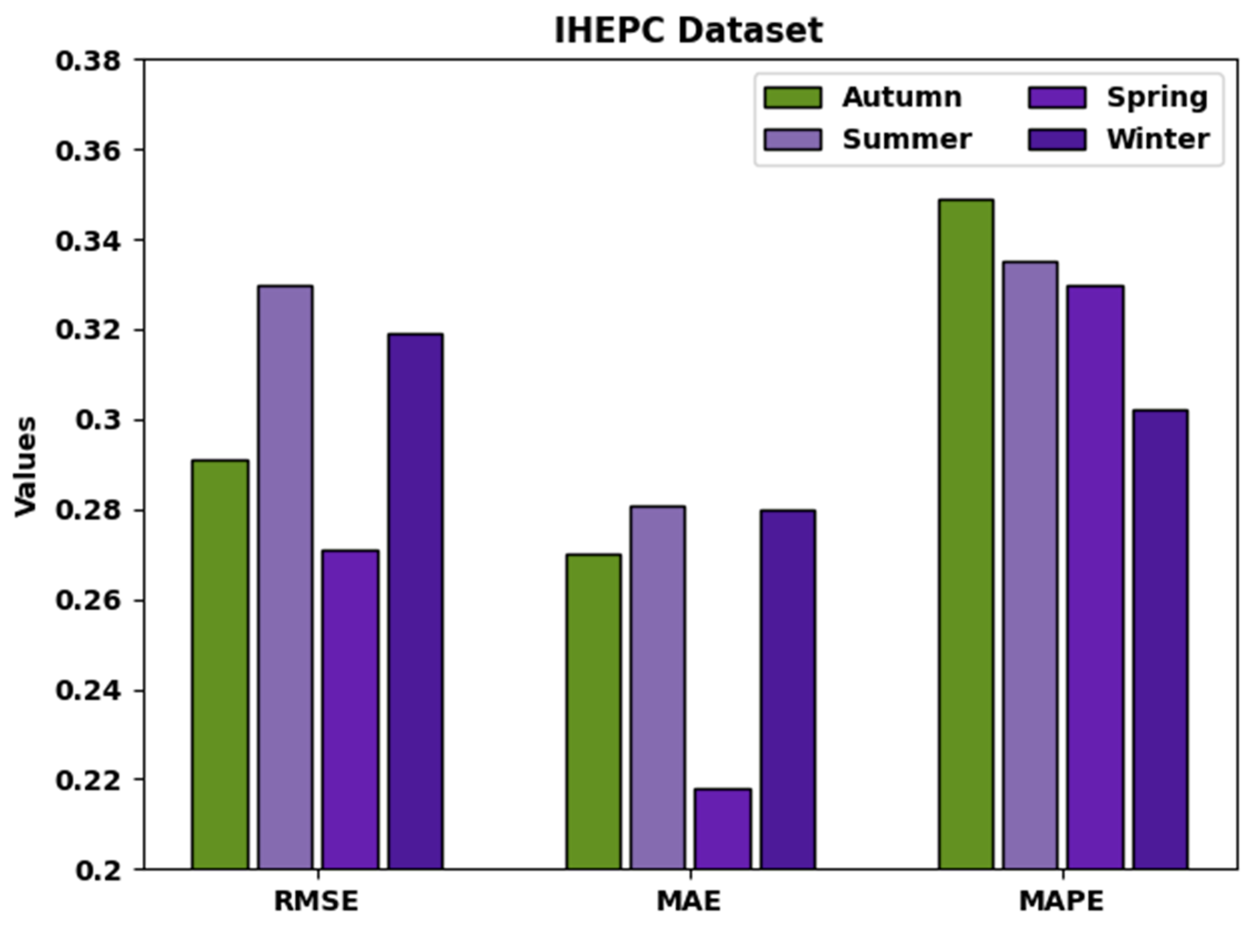
| Label | RMSE | MAE | MAPE |
|---|---|---|---|
| IHEPC Dataset | |||
| Autumn | 0.291 | 0.270 | 0.349 |
| Summer | 0.330 | 0.281 | 0.335 |
| Spring | 0.271 | 0.218 | 0.330 |
| Winter | 0.319 | 0.280 | 0.302 |
| Average | 0.303 | 0.262 | 0.329 |
| ISO-NE Dataset | |||
| Autumn | 0.413 | 0.333 | 0.256 |
| Summer | 0.453 | 0.364 | 0.241 |
| Spring | 0.480 | 0.422 | 0.218 |
| Winter | 0.479 | 0.416 | 0.231 |
| Average | 0.456 | 0.384 | 0.237 |
| Global Active Power—IHEPC Dataset | ||
|---|---|---|
| Time Steps (h) | Actual | Predicted |
| 0 | 1.053 | 0.890 |
| 20 | 4.308 | 4.383 |
| 40 | 0.334 | 0.223 |
| 60 | 0.422 | 0.580 |
| 80 | 1.532 | 1.387 |
| 100 | 0.321 | 0.302 |
| 120 | 0.283 | 0.187 |
| 140 | 1.368 | 1.309 |
| 160 | 0.182 | 0.222 |
| 180 | 1.961 | 1.762 |
| 200 | 0.478 | 0.415 |
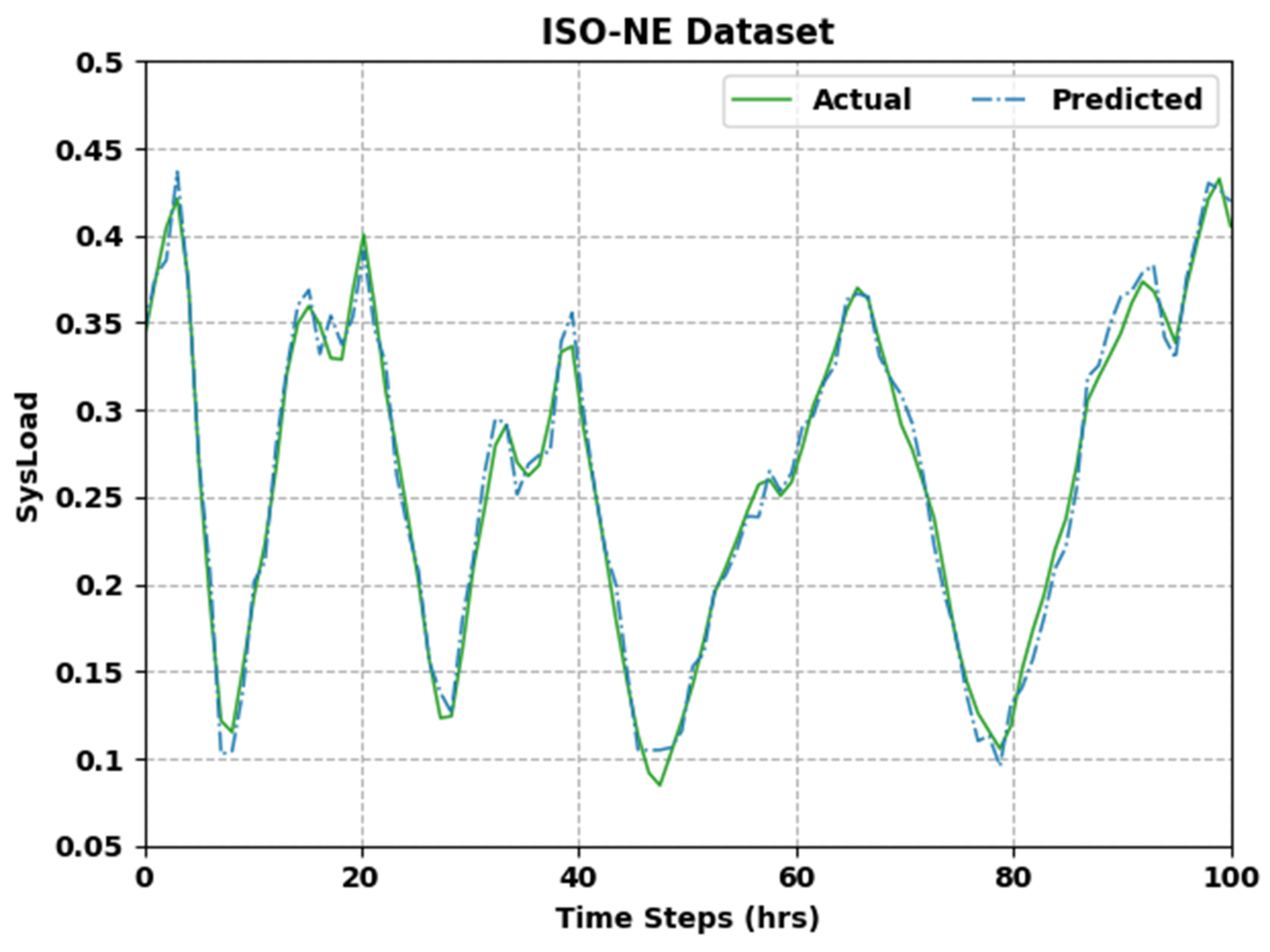
| System Load—ISO-NE Dataset | ||
|---|---|---|
| Time Steps (h) | Actual | Predicted |
| 0 | 0.341 | 0.345 |
| 10 | 0.190 | 0.199 |
| 20 | 0.401 | 0.394 |
| 30 | 0.198 | 0.201 |
| 40 | 0.309 | 0.322 |
| 50 | 0.131 | 0.133 |
| 60 | 0.266 | 0.278 |
| 70 | 0.285 | 0.302 |
| 80 | 0.125 | 0.139 |
| 90 | 0.345 | 0.365 |
| 100 | 0.406 | 0.420 |
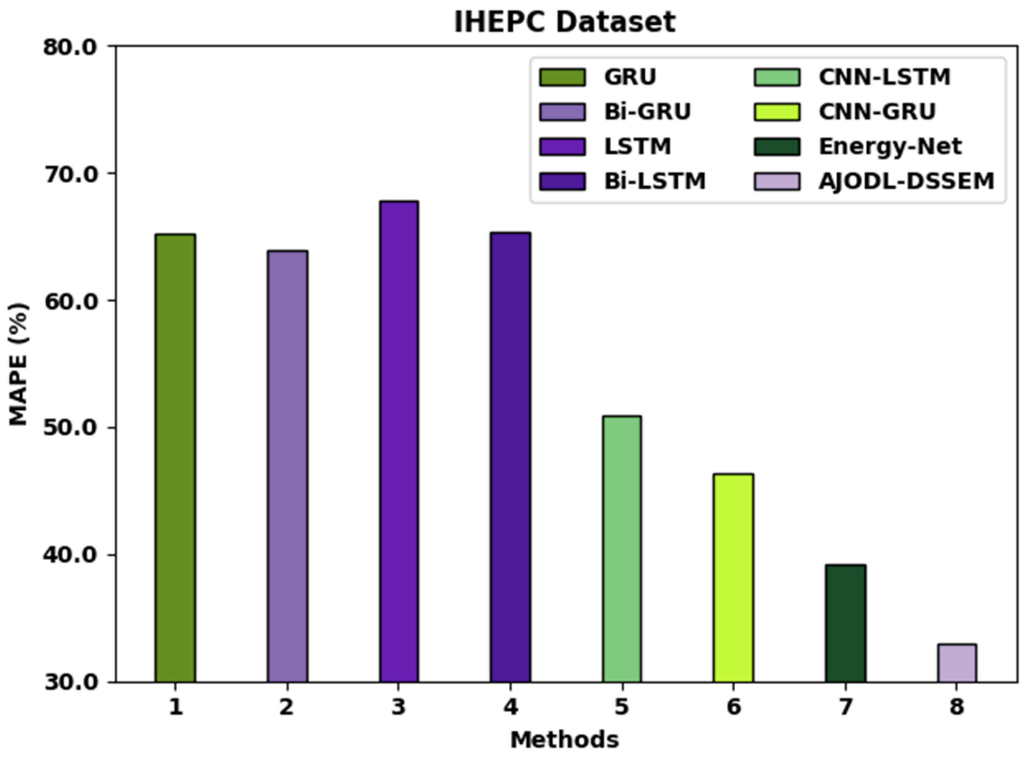
| IHEPC Dataset | ||||
|---|---|---|---|---|
| Models | MSE | RMSE | MAE | MAPE (%) |
| GRU [24] | 0.270 | 0.518 | 0.389 | 65.200 |
| Bi-GRU [25] | 0.251 | 0.501 | 0.372 | 63.900 |
| LSTM [26] | 0.413 | 0.643 | 0.409 | 67.800 |
| Bi-LSTM [27] | 0.422 | 0.647 | 0.392 | 65.300 |
| CNN-LSTM [28] | 0.431 | 0.662 | 0.403 | 50.900 |
| CNN-GRU [29] | 0.243 | 0.493 | 0.348 | 46.400 |
| Energy-Net [30] | 0.125 | 0.354 | 0.287 | 39.200 |
| AJODL-DSSEM | 0.092 | 0.303 | 0.262 | 32.900 |
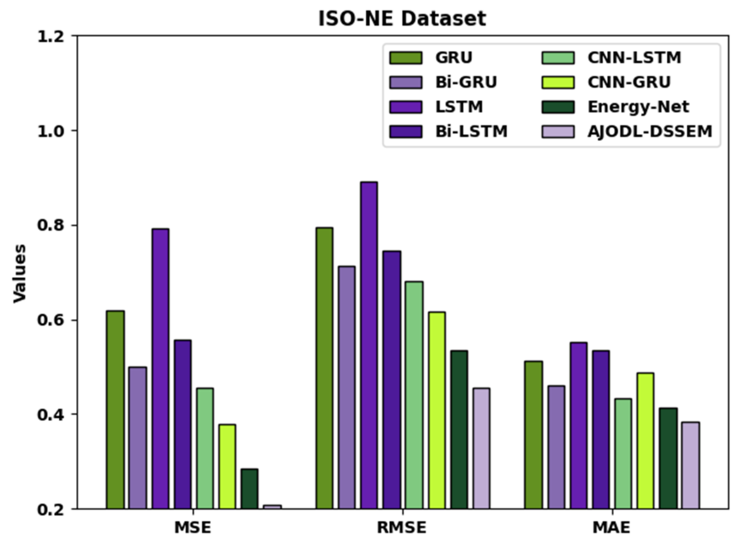
| ISO-NE Dataset | ||||
|---|---|---|---|---|
| Models | MSE | RMSE | MAE | MAPE (%) |
| GRU [24] | 0.619 | 0.794 | 0.513 | 49.200 |
| Bi-GRU [25] | 0.501 | 0.713 | 0.461 | 60.900 |
| LSTM [26] | 0.792 | 0.891 | 0.552 | 65.400 |
| Bi-LSTM [27] | 0.557 | 0.746 | 0.534 | 62.300 |
| CNN-LSTM [28] | 0.456 | 0.681 | 0.434 | 40.900 |
| CNN-GRU [29] | 0.379 | 0.617 | 0.488 | 34.100 |
| Energy-Net [30] | 0.286 | 0.535 | 0.414 | 29.300 |
| AJODL-DSSEM | 0.208 | 0.456 | 0.384 | 23.700 |
Publisher’s Note: MDPI stays neutral with regard to jurisdictional claims in published maps and institutional affiliations. |
© 2022 by the authors. Licensee MDPI, Basel, Switzerland. This article is an open access article distributed under the terms and conditions of the Creative Commons Attribution (CC BY) license (https://creativecommons.org/licenses/by/4.0/).
Share and Cite
Al-Qarafi, A.; Alsolai, H.; Alzahrani, J.S.; Negm, N.; Alharbi, L.A.; Al Duhayyim, M.; Mohsen, H.; Al-Shabi, M.; Al-Wesabi, F.N. Artificial Jellyfish Optimization with Deep-Learning-Driven Decision Support System for Energy Management in Smart Cities. Appl. Sci. 2022, 12, 7457. https://doi.org/10.3390/app12157457
Al-Qarafi A, Alsolai H, Alzahrani JS, Negm N, Alharbi LA, Al Duhayyim M, Mohsen H, Al-Shabi M, Al-Wesabi FN. Artificial Jellyfish Optimization with Deep-Learning-Driven Decision Support System for Energy Management in Smart Cities. Applied Sciences. 2022; 12(15):7457. https://doi.org/10.3390/app12157457
Chicago/Turabian StyleAl-Qarafi, A., Hadeel Alsolai, Jaber S. Alzahrani, Noha Negm, Lubna A. Alharbi, Mesfer Al Duhayyim, Heba Mohsen, M. Al-Shabi, and Fahd N. Al-Wesabi. 2022. "Artificial Jellyfish Optimization with Deep-Learning-Driven Decision Support System for Energy Management in Smart Cities" Applied Sciences 12, no. 15: 7457. https://doi.org/10.3390/app12157457