The Relation between Induced Electric Field and TMS-Evoked Potentials: A Deep TMS-EEG Study

Abstract

Transcranial magnetic stimulation (TMS) in humans induces electric fields (E-fields, EF) that perturb and modulate the brain’s endogenous neuronal activity and result in the generation of TMS-evoked potentials (TEPs). The exact relation of the characteristics of the induced E-field and the intensity of the brains’ response, as measured by electroencephalography (EEG), is presently unclear. In this pilot study, conducted on three healthy subjects and two patients with generalized epilepsy (total: 3 males, 2 females, mean age of 26 years; healthy: 2 males, 1 female, mean age of 25.7 years; patients: 1 male, 1 female, mean age of 26.5 years), we investigated the temporal and spatial relations of the E-field, induced by single-pulse stimuli, and the brain’s response to TMS. Brain stimulation was performed with a deep TMS device (BrainsWay Ltd., Jerusalem, Israel) and an H7 coil placed over the central area. The induced EF was computed on personalized anatomical models of the subjects through magneto quasi-static simulations. We identified specific time instances and brain regions that exhibit high positive or negative associations of the E-field with brain activity. In addition, we identified significant correlations of the brain’s response intensity with the strength of the induced E-field and finally prove that TEPs are better correlated with E-field characteristics than with the stimulator’s output. These observations provide further insight in the relation between E-field and the ensuing cortical activation, validate in a clinically relevant manner the results of E-field modeling and reinforce the view that personalized approaches should be adopted in the field of non-invasive brain stimulation.

1. Introduction

Transcranial magnetic stimulation (TMS) is a non-invasive brain stimulation technique based on the application of brief magnetic pulses that induce localized intracranial electrical fields (E-fields) and result in the excitation and/or inhibition of cortical neurons [1]. Thus, the magnetic stimuli modulate brain activity at the targeted area, causing transient alterations of cortical excitability and brain connectivity that have therapeutic implications in patients with neurological or psychiatric disorders [2,3,4]. In addition, TMS holds significant potential as a diagnostic and prognostic biomarker in numerous neurological disorders, such as epilepsy [5,6,7,8,9], stroke [10,11], multiple sclerosis [12,13] and Alzheimer’s disease [14,15]. Despite this progress, the precise neural mechanisms underlying the effects of TMS as well as the exact relation between the properties of the E-field and the brain’s physiological responses are incompletely understood and are a matter of active research [16].

Over the last couple of decades, the combination of electroencephalography with TMS (TMS-EEG) has emerged as a valuable clinical tool, but also as an innovative research approach for the investigation of brain circuits in health and disease [17,18]. In parallel, various attempts at the computational modeling of the E-field have taken place, ranging from relatively simple spherical models that approximate the head shape and rely on generic assumptions about the conductivity properties of intracranial tissues [19,20] to more advanced approaches, based on boundary or finite element methods (BEM and FEM, respectively) that take into full account the individual anatomy and scalp geometry [21,22]. The main aim of E-field modeling is to compare real with theoretical TMS responses [23], compare and test coil designs [24,25,26], predict the exact stimulation location and optimize stimulation parameters by guiding TMS coil positioning, orientation and dosimetry [19,27,28,29,30,31].

It is well known that in the case of TMS, the instantaneous E-field evokes action potentials in chains of excitatory and inhibitory cortical interneurons as well as principal output neurons in the cerebral cortex that are subsequently propagated intra- and inter-hemispherically, ultimately producing the recorded TMS-evoked potentials (TEPs). The overarching aim of the present work is to explore in detail the relation of the TMS-induced E-field and the brain’s physiological response. To this end, we posed two specific research questions.

The first one is as follows: What is the exact relation of the E-field induced at a certain stimulus intensity (SI), corresponding to a multiple (120% in our case) of the critical value of the lower cortical threshold (LT) to the ensuing global EEG response from a temporal (i.e., how does it change over time?) and spatial (i.e., where in the brain is it stronger?) point of view? The particular SI level was chosen on the basis of two criteria: (a) that it is clearly suprathreshold so as to secure the generation of TEPs, and (b) that it is sufficiently low so as to avoid the generation of biologic and non-biological artifacts, associated with high stimulus intensities, that may act as confounders.

The second question is: What is, in mathematical terms, the relation of the E-fields, induced by a wide range of peri-threshold stimulus intensities, with TEPs recorded in a particular brain region of interest (ROI)? The ROI was determined based on the results of the spatial correlation analysis (vide supra) and included nine centrally located electrodes.

In order to prove that the hypothesized relation between E-field and TEPs is present and significant not only under normal conditions, but also when cortical excitability has been demonstrably altered by disease and/or drug effects, we included not only healthy subjects but also patients with genetic generalized epilepsy receiving antiseizure medications.

In the next section of this manuscript, we briefly describe the protocol of the TMS-EEG study, the employed E-field computational model and data preprocessing and processing information. Then, in Section 3 and Section 4, we present and discuss the results of our analysis.

2. Materials and Methods

2.1. TMS Study Protocol and EEG Recording

For this TMS-EEG study, we employed an H7 coil (Brainsway Ltd., Jerusalem, Israel) [32] connected to a Magstim Rapid2 stimulator (Magstim, Spring Gardens, United Kingdom) and placed over the mid-line central area (i.e., 8 cm above the nasion along the main reference curve (nasion–inion) and conformal to the patient’s head). The H7 coil has a subdural depth and volume of stimulation of 3 cm and 40.3 cm³, respectively, without significantly increasing the E-fields induced at the superficial cortical structures [33] and is safe and effective for therapeutic applications [34,35,36]. During the TMS sessions, 1 electrooculographic (EOG) and 60 EEG signals were recorded continuously with Ag/AgCl pellet electrodes placed according to the international 10-10 system and connected to a TMS compatible EEG amplifier (eXimia, Nexstim Ltd., Helsinki, Finland). During acquisition, the reference channel was placed on the right mastoid and the ground electrode on the right zygomatic bone. The EEG signals were analog band-pass filtered from 0.1 to 500 Hz and sampled with a 1450 Hz sampling frequency and 16-bit precision. In order to reduce the TMS-induced artifact, the EEG amplifier was temporarily blocked from 100 µs before to 2 ms after the TMS pulse by a sample-and-hold circuitry [37]. Suppression of the TMS-related auditory evoked potentials was achieved with a psychophysically driven continuous white-based noise (WBN) mask combined with the use of earphones with highly effective insertion loss.

The study’s TMS-EEG protocol involved two stages. In the first stage, a wide range of SIs were used to determine visually the LT, i.e., the maximal SI that failed to produce a cortical response (TEP). This maximal SI was observed in more than one electrode in each subject, with most common electrode being C1. At this stage, we applied $n=30$ single stimuli per SI value, with an interstimulus interval (ISI) of 1000 ms. These records constitute Dataset A.

The LT was used as the basis for stage 2, where for each subject, a single record was produced at an SI of 120%LT with $n=100$ single stimuli and an ISI of 2000 ms. This set of records constitute Dataset B. Demographics of the participants (3 healthy subjects and 2 patients with genetic generalized epilepsy) and information regarding the TMS-EEG records are given in

Table 1. Subject demographics.

Subject ID	Age	Sex	Handedness	LT(%MSO)	Available SIs
S01 (H)	26	F	Right	32%	25–35%, 38% (120%LT)
S02 (H)	31	M	Right	30%	25–35%, 36% (120%LT)
S03 (H)	30	M	Right	30%	26–35%, 36% (120%LT)
S04 (P)	20	M	Right	28%	22–35%, 34% (120%LT)
S05 (P)	23	F	Right	27%	20–35%, 32% (120%LT)

. The first column provides the subject ID and condition (H for healthy and P for epileptic). Columns two to four have age, sex, and dominant hand information. The fifth column has the clinically determined LT as a percent of MSO. The final sixth column has the SIs tested for each subject in the determination of the subject-specific LT (Dataset A) and the SI for the 120% of LT (Dataset B).

2.2. E-Field Computation

The T1-weighted isotropic (1 mm × 1 mm × 1 mm voxel) magnetic resonance image (MRI) data of participants were used to generate their personalized anatomical head models in order to numerically calculate the induced EFs. The anatomical head models, consisting of white matter, grey matter, CSF and ventricles, bone and scalp, were initially automatically segmented by the headreco tool of the SimNIBS software package (SimNIBS Developers. SimNIBS 3.2.4) and then visually inspected, and manually customized when required, through the iSeg toolkit (ZMT Zurich MedTech & IT’IS foundation. iSeg).

Each head model, with its tissues assigned to standard electrical conductivities [38], was stimulated by the model of H7 coil. For the numerical computations of the electric field distribution inside the head, as induced by the TMS coil, we used the quasi-static low frequency solver of the computational life sciences software platform Sim4Life (ZMT ZurichMedTech, Zurich, Switzerland). This solver was used in the past for TMS calculations of various human anatomical models as implemented in another software platform, i.e., SEMCAD-X (SPEAG, Zurich, Switzerland) [39]. Recently, it was used in conjunction with a highly detailed human model to perform numerical simulations of TMS [40]. The equations and the physics of the solver are described in both [39,40], whereas a validation of it is included in [40].

2.3. EEG Signal Preprocessing and Analysis

A cascade of advanced cleansing procedures is applied to the EEG data in order to correct artifacts, improve signal quality and enhance TEPs. First, the segment of data from 5 ms prior to 25 ms after the TMS stimulus is removed and replaced with shape-preserving piecewise cubic spline interpolation. This data segment is contaminated with the stimulus artifact, particularly at higher SIs, and the data are practically irrecoverable. The EEG data are then filtered with a zero-phase high pass FIR filter at 4 Hz to suppress slow fluctuations [41] and alleviate the decay artifact that is often observed after TMS administration. Automatic electrooculographic artifact correction is performed using multiple adaptive regression with adaption procedure the conventional recursive least squares algorithm (CRLS) [42], where the EOG signal is regressed out from each EEG signal individually. Line noise at 50 and 100 Hz is removed using multi-tapering and Thompsons’ F-statistic [43]. This procedure adaptively estimates and removes sinusoidal noise from the data and is preferable to notch filtering, which may significantly distort the signal. Bad channels are detected using a random sample consensus (RANSAC) procedure [44] based on the correlation between neighboring channels (bad channels have low correlation with their neighboring ones) and removed along with the channels initially designated as problematic by the examining physician. Large-amplitude artifacts in the data (for instance, epileptiform discharges or movement artifacts) are automatically corrected using the Euclidean distance artifact subspace reconstruction (ASR) [45], and segments of data that cannot be adequately corrected are marked so that the corresponding TMS trials are excluded from the analysis. Independent component analysis (ICA) is then used to remove TMS-induced muscle artifact (components with high power in the time window up to 30 ms post TMS), and persistent muscle activity (components with high power in the frequency band 30–100 Hz) [46]. The removed channels are replaced by spherical interpolation using Legendre polynomials of degree 7 to calculate unbiased expected channel values. Finally, the data are transformed to current source density (CSD) estimates [47,48] and are filtered with a zero-phase low pass FIR filter at 45 Hz. Transformation to CSD reduces the impact of volume conduction and enhances the spatial resolution [49]. We note that the frequency band that is retained after the two filters (4–45 Hz) is where the majority of the TEP-relevant activity lies for motor cortex stimulation [50].

The analysis is performed on TEPs, estimated by epoching the data into trials of duration 1000 ms (500 ms pre- and pos-TMS) for the records of dataset A, or of duration 2000 ms (1000 ms pre- and post-TMS) for dataset B, and averaging the individual trials. From the TEPs, we extract individual components for subject-specific latencies, corresponding to (approximately) P60, N75, P90, N110 and P150, as also the cortical-evoked activity (CEA) measure, which is the area under the curve of the rectified TEP for a given time window. We define two CEA values, one for the period 25 to 275 ms, which includes the majority of the TEP activity [51], and 25 to 80 ms to capture only early components (e.g., P60) and avoid the later N100, which may correspond to propagated activity. The E-field values computed on the cortical surface are projected to the sensor space by a simple nearest-to-the-electrode correspondence procedure.

For the statistical analysis of the EEG and E-field data, we employ covariance ($\sigma )$, Pearson’s correlation ($\rho$), the global field potential (GFP—the standard deviation across electrode sites at any given time point), and exponential model fitting with nonlinear least squares, along with adjusted $R^2$ for model fit evaluation and comparison. All computations are done in MATLAB (The MathWorks Inc., Natick, MA, USA), using custom scripts and the EEGLAB toolbox [52].

3. Results

3.1. E-Field Estimation

The computational models were employed to estimate the E-field intensity on the cortex for TMS stimulation equal to 120% of the LT (Figure 1). The stimulus intensity for each subject S1–S5 was respectively 38%, 36%, 36%, 34% and 32% of the MSO, the maximum E-field value was 127, 115, 121, 105, and 90 V/m² and the average E-field was 33, 27, 29, 29, and 27 V/m². The similarity between the computed E-fields was assessed by averaging the field values per Brodmann area and then estimating the Pearsons’ correlation. The average correlation was 0.94, while the minimum and maximum correlation values were 0.86 (S4–S5) and 0.97 (S1–S3), indicating a high similarity of E-fields on average, but with substantial case-to-case variability.

3.2. Temporal Correlation

To investigate the relation of the E-field with brain activity, we estimate the correlation and covariance between the TEP (CSD) data at the $60$ electrodes and the corresponding E-field values. Figure 2 showcases information about the TEP corresponding to stimulation at $120\%$ of LT and the covariance and correlation as a function of time. Figure 2a presents a butterfly plot with the average TEP across all subjects, along with the GFP. We observe that the TEP activity lasts until approximately 500 ms, being at its maximum intensity early and decreasing afterward. The gray shaded area in the GFP plot corresponds to the time period for which the GFP values are larger than $5$ standard deviations of the pre-TMS mean value and the end point is at 290 ms, close to the 275 ms mark for CEA. Figure 2b,c present the correlation and covariance per subject, and their average across subjects. In the plots for individual subjects (top panels), it is observed some similarity across subjects in the correlation and covariance post-TMS, more evident for the case of covariance. This becomes clearer in the average plots (bottom panels), where we see a distinct oscillating behavior for both measures, with similarity between TEP/CSD and E-field increasing to high positive immediately post-TMS, traversing to high negative and then repeating this pattern another two times, waning in the process. This behavior also extends up to 500 ms with maximum positive correlation/covariance at 60 ms, and maximum negative correlation/covariance at 110 ms post-TMS.

3.3. Spatial Correlation

The spatial relation of the E-field with the TMS-evoked activity is studied with the brain topographic plots of CEA. Figure 3 shows the projection of the E-field on the individual subjects sensor space, along with CEA(25,80) and CEA(25,275) estimated on the records of dataset B (120%LT). As expected, we see that the E-field is higher near the head vertex which coincides with the stimulation location. We also see that the extent of the field differs among subjects, similarly to the observations of Figure 1, where the projection is on the whole cortex. The CEA measures are also higher near the vertex, but in most cases, they are concentrated in a smaller area. Additionally, the CEA in the early window (25–80 ms) exhibits higher variability than in the window (25–275 ms). Overall, we observe remarkable consistency between E-field and CEA, with only notable exceptions the CEA(25,80) in subject S1, where there seems to be left frontal activation, instead of central. We note that for this subject, the E-field indeed had some high values at the left frontal, albeit being localized in a very small area.

Figure 4 presents the average E-field and CEA measures across subjects. Here, it becomes more evident that the high E-field values span a larger area than that of the area of cortically evoked activity. In essence, from the brain regions where the induced E-field is high, only a part is ultimately activated. The center of the activated region is the Cz electrode, and the region extends to the adjoined electrodes. In Figure 4, as a check of validity of the brain activation in the two windows, we also present CEA topographies for time windows prior to TMS (mirrored to the CEA what we use in our analysis), where we see very small CEA values and no discernable pattern. Similar results were observed for other pre-TMS windows, or for post-TMS windows after the 500 ms mark.

3.4. TEP Components

Based on the results of the temporal and spatial correlation analysis, we select as the TEP of interest the average waveform of the nine central channels FC1, FCz, FC2, C1, Cz, C2, CP1, CPz, and CP2, with this set of electrodes constituting our ROI. Figure 5 shows the TEP for each subject (records from dataset B) and the grand average across all subjects in panels Figure 5a,b, respectively. In Figure 5a, we seesimilarity between the TEPs, but this is mostly with regards to the broader morphology of the TEPs rather than the finer details. It is evident that there is significant variability in the latencies and amplitudes of the components. In Figure 5b, we present the grand average TEP, along with the components that showed the most consistency across subjects, specifically P60, N75, P90, N110 and P150. The existence of these components is also verified in records from dataset A (see Figure S1). Other components, such as the P30 and N45, or components after 200 ms, were not consistently observed across subjects, due to the lower signal-to-noise ratio, or had very large variability in their latencies, so we excluded them from further analysis. We note that for each subject, the components were detected independently and are not consistent across them with respect to their latency, but the notation is kept the same for all subjects for the sake of simplicity.

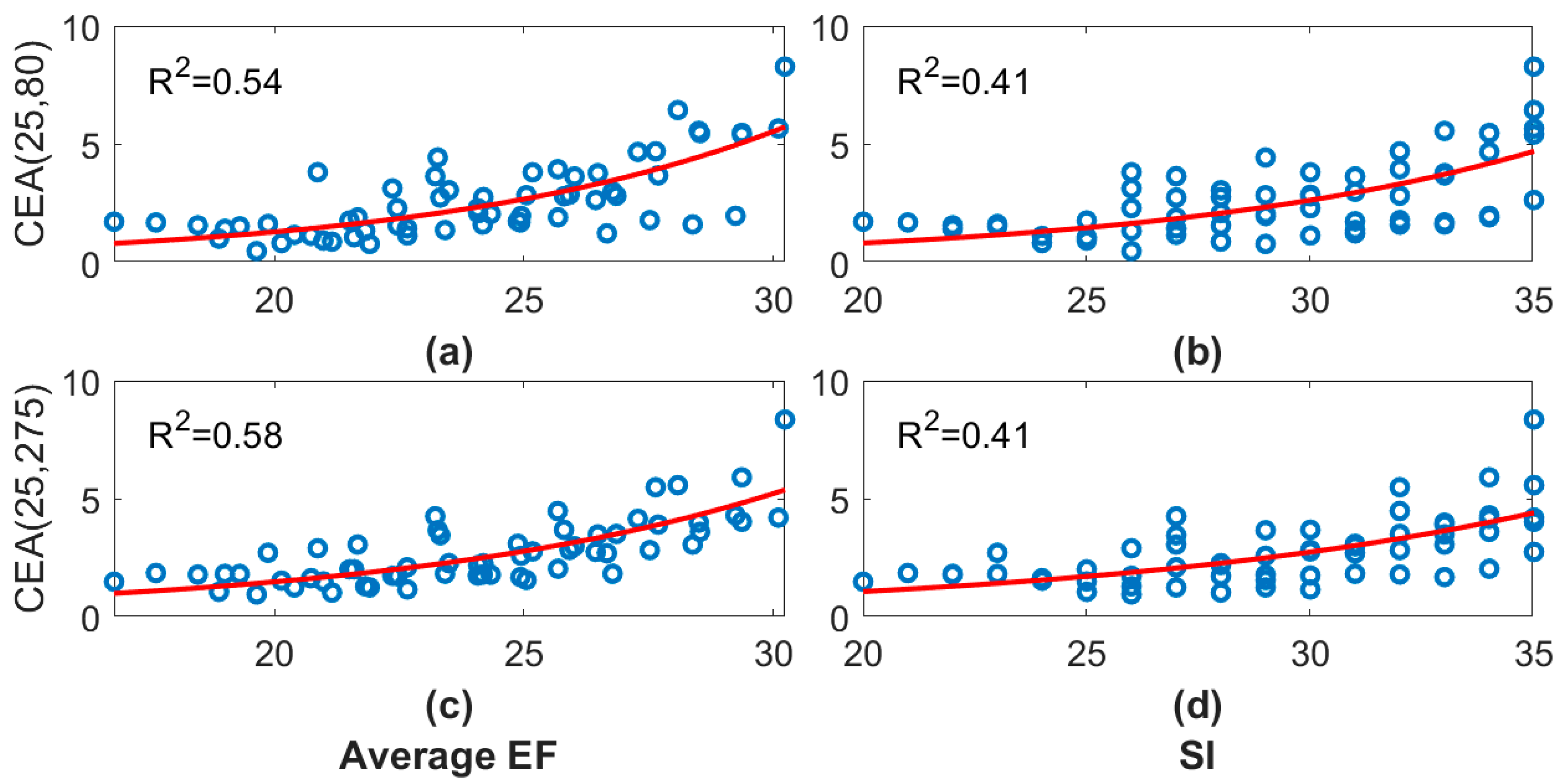
3.5. Relation of E-Field and Cortical Activity

The investigation of the relation between the intensity of the induced E-field and the cortical activity strength is performed by means of exponential model fits of TEP characteristics vs. the average field intensity over the whole brain. The TEP characteristics that are employed are the two CEA measures and the components described in Section 3.3. Figure 6 shows the model fits for the CEA measures for individual subjects, along with the adjusted $R^2$ value of the fit. We use a rule of thumb to assess the obtained values. We consider $R^2>0.7$ to correspond to very good fit, $0.3<R^2<0.7$ to moderate fit and $R^2<0.3$ to weak or no fit. Performing statistical tests for the significance of the adjusted $R^2$ is not appropriate in our case, due to the nonlinear fits, small sample size and non-normality of the data. Nonetheless, we tried statistical testing, and although the results are not very reliable, they were comparable to the ones from the rule of thumb (see Table S1). In $3$ out of the $5$ subjects (S2, S4, S5), there is a very good fit (adjusted $R^2~0.7$ to $0.9$), in 1 (S3), the fit is moderate ($R^2~0.4$ and $0.5$) and in 1 (S1) it is weak ($R^2~0.0$ and $0.3$). This last subject was the one with the highest LT and, as such, the bad fit could be explained by the fact that most of the points correspond to subthreshold intensities that do not produce TEPs. Linear fits produced much smaller $R^2$, with maximum value across all 10 cases being equal to 0.77 (see Figure S2). Although the number of points for each fit is rather small, the obtained adjusted $R^2$ values are evidence of the relation between the E-field intensity and cortical response strength and suggests that the relation is nonlinear and most probably of the exponential type.

In Figure 7, we present the model fit results for the pooled data of all subjects. Figure 7a,c show CEA(25,80) and CEA(25,275) vs. average E-field and produce $R^2$ of $0.54$ and $0.58$, respectively. As a comparison, we show in Figure 7b,d the exponential model fit for CEAs vs. the stimulation intensity (percentage of MSO). For both CEA cases, these fits produce markedly smaller $R^2$ at $0.41$. Linear fits here produced even smaller $R^2$ (more than $10\%$ reduction in all cases). It is conceivable that the relation form would probably be of a sigmoid type with midpoint the LT value, but our data would mostly correspond to the left part of the sigmoid curve, and thus, such a model fit would be problematic. Nonetheless, we attempted sigmoid fits, and the results did not change significantly compared to the exponential fit (see Table S2 for $R^2$ for the different fit types tested).

Finally, in Figure 8, we present the results of the model fits for the TEP components, as well as the amplitude difference of successively time ordered components. With the exception of the cases of P90-N75 and P110-N75 (Figure 8g,h), all other components show some degree of substantial model fit. With a rule of thumb for the threshold of acceptable $R^2$ equal to $0.5$, the cases of N75, N75-P60 and P150–N110 exhibit the best fits with $R^2=0.58, 0.63$ and $0.65$, respectively (we also note P150 which marginally does not cross the threshold of $0.5$, with $R^2=0.49$). It is interesting that the first two cases (N75 and N75-P60) correspond to early components, while the third (P150–N110) to late ones.

4. Discussion

The present study aims to elucidate, from a temporal and spatial point of view, the relation of the E-field induced by TMS stimulation and the ensuing electroencephalographic cortical response. We observed that post-TMS, there is an oscillating pattern in the correlation/covariance between the CSD/EEG and the E-field intensity as a function of latency, with alternating high correlation/anticorrelation periods. This implies the existence of an excitation–inhibition mechanism, which is triggered by the TMS administration and is correlated to the E-field distribution in the brain. With respect to the brain regions that were activated under our specific setup (stimulation with an H7 coil over the mid-central area and an SI of 120%LT), we show that cortical activation is essentially restricted near the stimulation locus and extends to a smaller area than the E-field. In essence, from the cortical neurons where a high E-field is induced, only a percentage is actually activated. This is in agreement with the theoretical considerations and results regarding the generation of cortical responses by TMS in [23].

To explore in detail the relation of TEPs and E-field for a wide range of sub- and suprathreshold stimulus intensities, we used exponential model fits and we observed moderate to substantially high adjusted $R^2$ values. This is clear evidence of the causal relation between TMS-induced E-fields and TEP generation. Furthermore, the fact that the $R^2$ values of linear model fits were smaller than those of the exponential model fits is evidence of the nonlinear nature of the relations in line with the theoretical considerations and experimental results in the pioneering study by Kommsi et al. [23].

From a practical point of view, it is important to note that the model fits of TEP characteristics vs. E-field provided higher $R^2$ than vs. the stimulation intensity. The superior fitting performance of E-fields should be ascribed to the fact that the E-field is a subject-specific parameter, whereas the stimulation intensity is not. The observation that the same intensity stimuli produce varying E-field distributions and varying cortical activation patterns in different subjects justifies the need for personalized analysis of TMS data. In clinical practice, the stimulation intensity is determined in a subject-specific manner (for instance, based on the motor threshold (MT) or on the basis of electroencephalographic criteria, such as the LT, when stimulating areas beyond the motor strip). However, it would be highly beneficial if the analysis was moved from the relatively arbitrary domain of stimulator intensity or even of a multiple of the MT/LT to a domain of physical meaning, such as the intensity of the induced E-field [53].

The results of the present study provide further physiological validation of the E-field modeling approach that is being increasingly employed for research and clinical purposes in the field of non-invasive brain stimulation. Previous studies, reviewed in Jose Gomez-Tames et al. in [31], explored the relation between E-field properties and motor cortex excitability, as reflected in the motor evoked potential (MEP) amplitude and active or resting motor threshold. For instance, Opitz et al. [22] reported a strong correlation ($0.70<r<0.91$) for the regression between the mean E-field in area M1 and MEP amplitude, whereas Mikkonen et al. [54] reported a significant correlation ($R^2=0.44$) between the E-field and resting MT. Our results extend these findings by correlating the E-field with individual TEP components as well as with the overall CEA in different time windows post-TMS. The advantage of employing TEPs for validating E-field models is that they constitute a more direct measure of cortical activation, compared to MEPs, and are applicable in every area of the cortical mantle, rather than being restricted to the motor strip.

Extensions of the work presented herein would be to move the analysis in the source space and/or expand the range of stimulation intensity values by including higher range supra-LT cases. This would allow for the more appropriate (intuitively) fitting of a sigmoid function, which in turn would lead to more meaningful extrapolations and better understanding of TMS-induced cortical activation. The promising results we report here need to be verified in a larger dataset. If so, they would constitute a further step that could lead to a paradigm shift toward the characterization of TMS on the basis of the induced E-field rather than on the stimulation intensity.

References

1. Rossini, P.M.; Burke, D.; Chen, R.; Cohen, L.G.; Daskalakis, Z.; Di Iorio, R.; Di Lazzaro, V.; Ferreri, F.; Fitzgerald, P.B.; George, M.S.; et al. Non-Invasive Electrical and Magnetic Stimulation of the Brain, Spinal Cord, Roots and Peripheral Nerves: Basic Principles and Procedures for Routine Clinical and Research Application. An Updated Report from an I.F.C.N. Committee. Clin. Neurophysiol. 2015, 126, 1071–1107. [Google Scholar] [CrossRef] [PubMed]
2. Kim, J.Y.; Chung, E.J.; Lee, W.Y.; Shin, H.Y.; Lee, G.H.; Choe, Y.-S.; Choi, Y.; Kim, B.J. Therapeutic effect of repetitive transcranial magnetic stimulation in Parkinson’s disease: Analysis of [11C] raclopride PET study. Mov. Disord. 2008, 23, 207–211. [Google Scholar] [CrossRef] [PubMed]
3. Kobayashi, M.; Pascual-Leone, A. Transcranial Magnetic Stimulation in Neurology. Lancet Neurol. 2003, 2, 145–156. [Google Scholar] [CrossRef]
4. Fitzgerald, P.B.; Brown, T.L.; Daskalakis, Z.J. The Application of Transcranial Magnetic Stimulation in Psychiatry and Neurosciences Research. Acta Psychiatr. Scand. 2002, 105, 324–340. [Google Scholar] [CrossRef]
5. Kimiskidis, V. Transcranial Magnetic Stimulation (TMS) Coupled with Electroencephalography (EEG): Biomarker of the Future. Rev. Neurol. 2016, 172, 123–126. [Google Scholar] [CrossRef]
6. Kimiskidis, V.; Tsimpiris, A.; Ryvlin, P.; Kalviainen, R.; Koutroumanidis, M.; Valentin, A.; Laskaris, N.; Kugiumtzis, D. TMS Combined with EEG in Genetic Generalized Epilepsy: A Phase II Diagnostic Accuracy Study. Clin. Neurophysiol. 2017, 128, 367–381. [Google Scholar] [CrossRef]
7. Vlachos, I.; Kugiumtzis, D.; Tsalikakis, D.G.; Kimiskidis, V.K. TMS-Induced Brain Connectivity Modulation in Genetic Generalized Epilepsy. Clin. Neurophysiol. 2022, 133, 83–93. [Google Scholar] [CrossRef]
8. Badawy, R.A.B.; Strigaro, G.; Cantello, R. TMS, Cortical Excitability and Epilepsy: The Clinical Impact. Epilepsy Res. 2014, 108, 153–161. [Google Scholar] [CrossRef]
9. Rotenberg, A. Prospects for Clinical Applications of Transcranial Magnetic Stimulation and Real-Time EEG in Epilepsy. Brain Topogr. 2010, 22, 257–266. [Google Scholar] [CrossRef]
10. Dimyan, M.A.; Cohen, L.G. Contribution of Transcranial Magnetic Stimulation to the Understanding of Functional Recovery Mechanisms after Stroke. Neurorehabil. Neural Repair 2010, 24, 125–135. [Google Scholar] [CrossRef] [Green Version]
11. D’Olhaberriague, L.; Gamissans, J.M.E.; Marrugat, J.; Valls, A.; Ley, C.O.; Seoane, J.L. Transcranial Magnetic Stimulation as a Prognostic Tool in Stroke. J. Neurol. Sci. 1997, 147, 73–80. [Google Scholar] [CrossRef]
12. Simpson, M.; Macdonell, R. The Use of Transcranial Magnetic Stimulation in Diagnosis, Prognostication and Treatment Evaluation in Multiple Sclerosis. Mult. Scler. Relat. Disord. 2015, 4, 430–436. [Google Scholar] [CrossRef] [PubMed]
13. Ferrazzano, G.; Crisafulli, S.G.; Baione, V.; Tartaglia, M.; Cortese, A.; Frontoni, M.; Altieri, M.; Pauri, F.; Millefiorini, E.; Conte, A. Early Diagnosis of Secondary Progressive Multiple Sclerosis: Focus on Fluid and Neurophysiological Biomarkers. J. Neurol. 2021, 268, 3626–3645. [Google Scholar] [CrossRef] [PubMed]
14. Weiler, M.; Stieger, K.C.; Long, J.M.; Rapp, P.R. Transcranial Magnetic Stimulation in Alzheimer’s Disease: Are We Ready? eNeuro 2019, 7, 0235-19.2019. [Google Scholar] [CrossRef]
15. Bagattini, C.; Mutanen, T.P.; Fracassi, C.; Manenti, R.; Cotelli, M.; Ilmoniemi, R.J.; Miniussi, C.; Bortoletto, M. Predicting Alzheimer’s Disease Severity by Means of TMS–EEG Coregistration. Neurobiol. Aging 2019, 80, 38–45. [Google Scholar] [CrossRef]
16. Laakso, I.; Murakami, T.; Hirata, A.; Ugawa, Y. Where and What TMS Activates: Experiments and Modeling. Brain Stimul. 2018, 11, 166–174. [Google Scholar] [CrossRef]
17. Bortoletto, M.; Veniero, D.; Thut, G.; Miniussi, C. The Contribution of TMS–EEG Coregistration in the Exploration of the Human Cortical Connectome. Neurosci. Biobehav. Rev. 2015, 49, 114–124. [Google Scholar] [CrossRef] [Green Version]
18. Tremblay, S.; Rogasch, N.C.; Premoli, I.; Blumberger, D.M.; Casarotto, S.; Chen, R.; Di Lazzaro, V.; Farzan, F.; Ferrarelli, F.; Fitzgerald, P.B.; et al. Clinical Utility and Prospective of TMS-EEG. Clin. Neurophysiol. 2019, 130, 802–844. [Google Scholar] [CrossRef]
19. Thielscher, A.; Kammer, T. Linking Physics with Physiology in TMS: A Sphere Field Model to Determine the Cortical Stimulation Site in TMS. Neuroimage 2002, 17, 1117–1130. [Google Scholar] [CrossRef] [Green Version]
20. Salminen-Vaparanta, N.; Koivisto, M.; Noreika, V.; Vanni, S.; Revonsuo, A. Neuronavigated Transcranial Magnetic Stimulation Suggests That Area V2 Is Necessary for Visual Awareness. Neuropsychologia 2012, 50, 1621–1627. [Google Scholar] [CrossRef]
21. Windhoff, M.; Opitz, A.; Thielscher, A. Electric Field Calculations in Brain Stimulation Based on Finite Elements: An Optimized Processing Pipeline for the Generation and Usage of Accurate Individual Head Models. Hum. Brain Mapp. 2013, 34, 923–935. [Google Scholar] [CrossRef] [PubMed]
22. Opitz, A.; Legon, W.; Rowlands, A.; Bickel, W.K.; Paulus, W.; Tyler, W.J. Physiological Observations Validate Finite Element Models for Estimating Subject-Specific Electric Field Distributions Induced by Transcranial Magnetic Stimulation of the Human Motor Cortex. Neuroimage 2013, 81, 253–264. [Google Scholar] [CrossRef] [PubMed] [Green Version]
23. Komssi, S.; Kähkönen, S.; Ilmoniemi, R.J. The Effect of Stimulus Intensity on Brain Responses Evoked by Transcranial Magnetic Stimulation. Hum. Brain Mapp. 2004, 21, 154–164. [Google Scholar] [CrossRef]
24. Deng, Z.-D.; Lisanby, S.H.; Peterchev, A.V. Coil Design Considerations for Deep Transcranial Magnetic Stimulation. Clin. Neurophysiol. 2014, 125, 1202–1212. [Google Scholar] [CrossRef] [Green Version]
25. Parazzini, M.; Fiocchi, S.; Chiaramello, E.; Roth, Y.; Zangen, A.; Ravazzani, P. Electric Field Estimation of Deep Transcranial Magnetic Stimulation Clinically Used for the Treatment of Neuropsychiatric Disorders in Anatomical Head Models. Med. Eng. Phys. 2017, 43, 30–38. [Google Scholar] [CrossRef] [PubMed]
26. Afuwape, O.F.; Rastogi, P.; Jiles, D.C. Comparison of the Effect of Coil Configuration and the Variability of Anatomical Structure on Transcranial Magnetic Stimulation. IEEE Trans. Magn. 2021, 57, 1–5. [Google Scholar] [CrossRef]
27. Nieminen, J.O.; Koponen, L.M.; Ilmoniemi, R.J. Experimental Characterization of the Electric Field Distribution Induced by TMS Devices. Brain Stimul. 2015, 8, 582–589. [Google Scholar] [CrossRef] [PubMed]
28. Gomez, L.J.; Yücel, A.C.; Hernandez-Garcia, L.; Taylor, S.F.; Michielssen, E. Uncertainty Quantification in Transcranial Magnetic Stimulation via High-Dimensional Model Representation. IEEE Trans. Biomed. Eng. 2015, 62, 361–372. [Google Scholar] [CrossRef]
29. Janssen, A.M.; Oostendorp, T.F.; Stegeman, D.F. The Coil Orientation Dependency of the Electric Field Induced by TMS for M1 and Other Brain Areas. J. Neuroeng. Rehabil. 2015, 12, 47. [Google Scholar] [CrossRef] [Green Version]
30. Konakanchi, D.; de Jongh Curry, A.L.; Waters, R.S.; Narayana, S. Focality of the Induced E-Field Is a Contributing Factor in the Choice of TMS Parameters: Evidence from a 3D Computational Model of the Human Brain. Brain Sci. 2020, 10, 1010. [Google Scholar] [CrossRef]
31. Gomez-Tames, J.; Laakso, I.; Hirata, A. Review on Biophysical Modelling and Simulation Studies for Transcranial Magnetic Stimulation. Phys. Med. Biol. Biol. 2020, 65, 24TR03. [Google Scholar] [CrossRef] [PubMed]
32. Carmi, L.; Tendler, A.; Bystritsky, A.; Hollander, E.; Blumberger, D.M.; Daskalakis, J.; Ward, H.; Lapidus, K.; Goodman, W.; Casuto, L.; et al. Efficacy and Safety of Deep Transcranial Magnetic Stimulation for Obsessive-Compulsive Disorder: A Prospective Multicenter Randomized Double-Blind Placebo-Controlled Trial. Am. J. Psychiatry 2019, 176, 931–938. [Google Scholar] [CrossRef] [PubMed]
33. Roth, Y.; Amir, A.; Levkovitz, Y.; Zangen, A. Three-Dimensional Distribution of the Electric Field Induced in the Brain by Transcranial Magnetic Stimulation Using Figure-8 and Deep H-Coils. J. Clin. Neurophysiol. 2007, 24, 31–38. [Google Scholar] [CrossRef] [PubMed]
34. Levkovitz, Y.; Roth, Y.; Harel, E.V.; Braw, Y.; Sheer, A.; Zangen, A. A Randomized Controlled Feasibility and Safety Study of Deep Transcranial Magnetic Stimulation. Clin. Neurophysiol. 2007, 118, 2730–2744. [Google Scholar] [CrossRef] [PubMed]
35. Levkovitz, Y.; Harel, E.V.; Roth, Y.; Braw, Y.; Most, D.; Katz, L.N.; Sheer, A.; Gersner, R.; Zangen, A. Deep Transcranial Magnetic Stimulation over the Prefrontal Cortex: Evaluation of Antidepressant and Cognitive Effects in Depressive Patients. Brain Stimul. 2009, 2, 188–200. [Google Scholar] [CrossRef]
36. Isserles, M.; Rosenberg, O.; Dannon, P.; Levkovitz, Y.; Kotler, M.; Deutsch, F.; Lerer, B.; Zangen, A. Cognitive–Emotional Reactivation during Deep Transcranial Magnetic Stimulation over the Prefrontal Cortex of Depressive Patients Affects Antidepressant Outcome. J. Affect. Disord. 2011, 128, 235–242. [Google Scholar] [CrossRef]
37. Virtanen, J.; Ruohonen, J.; Näätänen, R.; Ilmoniemi, R.J. Instrumentation for the Measurement of Electric Brain Responses to Transcranial Magnetic Stimulation. Med. Biol. Eng. Comput. 1999, 37, 322–326. [Google Scholar] [CrossRef]
38. Wagner, T.A.; Zahn, M.; Grodzinsky, A.J.; Pascual-Leone, A. Three-Dimensional Head Model Simulation of Transcranial Magnetic Stimulation. IEEE Trans. Biomed. Eng. 2004, 51, 1586–1598. [Google Scholar] [CrossRef]
39. Fiocchi, S.; Longhi, M.; Ravazzani, P.; Roth, Y.; Zangen, A.; Parazzini, M. Modelling of the Electric Field Distribution in Deep Transcranial Magnetic Stimulation in the Adolescence, in the Adulthood, and in the Old Age. Comput. Math. Methods Med. 2016, 2016, 9039613. [Google Scholar] [CrossRef] [Green Version]
40. Samoudi, A.M.; Tanghe, E.; Martens, L.; Joseph, W. Deep Transcranial Magnetic Stimulation: Improved Coil Design and Assessment of the Induced Fields Using MIDA Model. BioMed Res. Int. 2018, 2018, 7061420. [Google Scholar] [CrossRef]
41. Herring, J.D.; Thut, G.; Jensen, O.; Bergmann, T.O. Attention Modulates TMS-Locked Alpha Oscillations in the Visual Cortex. J. Neurosci. 2015, 35, 14435–14447. [Google Scholar] [CrossRef] [PubMed] [Green Version]
42. He, P.; Wilson, G.; Russell, C. Removal of Ocular Artifacts from Electro-Encephalogram by Adaptive Filtering. Med. Biol. Eng. Comput. 2004, 24, 407–412. [Google Scholar] [CrossRef] [PubMed]
43. Mitra, P.; Bokil, H. Observed Brain Dynamics; Oxford University Press: Oxford, UK, 2007; ISBN 9780199864829. [Google Scholar]
44. Kothe, C.A.; Makeig, S. BCILAB: A Platform for Brain-Computer Interface Development. J. Neural Eng. 2013, 10, 056014. [Google Scholar] [CrossRef] [PubMed] [Green Version]
45. Mullen, T.R.; Kothe, C.A.E.; Chi, Y.M.; Ojeda, A.; Kerth, T.; Makeig, S.; Jung, T.P.; Cauwenberghs, G. Real-Time Neuroimaging and Cognitive Monitoring Using Wearable Dry EEG. IEEE Trans. Biomed. Eng. 2015, 62, 2553–2567. [Google Scholar] [CrossRef] [PubMed] [Green Version]
46. Rogasch, N.C.; Sullivan, C.; Thomson, R.H.; Rose, N.S.; Bailey, N.W.; Fitzgerald, P.B.; Farzan, F.; Hernandez-Pavon, J.C. Analysing Concurrent Transcranial Magnetic Stimulation and Electroencephalographic Data: A Review and Introduction to the Open-Source TESA Software. Neuroimage 2017, 147, 934–951. [Google Scholar] [CrossRef] [PubMed]
47. Kayser, J.; Tenke, C.E. Principal Components Analysis of Laplacian Waveforms as a Generic Method for Identifying ERP Generator Patterns: II. Adequacy of Low-Density Estimates. Clin. Neurophysiol. 2006, 117, 369–380. [Google Scholar] [CrossRef]
48. Kayser, J.; Tenke, C.E. Principal Components Analysis of Laplacian Waveforms as a Generic Method for Identifying ERP Generator Patterns: I. Evaluation with Auditory Oddball Tasks. Clin. Neurophysiol. 2006, 117, 348–368. [Google Scholar] [CrossRef]
49. Kayser, J.; Tenke, C.E. On the Benefits of Using Surface Laplacian (Current Source Density) Methodology in Electrophysiology. Int. J. Psychophysiol. 2015, 97, 171–173. [Google Scholar] [CrossRef] [Green Version]
50. Rosanova, M.; Sarasso, S.; Massimini, M.; Casarotto, S. Cortical Excitability, Plasticity and Oscillations in Major Psychiatric Disorders: A Neuronavigated TMS-EEG Based Approach. In Non Invasive Brain Stimulation in Psychiatry and Clinical Neurosciences; Dell’Osso, B., Di Lorenzo, G., Eds.; Springer: Cham, Switzerland, 2020; pp. 209–222. [Google Scholar]
51. Rajji, T.K.; Sun, Y.; Zomorrodi-Moghaddam, R.; Farzan, F.; Blumberger, D.M.; Mulsant, B.H.; Fitzgerald, P.B.; Daskalakis, Z.J. PAS-Induced Potentiation of Cortical-Evoked Activity in the Dorsolateral Prefrontal Cortex. Neuropsychopharmacol 2013, 38, 2545–2552. [Google Scholar] [CrossRef] [Green Version]
52. Delorme, A.; Makeig, S. EEGLAB: An Open Source Toolbox for Analysis of Single-Trial EEG Dynamics Including Independent Component Analysis. J. Neurosci. Methods 2004, 134, 9–21. [Google Scholar] [CrossRef] [Green Version]
53. Rosanova, M.; Casali, A.; Bellina, V.; Resta, F.; Mariotti, M.; Massimini, M. Natural Frequencies of Human Corticothalamic Circuits. J. Neurosci. 2009, 29, 7679–7685. [Google Scholar] [CrossRef] [PubMed]
54. Mikkonen, M.; Laakso, I.; Sumiya, M.; Koyama, S.; Hirata, A.; Tanaka, S. TMS Motor Thresholds Correlate with TDCS Electric Field Strengths in Hand Motor Area. Front. Neurosci. 2018, 12, 426. [Google Scholar] [CrossRef] [PubMed] [Green Version]
Figure 1. E-fields for all subjects. Warm colors indicate high values, while cold indicate low values. The color scale is not consistent across subjects for visualization purposes.
Applsci 12 07437 g001
Figure 2. (a) Average TEP across subjects on top and GFP on bottom, (b) Correlation ρ of CSD and E-field values for all subjects on top and their average on bottom, (c) same as (b), for covariance σ .
Applsci 12 07437 g002
Figure 3. Topographic plots of the E-field, and CEA(25,80) and CEA(25,275) (rows) for all subjects (columns), as indicated on the top and left.
Applsci 12 07437 g003
Figure 4. Topographic plots for the average across all subjects E-field, and CEA(25,80) and CEA(25,275), as well as indicative CEA values for two pre-TMS windows.
Applsci 12 07437 g004
Figure 5. (a) ROI-averaged TEPs for the ROI of nine central channels and for individual subject, and (b) the average across subjects TEP, along with identified components.
Applsci 12 07437 g005
Figure 6. Exponential model fits for the CEA measure vs. the average E-field for each subject separately. (ae) correspond to subjects S1-S5, as indicated by the inset text. Top panels are for CEA(25,80) and bottom panels for CEA(25,275). The adjusted R 2 for each model fit is shown inside each panel.
Applsci 12 07437 g006
Figure 7. Exponential model fits for the CEA(25,80) measure across all subjects vs. (a) the average E-field and (b) the stimulation intensity. (c,d) are the same as (a,b), but for CEA(25,275). The adjusted R 2 for each model fit is shown inside each panel.
Applsci 12 07437 g007
Figure 8. (ae) Exponential model fits of the TEP components vs. the average E-field value, and the difference of successive components values (fi). The adjusted R2 for each model fit is shown inside each panel.
Applsci 12 07437 g008