Article

Study on Noise Model of an Automotive Axial Fan Based on Aerodynamic Load Force

1
College of Mechanical and Vehicle Engineering, Chongqing University, Chongqing 400044, China
2
Dongfeng Xiaokang Automobile Co., Ltd., Chongqing 402260, China
*
Author to whom correspondence should be addressed.
Appl. Sci. 2022, 12(14), 7326; https://doi.org/10.3390/app12147326
Submission received: 27 April 2022 / Revised: 8 July 2022 / Accepted: 13 July 2022 / Published: 21 July 2022
(This article belongs to the Section Mechanical Engineering)

Abstract

:
Due to the fact that the noise caused by axial fan blades of vehicles is large, which seriously affects ride comfort, and there is no effective mathematical model to quantitatively study the contribution of the various parameters of the blades to the noise, a new method for calculating the load force of the blades is proposed. This method obtains the constant load force of the blade according to the blade element momentum theory and the characteristics of the blade structure of the axial fan for a vehicle. At the same time, this method obtains the non-constant load force of the blade by combining the non-constant thin-wing theory and experimental data and then vectors the constant load force and the non-constant load force to obtain the total load force of the blade to build a mathematical model of the relationship between the noise of the fan and the parameters of the blade. According to the model, the total sound pressure level of a fan is calculated numerically and further compared with the FLUENT software simulation and experimental results. The results show that the error of the total sound pressure level calculated by the numerical value is within 3 dB(A). This method provides an important basis for the study of a high-accuracy noise mathematical model and the optimization of blade parameters of low Mach-number fans.

1. Introduction

Vehicle axial cooling fans are frequently used to provide enough air through heat exchangers (radiators) to control engine temperature even at low vehicle speeds or in idle conditions [1]. As the core part of the cooling system, the operating noise of the fan greatly affects the ride comfort of the vehicle. Modern vehicles generally use axial flow cooling fans, and the fan noise includes aerodynamic noise, pipe radiation noise, and motor and casing noise, and among these types of noise, aerodynamic noise is the loudest [2]. Aerodynamic noise is generated by the noise caused by flow [3] and consists mainly of two parts, namely broadband noise and discrete noise. Existing studies have shown that the sound pressure pulsations generated by the periodic impacting of the blade wake flow on downstream objects are superimposed on the fundamental and harmonic frequencies of the blade pulsations, so that the sound pressure level of discrete noise is much higher than that of broadband noise [4].
In order to calculate the aerodynamic noise of the fan, the load noise of the fan must be calculated [5]. The load noise is related to the load force on the surface of the fan blade. For the determination of the load force of wind turbine blades, many scholars have conducted research. Under the conditions of a low Mach number, the noise of the rotary airfoil blade is mainly dipole noise, that is, load noise that is related to the load force on the surface of fan blades [6]. Sun [7] pointed out that the aerodynamic noise of the rotating blade is mainly generated by the pulsating pressure distributed on both sides of the blade. Zuo [8] used a 3D CFD model to simulate and analyze the internal flow field of a vortex fan, obtained the pressure pulsation information on the blade surface, used the pressure flow field of the blade surface as the aerodynamic sound source, and calculated the far field aerodynamic noise generated by the blade by solving the FW-H equation. The calculation results showed that the aerodynamic noise of the blade thickness was from 1 mm to 4 mm in the thin-wing range and its aerodynamic noise was dominant compared with the structured noise and remained basically unchanged. The constant load force of the blade can be obtained by the blade element momentum (BEM) theory through which the blade can be divided into many small units and the constant load force of each unit can be related to parameters such as inflow velocity, chord length, and installation angle through the momentum so as to facilitate the calculation of far-field noise using the FW-H equation [9]. Zeng [10] used BEM theory to solve the relative inflow velocity and inflow angle of attack of each blade element in a blade wind turbine, and each position corresponded to different airfoil parameters such as velocity, angle of attack, and chord length, which are necessary input parameters for airfoil noise calculation. Zheng [11] obtained the lift and resistance characteristic data of an automotive axial flow fan using the table lookup method from the inflow speed to obtain the constant load force. Based on BEM theory, Qian [12] used the lift and resistance characteristic data of a wind turbine, as well as the constant aerodynamic load force, including chord length and installation angle, which was obtained from the inflow velocity, and then the FW-H equation was used to establish a prediction model of the rotating blade noise of a wind turbine. Liu [13] pointed out that axial fan blades need to withstand complex aerodynamic loads in addition to constant forces but did not give a clear expression. The influencing factors of low-pressure axial flow fan noise are mainly divided into three aspects: thickness noise, constant-force noise, and non-constant-force noise; The aerodynamic force on the blade surface is highly unsteady and the uneven inlet interacts with the impeller producing a strong unsteady pulsation on the blade surface, thereby radiating noise, and the non-constant-force noise is the main discrete noise source of a low-pressure axial flow fan [14]. The experimental study in [15] shows that the influence of the Reynolds number (Re for short) on acoustic radiation is implicit in the unsteady force and that discrete sound plays a dominant role in the non-self-mode region with a low Re number, whereas the automotive axial flow fan is in the low Re number non-self-mode region. Due to the complexity of the load force on the fan blade, none of the above studies have obtained an accurate load force.
In this paper, a new method based on previous studies is proposed and successfully applied to the axial flow fan of a vehicle. First, the relationships between the lift, resistance characteristics, and the angle of attack are established according to the BEM theory and the characteristics of the axial flow fan blades of the vehicle, and the constant force is obtained. Then, the relationship between unsteady lift and velocity using the unsteady thin-wing theory is established and the non-constant force is obtained. The constant and non-constant forces of each microelement are obtained using vector superposition to obtain the total load force. This method provides an important basis for the study of a high-precision noise mathematical model of a low Mach-number fan.

2. Establishment of Axial Fan Blade Loading Force

In order to calculate the noise of the fan, the loading noise of the fan must be calculated. The loading noise is related to the loading force on the fan blade surface. Blade surface loading force is usually divided into steady force and unsteady force, which can be obtained using the N-S equation. The N-S equation is a nonlinear implicit equation and the relationship between the loading force and the fan blade structure and aerodynamic performance parameters cannot be obtained. In this paper, the relationship between the steady loading force and fan inlet velocity, installation angle, and other parameters is established based on the BEM theory. Based on the unsteady thin-wing theory and experimental data, the relationship between the unsteady loading force, pulsation velocity, and inflow angle is established. Then, the relationship between the unsteady loading force, inflow velocity of the fan, and blade installation angle is established. The relationship between the loading force and blade chord length is established using the theory of blade chord load distribution and the complete loading force model of the blade is obtained.

2.1. BEM Theory

Blade element theory assumes that the blade can be divided into many elements along the radius direction and each element is relatively independent of the other, which can be regarded as a two-dimensional model. In this way, the aerodynamic force on each element is calculated based on the local flow conditions. Then, the aerodynamic force on each element along the radius direction is integrated and the total aerodynamic force is calculated. The momentum theory assumes that the pressure or momentum loss on the rotor plane is caused by the flow through the blade element. Each blade element segment connects tangential velocity with tangential force through the conservation of the circumferential moment of momentum and connects axial velocity with axial force using the momentum theorem. The combination of the blade element theory and momentum theory embodies the BEM theory.
According to the classical blade element theory, the flow tube section is discretized into several annular elements with a height of dr. For ring elements, the assumptions are as follows: (1) The radial properties of ring elements are independent; and (2) In each ring element, the force exerted by the blade on the flow is constant. In view of this, in a flow tube with radius r and width dr, the mass flow rate of air is
d m ˙ = ρ v dA = 2 π ρ v r d r
The pull force dT on the control body is
d T = ( v 1 v 0 ) d m ˙ = 4 π ρ v 2 r d r
In the cooling fan, the motor drives the blade to rotate and accelerate the air and the moment of air on the blade is the resistance moment. Using the moment of momentum theorem, the torque dM in the d r flow tube can be written as
d M = ( ω 1 r ω 0 r ) r d m ˙ = 4 π ρ v ω f r 3 d r
In the formula, ω f is the circumferential induced angular velocity of the fan blade rotation plane.

2.2. Steady Force

Figure 1 shows the force diagram at a certain section of the fan blade element. It can be seen in Figure 1 that θ is the installation angle of the blade element and α and φ are the airfoil attack angle and the inlet angle, respectively. In the blade element (airfoil) rotation plane, the relationship between relative velocity v r e l , axial-induced velocity v of air, annular-induced angular velocity ω f , blade rotation angular velocity ω F A N , and the inlet angle φ is
v r e l = v 2 + ( ω F A N ω f ) 2 r 2
tan φ = v ( ω F A N ω f ) r
The blade installation angle is
θ = φ + α
where α is the attack angle.
The lift force L and resistance D are constant forces and the lift force L and resistance D per unit length are, respectively,
L = 1 2 ρ v r e l 2 c h C L
D = 1 2 ρ v r e l 2 c h C D
where ch is the chord length of the airfoil, CL is the lift coefficient, and CD is the resistance coefficient.
Based on the LS blade profile lift resistance coefficient and the blade profile size of existing automotive fans, the relationships between the lift coefficient CL, resistance coefficient CD, and attack angle are as follows:
C L = 0.5 + 0.08 ( α 4 )
C D = 0.5 + 0.08 ( α 4 ) 0.116071 α 4 + 0.407738 α 3 + 0.5625 α 2 + 14.592262 α + 14.553571
Since only the vertical and tangential forces in the blade rotation plane are focused on, the lift force and resistance are projected in these directions, as shown in Figure 1.
F N = L c o s φ D s i n φ
F T = L s i n φ + D c o s φ
According to Equations (2), (3), (11), and (12) and combined with momentum theory, the following equations can be obtained:
8 π v 2 r = B c h v r e l 2 ( C L c o s φ C D s i n φ )
8 π v ω f r 2 = B c h v r e l 2 ( C L s i n φ + C D c o s φ )
The limitation of the BEM theory is that it does not consider the influence of tip vortices. At present, the Blount tip loss model is widely used to modify blade tip loss based on the BEM theory. In this model, the blade tip loss factor Lf is used to modify the induced velocity field, as shown in Equation (15) [12]:
C F = 2 π arccos ( e f ω )
where f ω = B 2 ( R r r s i n φ ) .
Then, Equations (13) and (14) are, respectively, expressed as
8 π v 2 r C F = B c h v r e l 2 ( C L c o s φ C D s i n φ )
8 π v ω f r 2 C F = B c h v r e l 2 ( C L s i n φ + C D c o s φ )
Based on the condition that the installation angle θ and chord length ch are known, the axial-induced velocity ν, annular-induced angular velocity ω f , and α of air can be calculated by combining Equations (16) and (17), thus the steady force FN and FT can be obtained.

2.3. Unsteady Forces

Since the unsteady force is caused by the velocity pulsation near the blade surface, it is assumed that the average flow through the wing is a constant Ur and the disturbance velocity is a small quantity U = [ U 1 ,   U 2 ,   U 3 ] , so it can be obtained by ignoring the square term of a small quantity:
C L C L ¯ + C L α α + C L γ γ = C L ¯ + C L α U 2 U r + C L γ U 3 U r
C D C D ¯ + C D α U 2 U r + C D γ U 3 U r
where C L ¯ and C D ¯ are the time-averaged lift and resistance coefficients, respectively. The slopes of lift and resistance are taken as constants. According to Equations (7) and (8), the perturbation lift per unit length along the blade height is L = L L ¯ and the resistance is D = D D ¯ , respectively.
L = 1 2 ρ c h U r ( C L α U 2 + C L γ U 3 + 2 C L ¯ U 1 )
D = 1 2 ρ c h U r ( C D α U 2 + C D γ U 3 + 2 C D ¯ U 1 )
As the resistance coefficient CD is much smaller than the lift coefficient CL under the thin wing, the pulsating resistance D is much smaller than the pulsating lift force L and can be ignored. The slope of the theoretical lift line C L α for a two-dimensional thin wing with a low attack angle α is equal to 2 π . Because of a two-dimensional inlet wind U = [ U 1 ,   U 2 ,   0 ] , the disturbance lift formed is therefore given as
L c h = ρ π U r U 2 + 2 ρ π α U 1
where the second term can be ignored compared with the first term when the attack angle α is small. So, there is
L c h = ρ π U r U 2
where the lift disturbance acting on such a blade is only caused by the attack angle disturbance caused by the change in velocity U 2 . The magnitude of U 2 is denoted by. The magnitude of ν is denoted by v A . The relationship between U 2 A and v A is as follows [16]:
U 2 A = 0.04 v A
where, A represents the amplitude.
The Sears function is used to calculate the blade pulsating lift force per unit length (along the radius direction) [17]:
f n = π c h ρ U r U 2 A c o s φ e i n ω F A N τ S c ( σ n ,   M r )
where n represents the n order harmonic wave and the pulse dynamic amplitude is
f n A = π c h ρ U r U 2 A c o s φ S c ( σ n ,   M r )
where the equivalent frequency σ n is
σ n = n ω F A N c h 2 U r
Equation (25) shows that the lift force acting on the blade is a periodic function of time, the fundamental frequency corresponds to the blade speed, and the n order harmonic only depends on the n order spatial harmonic component of the incoming flow disturbance field.
S c ( σ n ,   M r ) = s ( σ n / β r 2 ) β r [ J 0 ( M r 2 σ n β r 2 ) + i J 1 ( M r 2 σ n β r 2 ) ] e i σ n f ( M r ) β r 2
where s represents the Sears function. s ( σ n / β r 2 ) = e i σ n / β r 2 [ 1 π 2 2 ( 1 + 2 π σ n / β r 2 ) ] 1 + 2 π σ n / β r 2 ,   β r = 1 M r 2 , M r = U r c 0 , f ( M r ) = ( 1 β r ) ln M r + β r ln ( 1 + β r ) ln 2 ,   J 0 and J 1 is the Bezier function.
According to the Fourier transform, the amplitude coefficient of all harmonics is the amplitude relationship between the n order harmonics and the n − 1 order harmonics (n − 1)/n. It can be seen that the order is higher and the amplitude is accordingly lower. In this paper, the unsteady force L F is calculated and analyzed mainly from the first six-order unsteady force causing the blade pulsation noise.
L F = n = 1 6 f n

2.4. The Loading Force Varies with the Chord Length of the Blade

From the above-steady and unsteady forces, the blade loading force Fr can be obtained by vector superposition, which is the load force distribution along the radius direction. Based on the above, the distribution of the loading force along the chord length is studied. In order to reduce the calculation time, the influence of the airfoil thickness is ignored, the upper and lower surface elements are synthesized into a single element, and the pressure value is adopted by the pressure difference between the upper and lower surface elements [18]. For the inclined parabolic load, the fan’s circumferential load distribution is shown in Figure 2 in the blade coordinate system. Here, θ* represents the azimuth in the blade coordinate system and b is the chord length of the blade element at r .
According to the literature [7], the actual distribution of the chord load of the blade element is closest to the assumption of the inclined parabolic shape, so in the numerical calculation of loading noise in this paper, the load of the inclined parabolic shape distribution is selected to calculate the chord distribution of the aerodynamic load on the blade element.
The load distribution function is
l ( θ * ) = { 1.5 F r b 1.35 F r r 2 b 3 ( θ * ) 2 , b 3 r θ * 0 1.5 F r b 1.35 F r r 2 4 b 3 ( θ * ) 2 ,   0 θ * 2 b 3 r
where l is the blade loading force.

3. Noise Model of Automotive Axial Fan

Based on the steady and unsteady loading forces on the blade surface of the axial fan combined with the FW-H equation, the noise mathematical model including the parameters of the automotive axial fan is established, and then the time–domain solution of the noise model is obtained through the coordinate transformation and delay equation.

3.1. Establishment of Fan Mathematical Model Noise

The FW-H equation is the basic equation of aeroacoustics. Assuming that the control surface f ( x i ,   t ) = 0 is the fan blade surface, the most commonly used form of the FW-H equation can be obtained:
( 1 c 2 2 t 2 2 x i 2 ) p ( x i ,   t ) = [ ρ 0 v n δ ( f ) ] t [ F i δ ( f ) ] x i + 2 [ T i j H ( f ) ] x i x j
In the formula, 1 c 2 2 t 2 2 x i 2 is the operator for volatility, p(xi, t) represents the sound pressure value of the observation point at time t, v n = f t represents the outside normal vector of the control surface velocity, F i = P i j · n j is the blade surface load component, and the far right term represents the thickness sound source, load sound source, and quadrupole sound source, respectively. T i j = ρ u i u j P i j c 2 ρ δ i j is the Lighthill stress tensor. ρ and P i j are the density and stress tensors, respectively. δ i j is Kronecker symbol; subscript 0 represents undisturbed quantity; the apostrophe denotes perturbations; n represents the projection of control surface normal; H ( f ) is the Heaviside function; and δ ( f ) represents Dirac and satisfies
H ( f ) = { 0   f ( x i ,   t ) < 0 1   f ( x i ,   t ) > 0   ,   δ ( f ) = x = H ( f ) f
The automotive axial fan is at low speed and subsonic flow, so the quadrupole noise can be ignored. Assuming that the volume density is constant, the non-equilibrium mass flow into the fluid is equivalent to a monopole, which can be ignored. In this case, the FW-H equation can be expressed as
( 1 c 2 2 t 2 2 x i 2 ) p ( x i ,   t ) = [ ρ 0 v n δ ( f ) ] t [ F i δ ( f ) ] x i
It is assumed that the fan blades are in constant motion. In fan blade noise calculated by the application of delay time, the integrand function of each sound source on the blade surface f = 0 is adopted using the appropriate value corresponding to the respective delay time τ , namely the acoustic pressure p(x, t), the sound blade surface microelements in their respective corresponding delay time τ emissions, and the sum of the acoustic signals of the same receiving points in X.
According to FW-H Equation (33), the time–domain calculation formula of noise is
p ( x ,   t ) = 1 4 π f = 0 [ ρ 0 V n ( r M ˙ i r i ^ + c 0 M r c 0 M 2 ) r 2 ( 1 M r ) 3 ] r e t d s + 1 4 π c 0   f = 0 [ l ˙ i r ^ i r ( 1 M r ) 2 ] r e t d s + 1 4 π f = 0 [ l r l i M i r 2 ( 1 M r ) 2 ] r e t d s   + 1 4 π c 0   f = 0 [ l r ( r M ˙ i r ^ i + c 0 M r c 0 M 2 ) r 2 ( 1 M r ) 3 ] r e t d s
In the formula, the first term is the thickness noise, the second, third, and fourth terms are the load noise, and “ret” stands for the delay time. ρ 0 is the air density, and c0 is the sound velocity. Vi is the velocity component of the particle velocity fixed on the surface along the xi axis and the subscript i represents the component along the x i axis. V n = V i n i is the normal velocity of the moving elements along the physical plane and ni is the normal vector of the elements. V ˙ n is the derivative of the normal velocity of the moving elements along the physical plane with time. r is the distance of the sound source on the blade surface to the receiving point. r ^ = e i r ^ i is the unit vector for the receiver radiation direction, r ^ i = ( x i y i ) / r is the component of the vector r ^ on the xi axis and among them, r = ( x i y i ) 2 . M i = V i / c 0 is the Mach number of the moving microelement. Assuming that M r = V i r ^ i / c 0 is the projection of the Mach number of the moving microelement onto the R ^   vector, l is the loading force of the microelement on the blade surface and li is the component of the force l in the direction of the xi axis. lr is the projection of l at the receiving point direction and l ˙ i is the derivative of the load with respect to the time τ. The location of the receiving point in this paper is one meter in the leeward direction of the center point of the fan. The noise of Equation (34) is discretized in space, that is, the fan blade is divided into many tiny sound source surfaces Δs, and the fan noise can be obtained as follows:
p ( x ,   t ) = 1 4 π j = 1 m [ ρ 0 V n ( r M ˙ i R ^ i + c 0 M r c 0 M 2 ) r 2 ( 1 M R ) 3 ] ret · Δ s j + 1 4 π j = 1 m { [ l ˙ i R ^ i c 0 R ( 1 M R ) 2 + l R l i M i R 2 ( 1 M R ) 2 + l R ( R M ˙ i R ^ i + c 0 M R c 0 M 2 ) c 0 R 2 ( 1 M R ) 3 ] r e t } · Δ s j
where the sound source surface Δsj represents the jth microsound source surface, j = 1, …, m. m means that the whole sound source is divided into m microsource surfaces.
The total sound pressure p ( t ) at time t is obtained using a numerical calculation based on Equation (36). For the discretization of time t, the sampling time interval of each point is 0.0001 s and the discrete time t can be expressed as
t ( i ) = 0.0001 × ( i 1 )
where i = 1, …, k. In order to perform the FFT calculation, the number of sampling points k must be an exponent of 2. In consideration of accuracy and computing resources, k should be 256.
The effective value of the total sound pressure within a period (expressed in dB) is [19]
S = 10 log 10 i = 1 k p ( i ) 2 k × 0.00002 2
where p(i) represents the sound pressure corresponding to time t(i).

3.2. Time–Domain Solution of Fan Noise Model

The position of each point on the blade is in the blade coordinate system, whereas the receiving point is in the fixed coordinate system. In order to describe the distance between them, the position of each point source must be transformed from the blade coordinate system to the fixed coordinate system, including the conversion between the blade coordinate system and the rotating coordinate system, and the rotation coordinate system and the ground coordinate system.
The fan blade movement produces a pressure disturbance in the fluid (air) and forms aerodynamic noise. The aerodynamic noise of the fan is the result of the superposition of sound waves radiating from all points on the surface of the fan blade. The sound pressure at the receiving point is the sum of all pressure waves emitted by all sound sources at different times but arriving at the same receiving point at the same time, so it needs to be solved by the delay equation.

3.2.1. Coordinate Conversion

Assuming that the position of a point source on the blade surface in the blade coordinate system is ξ = ( a ,   b ,   c ) T , the position of the point source in the fixed coordinate system can be described by the coordinate transformation formula [6]:
y = [ 1 0 0 0 cos θ sin θ 0 sin θ cos θ ] [ a b c ] + [ 0 0 h ]
where y is the position vector of the point source on the blade surface in the fixed coordinate system.
The coordinate of the receiving point is described as x = ( x 1 ,   x 2 ,   x 3 ) T and combined with Equation (38), the radiation vector can be written as
r = x y = [ x 1 a x 2 b cos θ + c sin θ x 3 b sin θ c cos θ h ] = [ r 1 r 2 r 3 ]

3.2.2. Time–Domain Solution of Delay Equation

In the fan blade noise model, it is necessary to solve the time of each sound source making a sound on the blade surface transmitted to the same receiving point at the same time. Based on the above coordinate transformation, the delay equation is expressed as
t τ = r c 0 = [ ( x 1 a ) 2 + ( x 2 b cos θ + c sin θ ) 2 + ( x 3 b sin θ c cos θ h ) 2 ] 0.5 c 0
where the fan center height h = 1.5, x1 = −1, x2 = 0, x3 = h and τ stands for the delay time.
The surface of a blade is divided into several microelements and the pressure distribution on all microelements is calculated. According to the delay time of each microelement, all the sound waves transmitted at the receiving point are superimposed to obtain the total sound pressure, as shown in Figure 3.

4. Calculation Simulation and Verification of Automotive Axial Fan

The boundary conditions of the noise calculation simulation and verification for the automotive axial fan are as follows: the fan speed is 2400 r/m, the fan blade diameter is D = 0.409 m, the blade number is B = 7, the density is ρ = 1.226 m / s 2 , the sound velocity is c0 = 340 m/s, the hub ratio is h = 0.43, the blade center height is H = 1.5 m, the sampling time interval of each point is 0.0001 s, and a noise receiving point is arranged at 1 m leeward from the fan center.
A MATLAB numerical calculation is carried out combined with the above theory and boundary conditions and further compared with the FLUENT software simulation and experimental results.

4.1. Theoretical Calculation of Automotive Axial Fan Noise

4.1.1. Structural Parameter Setting

For the existing fan blades, according to the above noise mathematical model and boundary conditions, the blades are divided into 12 equal parts using 13 sections from the blade root to the blade tip. The radius, installation angle, and chord length corresponding to each section are shown in Table 1 and a discrete numerical analysis model is established.
As the blade has a certain circumferential bending, in order to accurately locate each sound source element, the experimental sample is taken as a reference to obtain the bending angle corresponding to the chord length center of each section with the different radii in this paper, as shown in Table 2.
According to the data in Table 1, the relationship between its circumferential bending angle and the radius is as follows:
θ = arctan 0.171571 ln r r h + 2.430022 ( r r h ) 18.951314 ( r r h ) 2 r
where rh is the radius of the fan hub.

4.1.2. Analysis of Theoretical Calculation Results of Noise

Based on the above numerical analysis model, MATLAB software is used for the simulation, and the blade loading force and time–domain data are obtained. Since the first six order blade pulsating loads are taken as unsteady loading forces, the first six order blade pulsating noise spectrums are extracted after FFT.
(1)
Calculation results of load distribution
As described above, a single blade is divided into 12 equal parts along the radius and 4 equal parts along the chord length, with a total of 48 sound source surfaces. According to Equation (30), the loading force on each sound source surface is calculated and the loading force at the center of every four microelements with the same radius from the blade root to the blade tip (four equal parts along the chord length) is phase-superimposed. The calculation results of the loading force on a blade are shown in Figure 4. It is shown in Figure 4 that the loading force increases gradually along the radius. In the vicinity of the blade tip, considering the influence of the tip vortexes, the blade tip loss is corrected. The chord length decreases, which reduces the area of the sound source near the blade tip, so the loading force decreases accordingly.
(2)
Noise calculation results
The rotation speed of the fan is 2400 r/m so the fan runs for 0.025 s. Figure 5 shows the time–domain data of fan noise calculated according to Equations (35) and (36). It can be seen in Figure 5 that seven obvious noise peaks occur within a period, corresponding to the fan operating noise of the seven blades.
(3)
Calculation results of noise spectrum
The spectrum characteristics of the fan noise are obtained based on an FFT transformation of the time–domain data and then the calculation results of the fan noise in the frequency domain are obtained by being converted into a weighted sound pressure level, as shown in Figure 6. It can be seen in Figure 6 that the first six orders of pulsating noise from the fan make a major contribution in the whole-frequency band, and the amplitude from the first to the sixth orders decreases gradually.

4.2. Noise Verification of Automotive Axial Fan

In order to evaluate the accuracy of the noise numerical calculation, the results are further compared with the FLUENT software simulation and experimental results.

4.2.1. Automotive Axial Fan Noise Simulation Settings and Analysis Results

Combined with the above parameters, FLUENT software is used for the simulation in this paper. The LES method is used to calculate the transient flow field and the FW-H method is used to solve the far-field noise distribution [20].
(1)
Establishment of simulation model
According to the structural parameters of the mathematical model (41) and Table 2, the corresponding simulation geometric model is built, as shown in Figure 7.
The simulation model is divided into four parts: the inlet domain, outlet domain, dynamic domain, and static domain. The partial plan of the YZ grid profile map along the X direction (axial direction) is shown in Figure 8 and it can be seen that the fan is placed in the static domain of the pipeline as a dynamic domain; the fan diameter is 409 mm and the hub ratio is 0.4. The overall calculation domain is the cylindrical pipe; the diameter of the pipe is 2200 mm, the X direction is the flow direction, the X direction length of the inlet domain is 1650 mm, the X direction length of the outlet domain is 6050 mm, the X direction length of the static domain is 1160 mm, and the total length of the pipeline X direction is 8860 mm.
(2)
Grid division
Using ICEM as the pre-processing software, the simulation object is meshed. Unstructured grids are used in the inlet and outlet domains, rotating domains, and static domains. Pentahedral prismatic grids with regular stretching are used in the inlet and outlet domains, and the mesh size is 28 mm. The mesh sizes of the blade tip and the front and back edges in the rotating domain range from 0.3 mm to 0.8 mm. Five layers of boundary layer mesh are added to the solid surface, which is mainly pentahedral prism mesh. The size of the first layer is controlled at 0.01 mm, and the size of the rest of the rotating domain is tetrahedral mesh with a size of about 6mm. The static domain is a tetrahedral mesh with a size of about 24 mm. The total mesh number of the model is about 9.35 million.
(3)
Calculation method and setting of initial conditions
The fluid in the fan movement area belongs to turbulent movement and the internal fluid can be considered incompressible gas. The energy conservation equation is not considered, and the influence of gravity on the flow field is ignored. The RNG κ−epsilon turbulence model is used for the steady calculation, SIMPLE (semi-implicit method for pressure-linked equations) is used for the pressure-velocity coupling and the multiple reference frame (MRF) is adopted for the rotating domain [21]. The unsteady flow in the rotating domain is regarded as the steady flow. The flow-field data obtained from the steady calculation convergence is taken as the initial field of calculation. Based on the large eddy simulation (LES), the sublattice Smaqorinsky–Lilly model is used to recalculate the transient flow field using the pressure-implicit second-order algorithm [22].
The Ffowcs-Williams–Hawkings (FW-H) acoustic model in the FLUENT software is used to simulate the noise prediction and the FFT method is used to process the noise time–domain data to obtain the noise spectrum characteristics.
(4)
Simulation analysis results
Based on the above simulation analysis model and boundary conditions, LES is used to calculate the transient flow field. On this basis, the FW-H acoustic model is used to simulate and obtain the variations in sound pressure with time at the fan receiving point, as shown in Figure 9, which shows that the fan noise receiving point is in a relatively stable state since the third cycle of pressure fluctuations, so the time–domain data is extracted from the third cycle; each point-sampling interval is 0.0001 s, each cycle is 0.025 s, and the stable data from eight cycles are taken for the FFT transformation to carry out the corresponding spectrum analysis.
In order to verify the accuracy of the grid model, the first boundary layer at 0.005 mm, 0.01 mm, and 0.02 mm is selected for the grid sensitivity analysis, as shown in Figure 10.
(1)
The total sound pressure levels corresponding to 0.005 mm, 0.01 mm, and 0.02 mm are 72.3 dB(A), 71.8 dB(A), and 69.7 dB(A), respectively. The results for the first boundary layer at 0.01 mm and 0.005 mm are very close in terms of the total sound pressure level.
(2)
As shown in Figure 10, the noise peaks corresponding to 0.01 mm and 0.005 mm are no more than 3 dB(A) in the whole-frequency band, whereas the noise peak corresponding to 0.02 mm is up to 8 dB(A) in some frequency bands. The results for the first boundary layer at 0.01 mm and 0.005 mm are very close in terms of the sound spectrum.
(3)
The accuracy of the first boundary layer at 0.02 mm is low, whereas that at 0.005 mm increases the number of grids and reduces the speed of the simulation. In order to ensure the accuracy and speed of the calculation, the grid size of the first boundary layer at 0.01 mm is adopted in the following simulation.

4.2.2. Experimental Settings and Analysis Results of Automotive Axial Fan Noise

(1)
Experimental Settings
According to the structure parameters of the mathematical and simulation models, consistent experimental samples are created and the fan bench noise is verified. As shown in Figure 11, the single fan is fixed to the bench using elastic rope in the four corners of the upper and lower beams, which ensures the vibration produced by the fan will not spread through the elastic rope to the bench and avoid noise interference. An external voltage-regulated power supply is connected to drive the fan to run under the specified speed. An LMS noise and vibration testing instrument is used for testing and verification.
(2)
Experimental analysis results
According to the above simulation and experimental settings, the time–domain experimental results for the fan noise can be obtained combined with the corresponding boundary conditions. As shown in Figure 12, seven obvious noise peaks appear in one cycle, corresponding to the running noise of the fan’s seven blades.

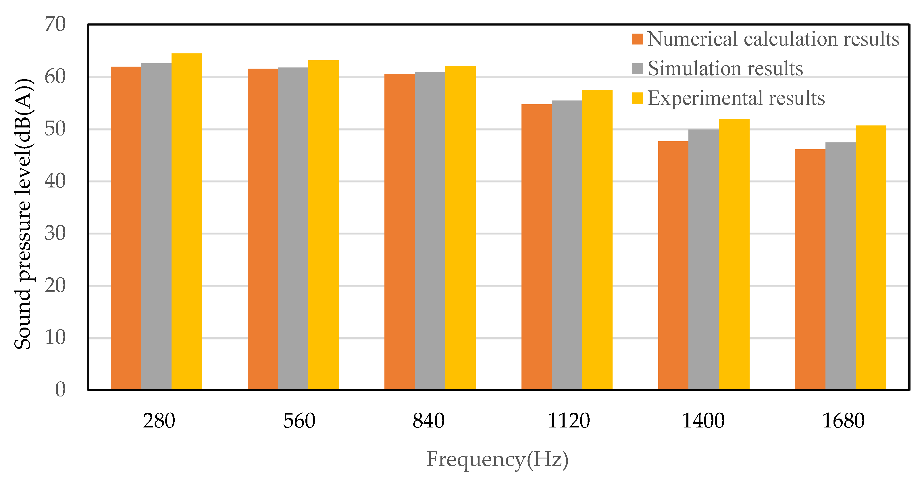
4.2.3. Noise Simulation and Experimental Verification

According to the time–domain calculation results in Figure 5 and Figure 12, the effective value (expressed in dB) within the stable period (at least one period) is obtained using Equation (37). Then, the total sound pressure levels of the fan simulation and experiment are 71.8 dB(A) and 73.3 dB(A), respectively, by weighting A, as shown in Table 3. In order to verify the accuracy of the model, the results of the numerical calculation are compared with those of the simulation and experiment, and the total sound pressure level of the numerical calculation is 0.5 dB(A) less than that of the simulation and 2 dB(A) less than that of the experiment.
The noise spectrum results can be obtained using an FFT transformation of the fan simulation and experimental noise time–domain calculation results that are compared with the numerical calculation results, as shown in Figure 13. It can be seen in Figure 13 that there is a small difference between the peak values of the numerical calculation results, simulation results, and experimental results in the middle- and low-frequency bands. Because the attenuation characteristics of high-frequency noise caused by damping in the transmission process are not considered in the numerical calculation, their results of a high frequency are obviously higher than those of the simulation and experiment.
In order to further compare the differences between the numerical calculation results of the discrete noise and the simulation and experimental results, the first six orders of pulsating noise of the fan are extracted in this paper from Figure 13 (harmonic frequencies are 280 Hz, 560 Hz, 840 Hz, 1120 Hz, 1400 Hz, and 1680 Hz, respectively) for comparative analysis, as shown in Figure 14. The maximum differences between the first and third order pulsating noises through the numerical calculation and the simulation and experimental results are 0.6 dB(A) and 2.5 dB(A), respectively. The maximum differences between the fourth and sixth order pulsating noises through the numerical calculation and the simulation and experimental results are 2.2 dB(A) and 4.5 dB(A), respectively. The above comparison results do not exceed the error target requirement of 5 dB(A) of the spectrum peak, which indicates that the theoretical calculation model is reliable and the error is mainly caused by the simplification of the theoretical model to a certain extent, the inherent errors of the simulation analysis method, and the measurement errors in the experimental process.
It can be seen from the above comparison results that the accuracy of the mathematical model of fan noise obtained from the load force using the new method proposed in this paper meets the requirements, which can be used as an important reference for the study of a high-precision noise mathematical model of low Mach-number fan and blade parameter optimizations.

5. Conclusions

In order to study the influence of the blade parameters of an automotive axial flow fan on its noise and then control the noise of the fan, a new method is presented to obtain the load force and then a mathematical model of the noise and blade parameters of the axial fan of the vehicle is established. The specific research conclusions are as follows: (1) According to the LS blade type, the lift and resistance coefficient curves of the axial fan blade of the vehicle are established, based on this, the constant load force of the blade surface is obtained using the BEM theory and the structural characteristics of the blade of the axial fan. Based on the theory of unsteady thin wings and experimental data, the non-constant load force on the blade surface is obtained, and the constant load force and the non-constant load force are vectors superimposed to obtain the total load force on the blade surface, which provides an important theoretical basis for the study of a high-accuracy noise mathematical model of a low Mach-number fan. (2) Based on the total load force on the surface of the blade and the FW-H equation, a mathematical model of the relationship between the noise of the axial flow fan and the radius, speed, and installation angle of each section of the blade, chord length, and circumferential bending angle is established. The results show that the differences between the total sound pressure levels calculated using the proposed model and the results of the FLUENT software simulation and experimental results are 0.5 dB(A) and 2 dB(A), respectively. The differences between the first and third order pulsating noises using the numerical calculation and the simulation and experimental results are 0.6 dB(A) and 2.5 dB(A), respectively. The maximum differences between the pulsating noises of the fourth and sixth orders using the numerical calculations and the simulation and experimental results are 2.2 dB(A) and 4.5 dB(A), respectively. The above comparison results all meet the accuracy requirements of the model, indicating that the model is reliable, which can provide a theoretical basis for noise control and blade parameter optimizations of vehicle axial fans.

Author Contributions

Conceptualization, Y.Z.; methodology, Y.Z. and Y.L.; software and validation, Y.Z. and J.L.; formal analysis, Y.Z. and Y.L.; writing—review and editing, Y.Z. and Y.L.; supervision and samples made, Y.Z. and J.L. All authors have read and agreed to the published version of the manuscript.

Funding

This research received no external funding.

Institutional Review Board Statement

Not applicable.

Informed Consent Statement

Not applicable.

Data Availability Statement

Not applicable.

Acknowledgments

In this section, Yao Luo (from Dongfeng xiaokang Automobile Co., Ltd.) is acknowledged for his contribution of the experimental equipment.

Conflicts of Interest

There is no conflict of interests in connection with the paper submitted.

References

  1. Available online: https://repairpal.com/radiator-fan-assembly (accessed on 6 June 2020).
  2. Abbas, A.; Elwali, W.; Haider, S.; Dsouza, S.; Sanderson, M.; Segan, Y. CAE Cooling Module Noise and Vibration Prediction Methodology and Challenges; SAE Technical Paper; SAE: New York, NY, USA, 2020. [Google Scholar] [CrossRef]
  3. Mo, J.O.; Choi, J.H. Numerical Investigation of Unsteady Flow and Aerodynamic Noise Characteristics of an Automotive Axial Cooling Fan. Appl. Sci. 2020, 6, 5432. [Google Scholar]
  4. Brooks, T.; Pope, D.; Marcolini, M. Airfoil Self-Noise and Prediction; Technical Report; NASA Reference Publication: Hampton, VA, USA, 1989; p. 1218. Available online: https://ntrs.nasa.gov/search.jsp?R=19890016302 (accessed on 6 June 2020).
  5. Park, S.M.; Ryu, S.Y.; Cheong, C.; Kim, J.W.; Park, B.I.; Ahn, Y.C.; Oh, S.K. Optimization of the orifice shape of cooling fan units for high flow rate and low-level noise in outdoor air conditioning units. Appl. Sci. 2019, 9, 5207. [Google Scholar] [CrossRef] [Green Version]
  6. Zhang, Q. Aeroacoustics Fundamentals; National Defense Industry Press: Beijing, China, 2012. [Google Scholar]
  7. Sun, Y.; Xiao, S.; Xu, X.; Fan, S. Analysis of Aerodynamic Noise Induced by Rotating Blades of an Axial Fan. Noise Vib. Control 2016, 36, 124–128. [Google Scholar]
  8. Zuo, S.; Hu, Q.; Han, H.; Kang, Q. Influence of blade thickness on regenerative blower’s blade noise. J. Vib. Shock. 2014, 33, 130–133. [Google Scholar]
  9. Zhong, Y.; Li, Y.; Li, P.; Chen, J.; Xia, T.; Kuang, X. Blade Structure Design Based on Multi-objective Optimization of Automotive Fan. In Proceedings of the Asia-Pacific Conference on Image Processing, Electronics and Computers, Dalian, China, 14–16 April 2021; Beijing Institute of Physics: Beijing, China, 2021. [Google Scholar]
  10. Zeng, M.; Zhu, W.; Sun, Z.; Zheng, D.; Li, S. Influence parameters of wind turbine blade aerodynamic noise. Appl. Acoust. 2020, 39, 924–931. [Google Scholar]
  11. Zheng, B. Optimization Design of Axial Flow Cooling Fan for Vehicle. Master’s Thesis, Chongqing University, Chongqing, China, 2018. [Google Scholar]
  12. Qian, Z. Prediction of the Noise for the Wind Turbine Rotating Blade Based on FW-H Equation. Master’s Thesis, Nanjing University of Aeronautics and Astronautics, Nanjing, China, 2013. [Google Scholar]
  13. Liu, G.; Wang, L.; Liu, X. Numerical Study on Aerodynamic Performance and Noise Characteristics of Axial Flow Fan with Tip Vane. J. Xi’an Jiaotong Univ. 2020, 54, 105–112. [Google Scholar]
  14. Tian, J. Study on Complicate Flow and Aerodynamic Noise of Axial Flow Fan System in Outdoor Units of Room Air Conditioners. Ph.D. Thesis, Shanghai Jiao Tong University, Shanghai, China, 2009. [Google Scholar]
  15. Oerlemans, S. Wind Turbine Noise: Primary Noise Sources; Technical Report; National Aerospace Laboratory NLR (Royal Netherlands Aerospace Centre): Amsterdam, The Netherlands, 2011; Available online: https://reports.nlr.nl/xmlui/bitstream/handle/10921/117/TP-2011-066.pdf (accessed on 6 June 2020).
  16. Wang, H. Fluid Mechanics; National Defense Industry Press: Beijing, China, 2014. [Google Scholar]
  17. Goldstein, M.E.; Yan, Z. Aeroacoustics; National Defense Industry Press: Beijing, China, 2014. [Google Scholar]
  18. Debertshäuser, H.; Shen, W.Z.; Zhu, W.J. Aeroacoustic calculations of a full scale Nordtank 500 kW wind turbine. J. Phys. Conf. Ser. 2016, 753, 022032. [Google Scholar] [CrossRef]
  19. Rynell, A.; Chevalier, M.; Åbom, M.; Efraimsson, G. A numerical study of noise characteristics originating from a shrouded subsonic automotive fan. Appl. Sci. 2018, 140, 110–121. [Google Scholar] [CrossRef]
  20. Zhong, Y.; Li, Y.; Gao, F. Study on the discrete noise and blade distribution characteristics of a vehicle axial fan. China Mech. Eng. 2019, 30, 1072–1080. [Google Scholar]
  21. Franzke, R.; Sebben, S.; Bark, T.; Willeson, E.; Broniewicz, A. Evaluation of the multiple reference frame approach for the modelling of an axial cooling fan. Energies 2019, 12, 2934. [Google Scholar] [CrossRef] [Green Version]
  22. Hu, X.; Guo, P.; Wang, Z.; Wang, J.; Wang, M.; Zhu, J.; Wu, D. Calculation of external vehicle aerodynamic noise based on les subgrid model. Energies 2020, 13, 1822. [Google Scholar] [CrossRef]
Figure 1. Force of fan blade element.
Applsci 12 07326 g001
Figure 2. Inclined parabolic loading force distribution.
Applsci 12 07326 g002
Figure 3. Calculation flow chart.
Applsci 12 07326 g003
Figure 4. Blade surface loading force distribution along the blade radius.
Applsci 12 07326 g004
Figure 5. Calculation results of fan noise in the time domain.
Applsci 12 07326 g005
Figure 6. Calculation results of fan noise in the frequency domain.
Applsci 12 07326 g006
Figure 7. Fan 3D model.
Applsci 12 07326 g007
Figure 8. The mesh sketch of computing region distribution.
Applsci 12 07326 g008
Figure 9. The graph of sound pressure varying with time at receiving points.
Applsci 12 07326 g009
Figure 10. Sound sensitivity analysis of different mesh sizes.
Applsci 12 07326 g010
Figure 11. Test of single fan’s noise.
Applsci 12 07326 g011
Figure 12. Experimental results of fan noise in the time domain.
Applsci 12 07326 g012
Figure 13. Single fan noise comparison of numerical calculation, simulation, and test results.
Applsci 12 07326 g013
Figure 14. Numerical calculation comparison of single fan discrete noise with simulation and experimental results.
Applsci 12 07326 g014
Table 1. Blade structural parameters.
SectionsRadius/mInstallation Angle°Chord Length/m
Section 10.08800035.00.0544
Section 2 0.09770832.80.0568
Section 3 0.10741730.70.0589
Section 4 0.11712528.70.061
Section 5 0.12683326.90.0631
Section 6 0.13654225.10.0652
Section 7 0.14625023.60.0674
Section 8 0.15595822.20.0699
Section 9 0.16566721.10.0721
Section 10 0.17537520.00.0746
Section 110.18508319.20.0775
Section 120.19479218.60.0806
Section 13 0.20450018.00.0728
Table 2. Circumferential bending angles of different radii.
Radii/m0.08180.1124750.143150.2045
Bending angles/0−4012
Table 3. Comparison of numerical calculation, simulation, and experimental results.
Unit of NoiseNumerical Calculation ValueSimulation ValueExperimental Value
dB(A)71.371.873.3
Publisher’s Note: MDPI stays neutral with regard to jurisdictional claims in published maps and institutional affiliations.

