1. Introduction
To meet people’s pursuit of high-quality life, the household industry is undergoing unprecedented changes. The smart home, with the Internet of Things (IoT) as the core technology, has become the pillar [
1]. Taking the residence as a platform, a smart home organically combines home appliance control, environmental monitoring, information management, audio–visual entertainment, and other functions. Many smart appliances, such as smart lights, smart curtains, and smart door locks, have been widely used and provide a more portable, comfortable, and safe family living environment. To manage the home appliances intelligently and automatically, a centralized automatic control system is used to remotely manage these smart devices, which can be seen as IoT distributed sensor nodes. We can use mobile devices or computers to control them conveniently with local area network (LAN) servers [
2]. Therefore, remote control is the future trend for smart home systems [
3], and communication technology is the key to building a home automatic control system. Earlier systems are mainly based on telephone lines [
4] to achieve remote control. Refs. [
5,
6] introduced phone-based controllers of home and office automation. Later, internet-based remote control solutions for home automation were proposed. Ref. [
7] introduced a wireless solution where the nodes can realize data transmission and interaction with the central server through the wireless communication network. In households, wireless transmission is favored for its flexibility, scalability, and low cost. However, wireless communication systems send data randomly, and the receivers do not know exactly when a data packet arrives. Therefore, how to effectively capture the wireless signals is a fundamental and challenging problem for wireless systems.
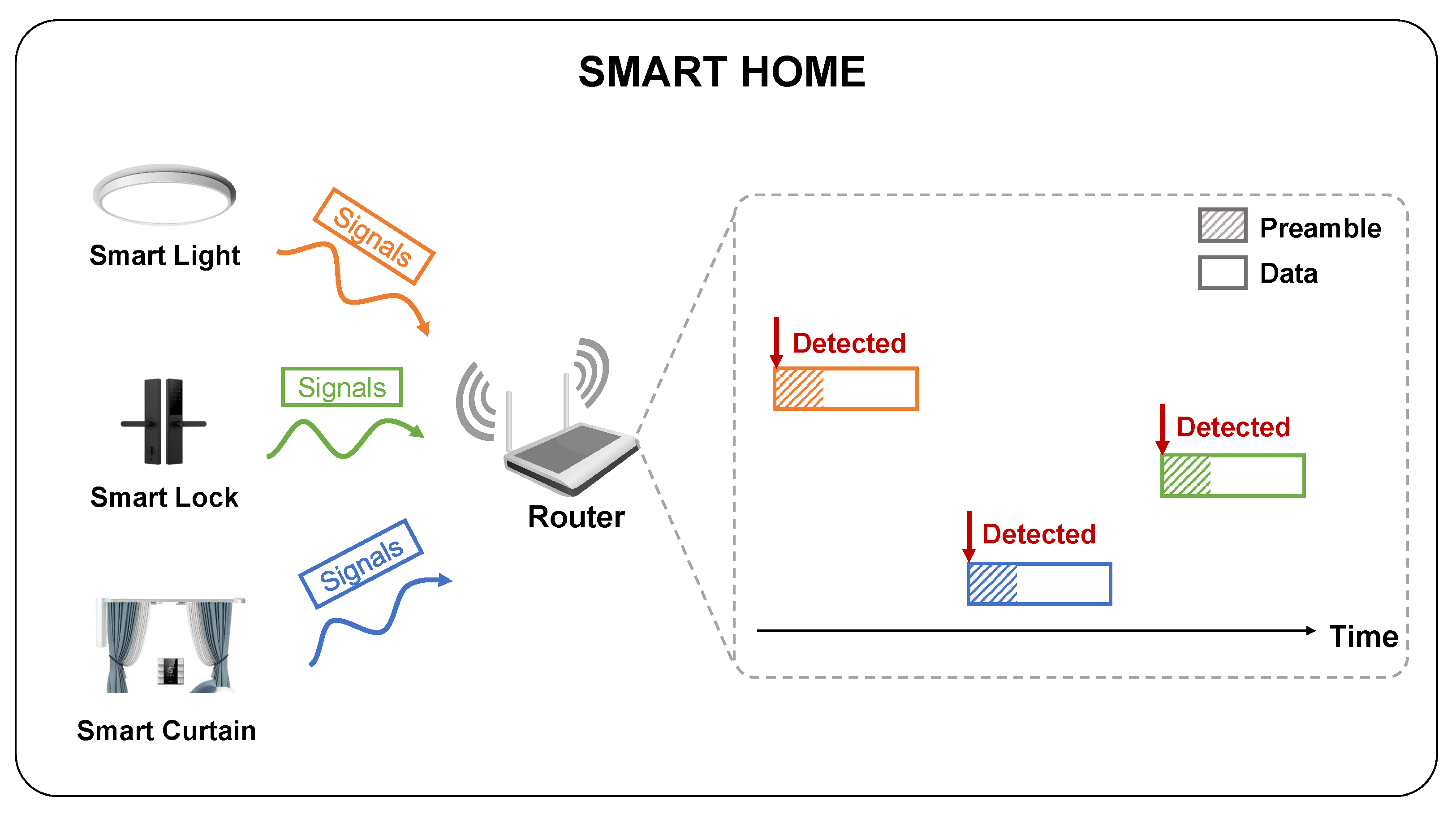
Wireless devices listen for ambient signals continuously to capture data packets timely and accurately. Packet detection determines whether a packet arrives, and is the first and critical step for wireless data processing, as shown in
Figure 1. The remaining operations occur only when a packet is detected. In households, the performance of packet detection greatly affects the communication quality between various smart home devices.
At present, wireless communication systems are mainly divided into two categories, active transmission and passive transmission. The computational complexity afforded by the two systems is diverse due to different system power constraints. The active systems can perform complex operations but require more energy. To obtain enough energy, two main power supply methods, plug-in and battery-based, are used. The former is inconvenient in households and the latter is limited by short lifespan and poor sustainability, and requires regular battery replacement. In recent years, passive wireless communication systems [
8,
9,
10] have become the focus of research. Such systems have an autonomous energy-harvesting module and can achieve near-zero power consumption. They remove the limitation of the battery and make the household wireless sensors able to be deployed once for long-term use, but they cannot perform complex computations due to power constraints. Both systems require packet detection, so when designing detection algorithms, there are two main issues that need to be considered.
Detection accuracy. The detection accuracy is reflected in two aspects. First, the packet detection algorithms should detect packets as correctly as possible, achieving a high detection rate. Second, the start position of the incoming data packet should be found as precisely as possible for better synchronization.
Computational complexity. To meet the requirements of low power consumption for passive wireless communication systems, the computational complexity of the packet detection algorithms applied to such systems must be low. Complex computation should be avoided.
Wireless communication protocols include WiFi, Bluetooth, LoRa, ZigBee, RFID, etc. In households, the most commonly used protocol is WiFi, which has a high transmission rate, long communication distance, and good penetration. Among the protocol standards of WiFi, IEEE 802.11 is the most widely used in daily life. Orthogonal frequency division multiplexing (OFDM) has become the key transmission technique for high-speed mobile communication systems. Therefore, we focus on packet detection algorithms for 802.11 OFDM signals in this paper. Many packet detection algorithms have been applied to existing systems. However, the previous researchers either introduced the algorithms briefly, or just gave an improvement or application of an algorithm. No one, yet, has systematically analyzed and compared these algorithms. Packet detection is a key technical that needs to be broken through, but no major breakthrough has been achieved so far. Therefore, it is necessary to study these algorithms in depth. We delve into the packet detection algorithms and the main work is as follows:
We describe four packet detection algorithms in detail and verify the principle of the algorithms through simulation experiments.
We identify two important factors that affect the accuracy of packet detection and propose methods for algorithm improvement.
We compare the performance of the four algorithms from three dimensions, analyze the characteristics of different algorithms, and point out the applicable scenarios.
We summarize the open challenges and future direction of data packet detection research and introduce several new algorithms that are being studied but have not been widely used yet.
2. Primer Knowledge
2.1. WiFi Receiver Processing
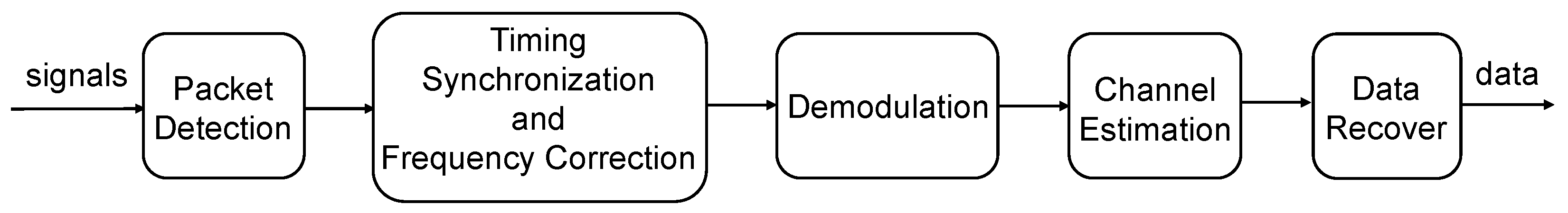
The data processing process on the WiFi receiver is shown in
Figure 2. Packet detection detects the arrival of the signals. Timing synchronization and frequency correction correct the detected signals from the time domain and the frequency domain, respectively. Demodulation converts the received analog signal to a digital signal. Channel estimation evaluates the impact of the transmission channel on packets. Finally, the data are recovered from the signals. All these operations work together to ensure that the transmitted data can be decoded correctly. Among them, packet detection is the first and fundamental operation.
2.2. IEEE 802.11 Standard
IEEE 802.11 is a standard for wireless network communication defined by the Institute of Electrical and Electronics Engineers (IEEE). With the development of technology and hardware equipment, IEEE has successively introduced a series of protocols. Each protocol specifies its communication rates, applicable to different frequency bands, modulation modes, etc.
Table 1 lists several typical 802.11 protocols [
11,
12,
13]. Different modulation modes have their own advantages. Direct sequence spread spectrum (DSSS) has a strong anti-interference ability. It uses a high-speed spread-spectrum sequence to expand the spectrum of the signal at the transmitter, and de-expands and restores the original signal at the receiver. Orthogonal frequency division multiplexing (OFDM) realizes the parallel transmission of high-speed serial data through frequency division multiplexing. It can resist multipath fading and achieve high data rate transmission in multipath channels. Among the modulation modes, OFDM is widely used in 802.11 protocols.
2.3. OFDM Signal Preamble
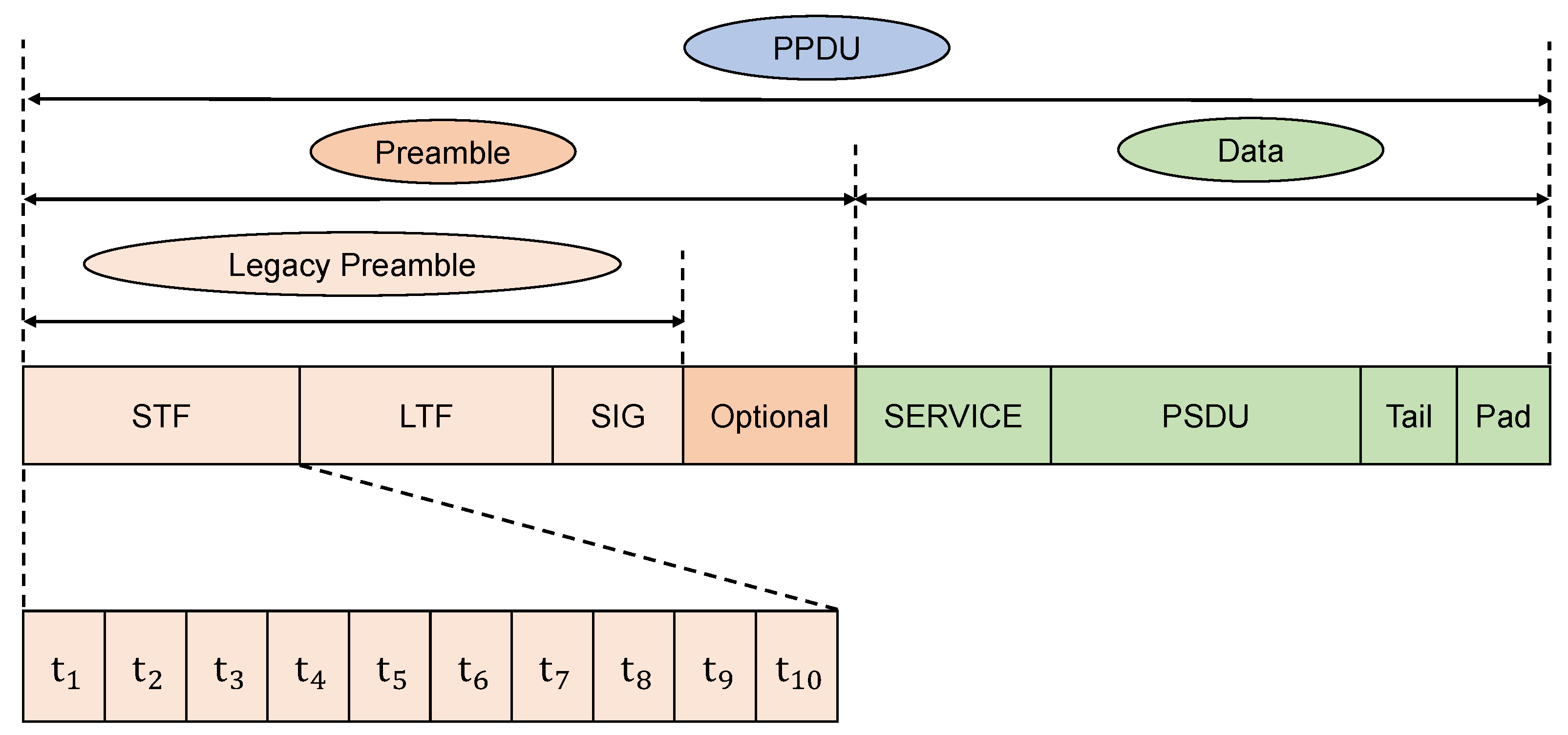
For IEEE 802.11 WLAN OFDM systems, the physical layer protocol data unit (PPDU) is designed for flexible data transmission. PPDU consists of two main parts: preamble and data fields, which are shown in
Figure 3. The preamble field contains the transmission vector format information and the data field mainly contains the payload. Generally, OFDM signals begin with a legacy preamble that is specifically designed for packet detection and synchronization. The legacy preamble contains three parts, which are STF (short training field), LTF (long training field), and SIG (signaling field). STF is used for packet detection and coarse synchronization, LTF is used for fine synchronization and initial channel estimation, and SIG is to determine transmission parameters [
11]. STF consists of 10 identical short symbols, which have good auto-correlation properties. This unique structure is specifically designed by engineers for packet detection and synchronization. STF is simplified as short preamble in the later parts.
3. Packet Detection Algorithms
Generally, packet detection can be described as a binary classification problem [
14,
15]. We regard the detected results as two hypotheses,
and
.
means that the packet is absent and there is only noise.
means that the packet is present.
: Packet is absent.
: Packet is present.
For most detection algorithms, there are two main values, the decision variable and the threshold . When is equal to or greater than , it is considered that a data packet has been detected, and vice versa. Thus, and can also be expressed as follows.
: < ⇒ Packet is absent.
: ≥ ⇒ Packet is present.
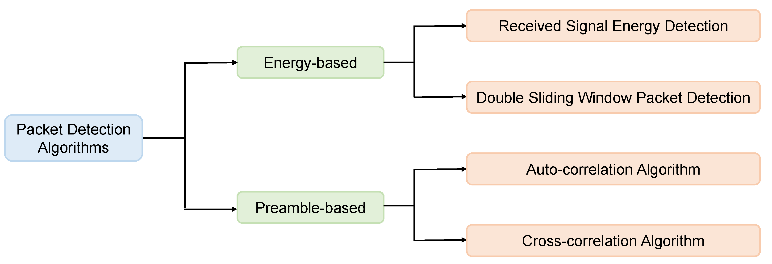
In this section, four packet detection algorithms are introduced, as shown in
Figure 4. They are divided into two categories according to the signal characteristics used: energy-based and preamble-based. The energy-based algorithms use the change of signal energy. The preamble-based ones take advantage of the preamble structure. Simulation experiments were carried out on MATLAB to verify each algorithm’s principle. The experiments were conducted on IEEE 802.11ah with a 10 dB signal-to-noise ratio (SNR). The sampling rate is 20 MHz and the length of one symbol is 16 samples.
3.1. Energy-Based Algorithms
Energy-based algorithms measure the received signal energy and do not require additional knowledge. When there is no packet, the received signal only consists of noise. When the packet starts, the received energy increases due to the signal component. Therefore, there will be an obvious energy change when a signal arrives, and that change can be used for packet detection. The following are two energy-based detection algorithms: received signal energy detection and double sliding window packet detection.
3.1.1. Received Signal Energy Detection
The received signal energy detection algorithm detects packets by directly identifying the change in the received signal energy level [
14], but using only one sample for energy detection is easily affected by single strong noise. A calculation window containing multiple samples is used. The decision variable
is set as the received signal energy accumulated over the window of length
L as Equation (
1). A sliding window can be used to simplify the computation, as shown in
Figure 5. At every time instant n, one new value enters the window and one old value is discarded, so
is calculated by a moving sum of received signal energy by Equation (
2). Therefore, the number of complex multiplications per
is reduced to one received sample.
Simulation. The response of the simulation experiment is shown in
Figure 6. The real start location of the packet is at the index of 101. The sliding window length for accumulation is set as 16 (
L = 16). There is an obvious jump around the index of 101, which is consistent with the real situation. This algorithm is sensitive to noise and is difficult for threshold setting since it directly depends on the received signal energy. The next algorithm reduces reliance on energy power.
3.1.2. Double Sliding Window Packet Detection
The double sliding window packet detection algorithm is also based on received energy, but it uses the ratio of signal power in two consecutive sliding windows to detect packets [
14], as shown in
Figure 7. Two sliding windows,
A and
B, are used to calculate the energy inside them by Equations (
3) and (
4). The lengths of two sliding windows are
M and
L, respectively.
is set as a ratio of the values calculated in two windows by Equation (
5). Thus, when the packet is absent, the response is flat since the two windows contain almost the same amount of noise energy. When the packet comes into window
A, the energy level in
A keeps increasing until
A is totally covered by the packet. Later, window
B starts to collect signal, so
decreases and comes back to flat when
B is covered completely. Therefore,
is large only when the packet is just coming. The sample index n of the peak point in the triangle-shaped response marks the beginning of the packet. The lengths of two windows can be different but can often be set the same for the convenience of threshold setting, which will be discussed in
Section 4.1.1.
Simulation.
Figure 8 depicts the simulated response of this algorithm. The lengths of both windows (
M,
L) are set to 16. There is an obvious triangular peak around the index of 101, which is the real start position of the packet. The other points are very low, which shows that
does not depend on the received power. This algorithm is more noise-resistant than the first one, but has twice the amount of computation. Both the above algorithms need no additional knowledge of packets; however, if the receivers know the packet structure, the following algorithms can be considered.
3.2. Preamble-Based Algorithms
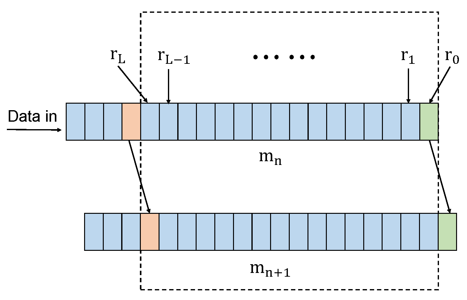
A general communication system engineering principle is that the receiver should use all the available information to its advantage. If the structure of the preamble is known, it should be incorporated into the packet detection algorithms to achieve better detection performance. The following two algorithms, auto-correlation and cross-correlation, use the correlation of the preamble to obtain the decision variable .
3.2.1. Auto-Correlation Algorithm
The auto-correlation algorithm uses the structure of the short preamble and takes advantage of its periodicity [
14,
16,
17,
18,
19,
20,
21]. The 10 repetitive short symbols in the short preamble have good auto-correlation, which are not available in noise and other signals. The algorithm framework is shown in
Figure 9. Although this method also uses two sliding windows, instead of energy calculation, window
C is used to calculate the correlation between the received signal and a delayed version by Equation (
6). When there is only noise, the correlation of noise samples is almost zero since noise does not have auto-correlation characteristics. When the packet is present, the correlation of the identical short preamble is high. The delay
is equal to the period of one symbol length. For IEEE 802.11ah,
D = 16, which is the period of a short training symbol. Window
P is used to calculate the signal energy during the correlation window to normalize
by Equation (
7). The lengths of both windows are
L. Further, both
and
are squared to ensure that
is positive, as shown in Equation (
8).
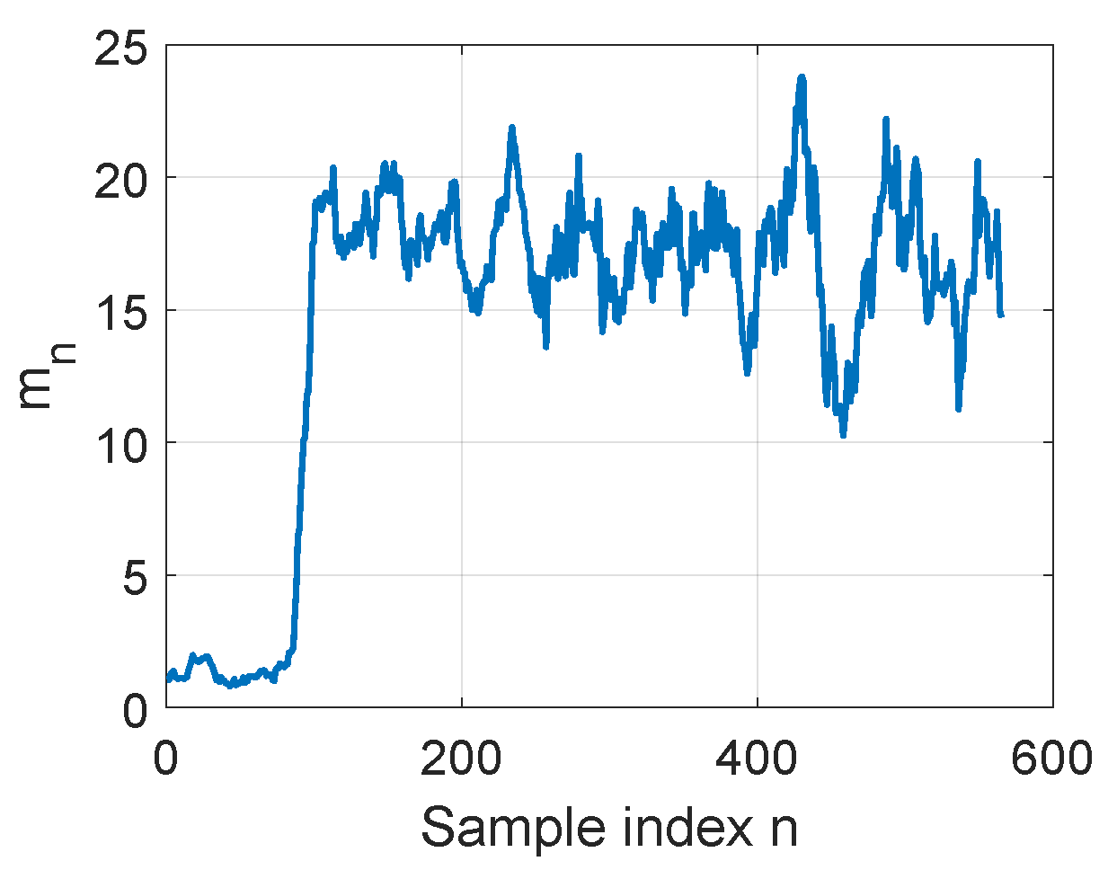
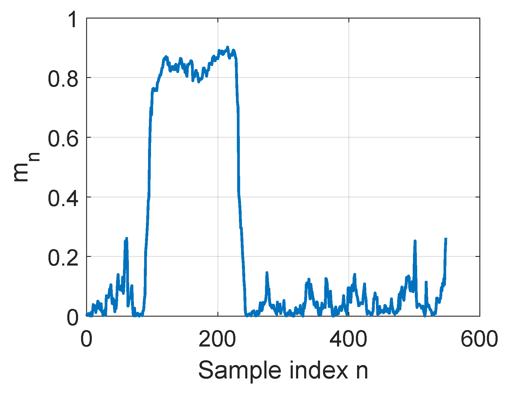
Simulation. The simulation result is shown in
Figure 10. The window size
L is 16.
is high during the whole STF period from index 101 to 260 and remains low before the start of the packet since there is only noise. The difference in response from the double sliding window is caused by the
value. When the packet is present, the correlation result
of the identical short preamble is high, so
jumps to its maximum value. the auto-correlation algorithm only uses the periodicity of the preamble, and there is no need to know the specific content. However, if the structure of the preamble is available, the following method is another good choice.
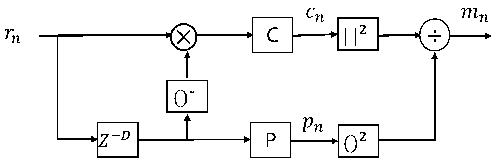
3.2.2. Cross-Correlation Algorithm
The cross-correlation algorithm also uses correlation calculation of the preamble. The difference from the former one is that it uses a template instead of the received signal itself [
15,
17,
22,
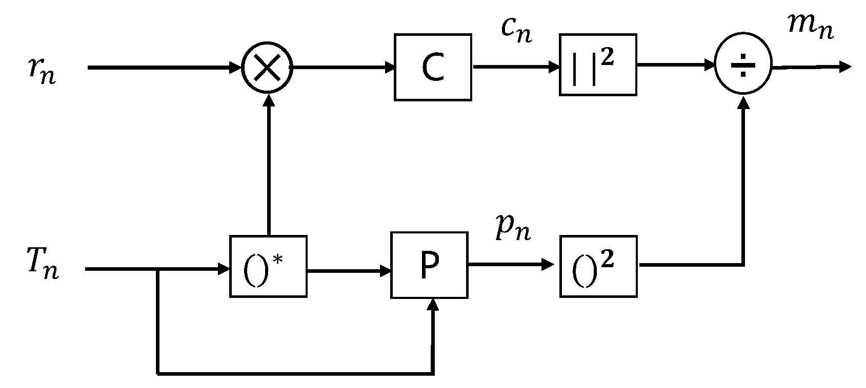
23]. Therefore, completely knowing the preamble structure is the premise of using this algorithm. The flowchart is shown in
Figure 11. In this approach, one symbol from the short preamble is used as a template,
. The cross-correlation is performed between the received signal
and the stored template
. Window
C is used to calculate the correlation between the two signals by Equation (
9). Only when the two parts match is the calculated result large, and the rest of the results small. There will be 10 peaks in the results since STF contains 10 repeated symbols. These peak points are very easy to identify. The correlation result is also normalized by the template signal power calculated in window
P by Equation (
10).
is the same as Equation (
8).
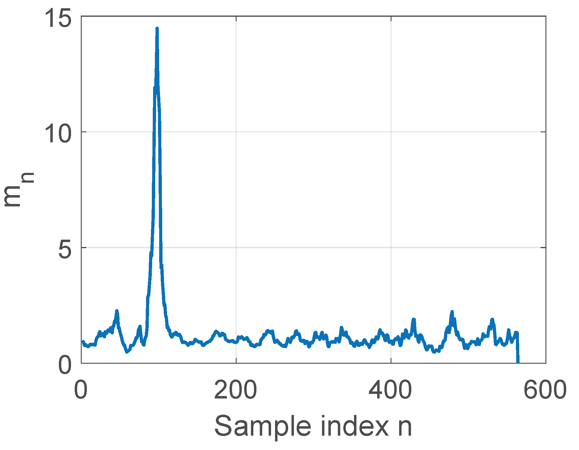
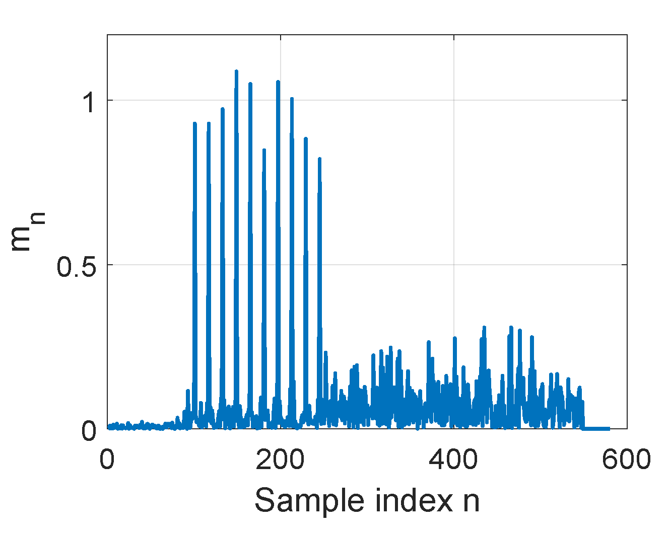
Simulation. The experiment result is depicted in
Figure 12. There are 10 peak points during the index from 101 to 260, which are much higher than others. Especially when there is only ambient noise at the beginning, the matching values are very small. Because the template in this algorithm is fixed, the received signal can only match the template in the specific positions, but for the auto-correlation algorithm, it can be considered that its template is moving along the signal, so
is high during the entire STF period.
4. Analysis and Comparison
In this section, we first give three indicators to judge a detection algorithm, and then analyze how to further improve the detection accuracy. Further, we compare the performance of the above algorithms from three dimensions.
4.1. Measure Metrics
The performance of the packet detection algorithm can be measured by three indicators: the probability of detection
, the probability of false alarm
, and the probability of misdetection
[
24]. False alarm is less severe than misdetection, since missing packets result in data loss. A good algorithm should achieve a high
, which is related to
and
. The algorithm designers must balance them properly. There are two main factors that affect these three indicators: threshold setting and decision rule. The detailed discussions are as follows.
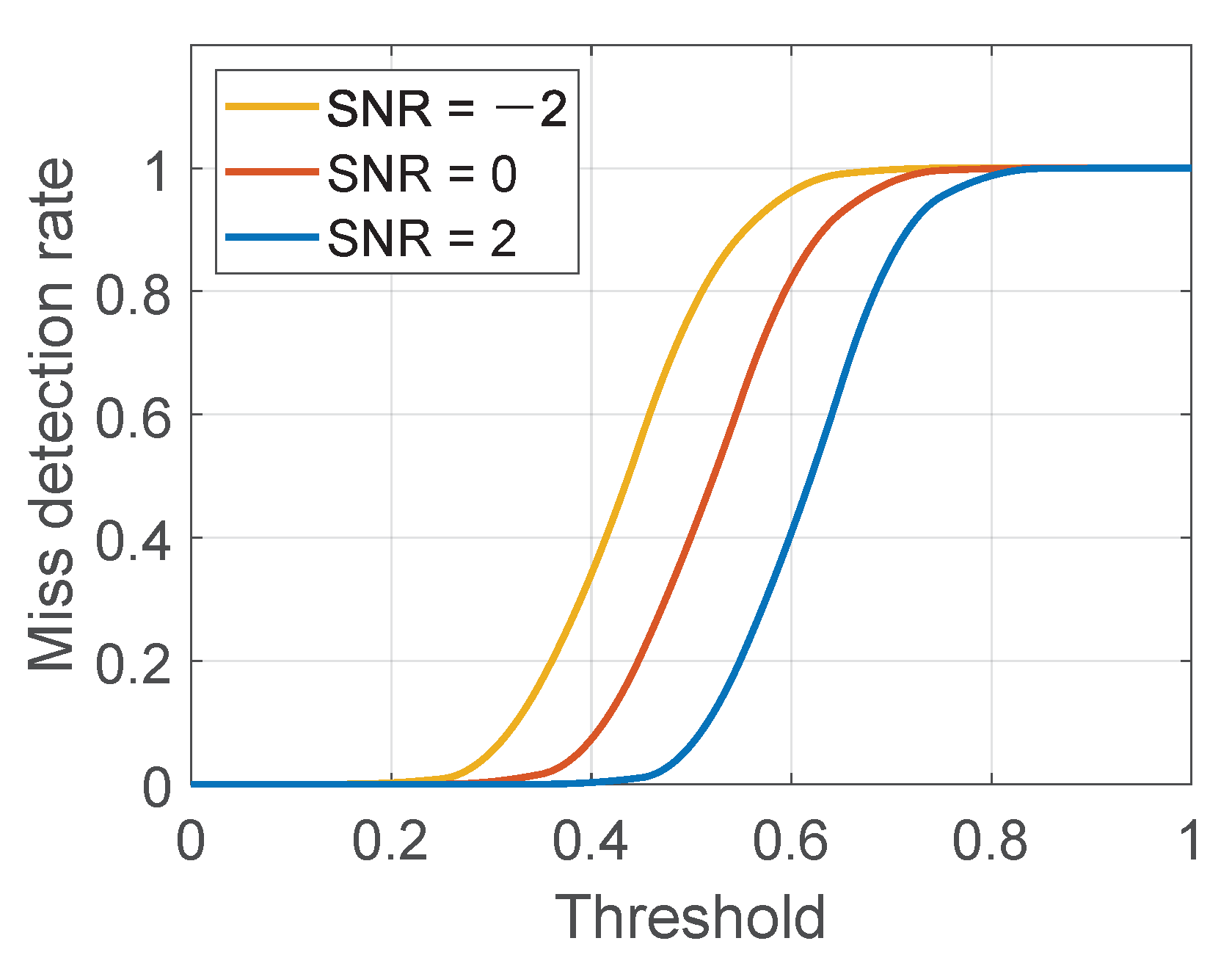
4.1.1. Threshold Setting
When the threshold is too high, most decision variables
are lower than it, so
will be high, and
and
will be low. In contrast, if the threshold is too low,
will also be low since the results may be affected by some larger noise points, which will lead to a high
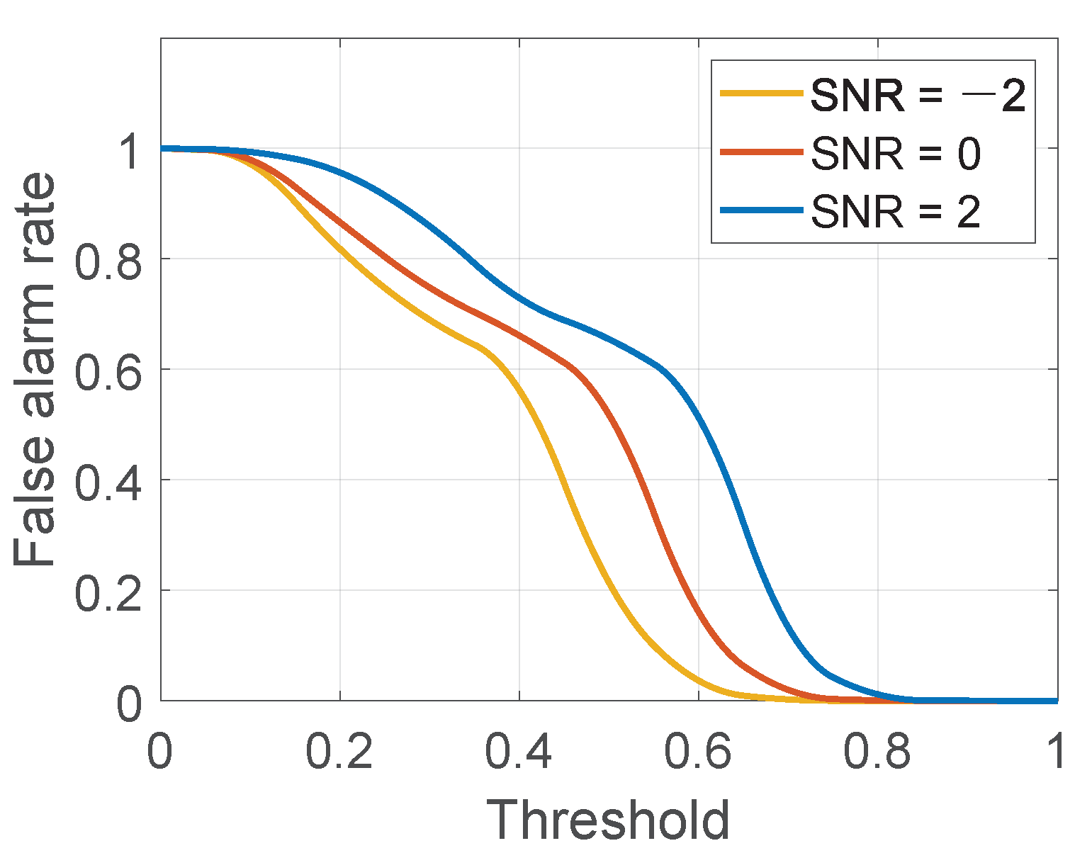
. The changes of
and
with threshold changing are shown in
Figure 13 and
Figure 14 [
25,
26]. The threshold is set from 0 to 1. The simulation experiment uses the auto-correlation algorithm and the SNR is set to −2, 0, and 2, respectively. Overall, as the threshold increases,
decreases and
increases. Due to uncertain environmental factors, it is hard to set a definite threshold, but the setting range of the threshold can be determined. Here are two examples of how to find the range of threshold settings.
Double sliding window. For this algorithm, when the lengths of two windows are the same, the peak point of
can be used as a reference for threshold setting. At
, the value of
contains the sum of signal S and noise N, and the
only contains noise N, thus
can be estimated by the received SNR as Equation (
11). When knowing the SNR in the environment, the threshold setting has a reference range, which is smaller than SNR+1.
Auto-correlation. Similarly, the results of the auto-correlation algorithm can also be denoted by SNR. When the noise signal is additive white Gaussian noise (AWGN), the auto-correlation result of Gaussian noise signal is 0. Thus, there is only the signal power in the numerator after auto-correlation calculation, and the relationship between
and SNR is shown as Equation (
12).
Then, a moderate value in this range is chosen or a fixed scale factor is set, such as 0.75, multiplied by as the threshold. The thresholds for experiments in this paper were chosen properly to balance and , and each algorithm achieves a high .
4.1.2. Decision Rule
Another way to improve is to set up a proper decision rule. The simple method is to compare and . A complex one can be designed based on the characteristics of the response of each algorithm. Here are two examples of decision rule design.
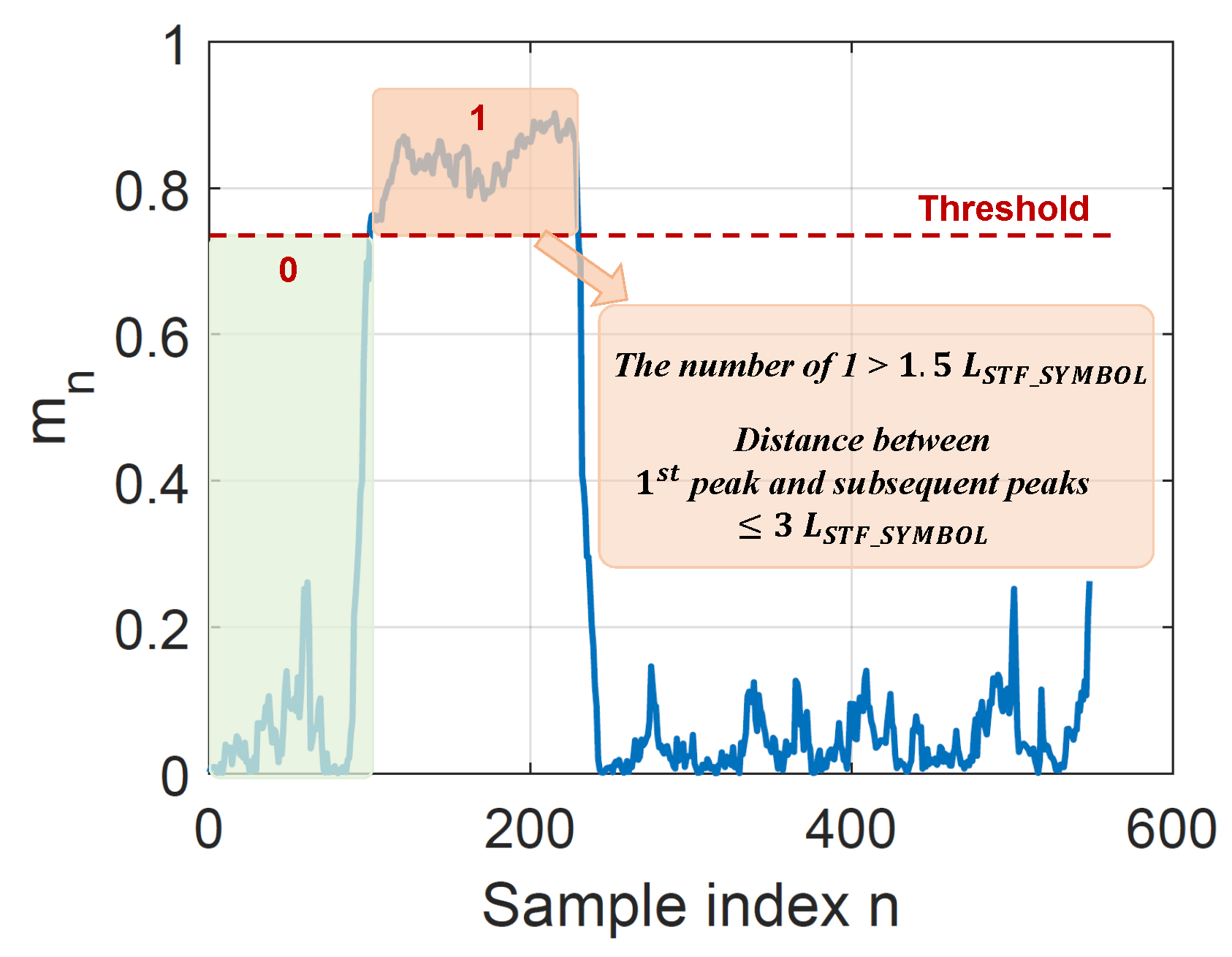
Auto-correlation. According to
Figure 10,
is large throughout the short preamble period. Instead of using only a single point, multiple points can be used together for packet detection. The engineers modified the simple method by setting two judgment conditions in MATLAB sample code. The schematic diagram is shown in
Figure 15. First, it quantifies the
by the threshold.
is set to 1 when it exceeds
; otherwise, it is 0. Then, it is determined whether the number of 1 in the window is greater than 1.5 times the length of a symbol in STF to judge if there are enough points greater than
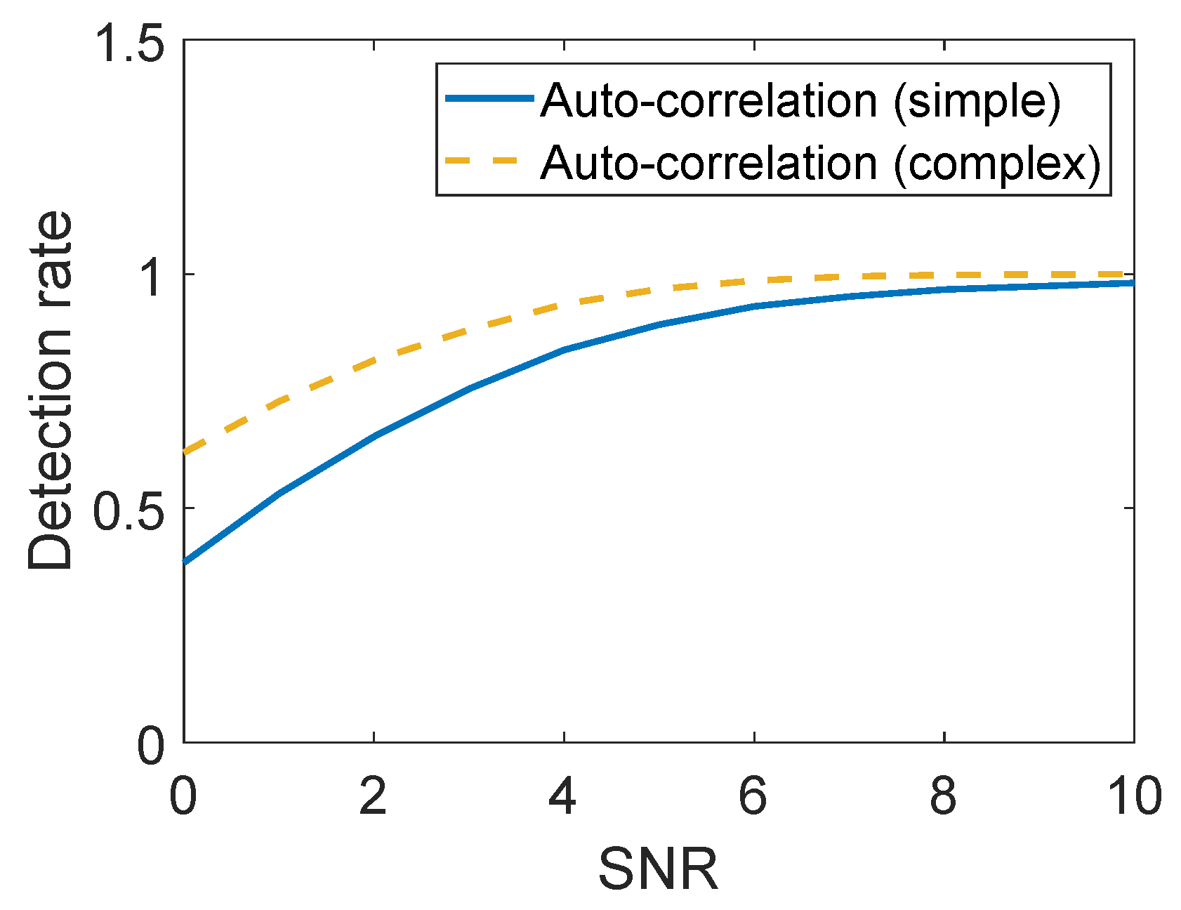
. Second, it is determined whether the distance between the first point and the other points is less than 3 times the length of a symbol in STF. The packet is considered detected only when both conditions are met. The comparison between the simple decision rule and the complex one is shown in
Figure 16. The complex decision rule achieves a higher detection rate because it reduces
well, and the set conditions can be mostly satisfied when the packet arrives, so it will not cause
to increase too much.
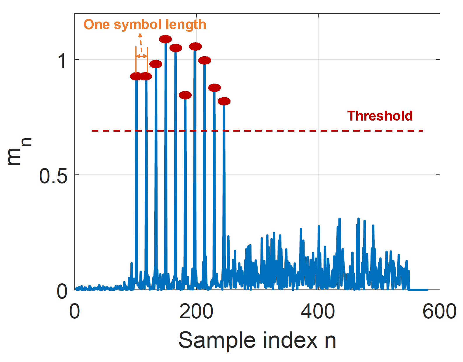
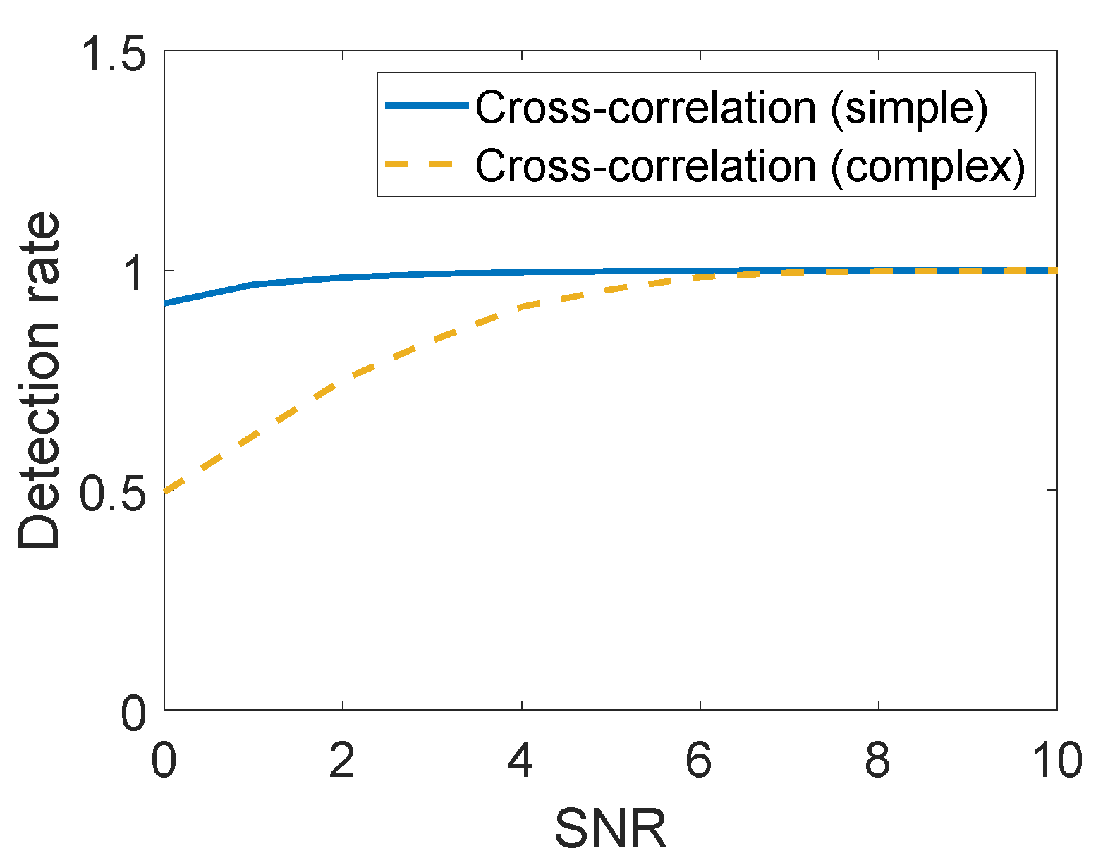
Cross-correlation. According to
Figure 12, there are 10 peak points in the response of the cross-correlation algorithm. Moreover, the distances between these points are equal, which is the length of one short symbol. According to [
15], the authors choose to check all the 10 peaks for detection, as shown in
Figure 17. When the first point exceeds the threshold, they record the index of this point. Then, when the next point is detected, they judge whether the distance between this point and the previous point is exactly the length of a symbol. If checked, they continue to do so until all 10 points are detected. Otherwise, it is considered as no packet.
Figure 18 shows the comparison result, which shows that the simple rule can achieve a better detection rate. It seems to conflict with the previous result. The reason is that the complex approach is too restrictive and results in a high
. Thus, in this case, the simple rule is more suitable than a complex one. Appropriate relaxation of restrictions can have a better performance, which will be studied further in the future work.
Merely comparing the and the is the simplest rule, which may increase because of the large singularity. However, that does not mean that a more complex decision rule is necessarily good, since it will lead to an increase in . Thus, a suitable decision rule is necessary to achieve high .
4.2. Comparison of Algorithms
In this section, we mainly focus on three dimensions for packet detection algorithms: the detection rate, the synchronization accuracy, and computational complexity. To make the comparison reasonable, we use the uniform simple decision rule. The IEEE 802.11ah protocol is used for the simulation experiments. The added noise signal is AGWN and the SNR changes from 0 to 10. To obtain a reliable result, each value is averaged by 10,000 times simulation experiments.
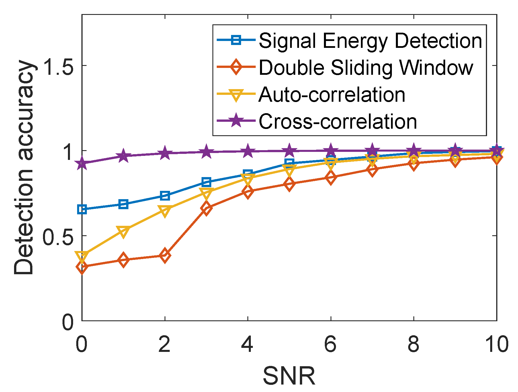
4.2.1. Detection Rate
The most direct criterion for judging the quality of a detection algorithm is the detection rate. To minimize the
, the detected decision is made when the detected position is a half symbol (eight samples for 802.11ah in this paper) around the real position, which is the index of 101 in our experiments. The result is shown in
Figure 19. Overall, the detection rate increases with the increase of SNR. When the SNR is large, the gap between several algorithms is not large, but when the SNR is small, the gap is obvious. Cross-correlation algorithm provides a very high detection rate, which is close to 1. The detection rate of signal energy detection is relatively high. Auto-correlation is centered and the double sliding window detection algorithm is the lowest. The detection rates of the latter two algorithms are below 50% when SNR = 0.
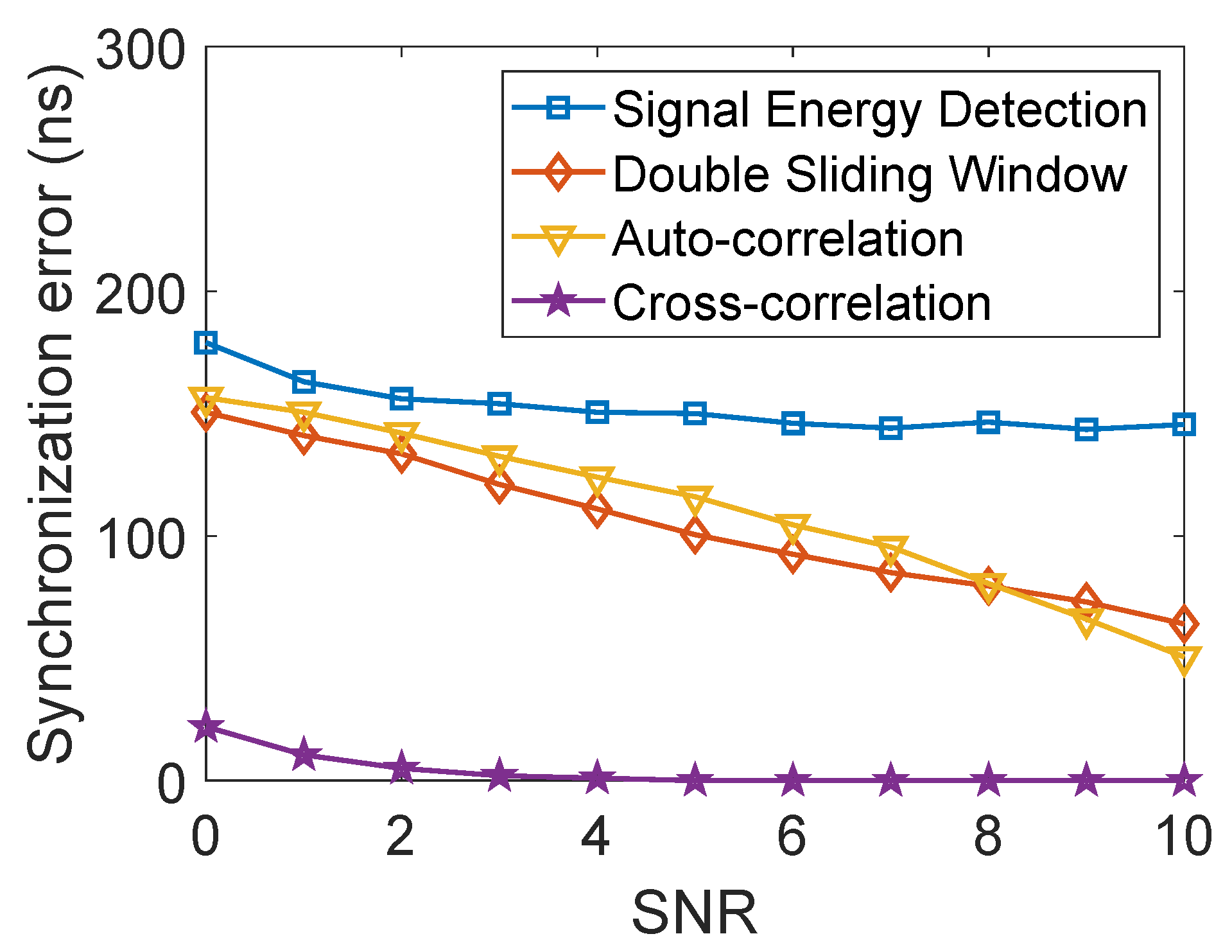
4.2.2. Synchronization Accuracy
After detecting the data packet, it is necessary to find the starting position of the packet, so synchronization accuracy is also important. We use the synchronization error time to measure the accuracy. In the experiments, the real starting position of the packet is at the index of 101. We calculate the average value of the error time between the initial position in the experiment and the real position. The result shown in
Figure 20 indicates that the synchronization error decreases with the increase in SNR. Signal energy detection has the largest error, which is close to 150 ns, and the improvement is not noticeable as SNR increases. Cross-correlation performs much better than others, and has an almost exact detection position. The synchronization errors of the other two algorithms are close and decrease from 150 ns to 50 ns as SNR increases from 0 to 10.
4.2.3. Computational Complexity
Computation complexity is very important when applied to a practical application, especially for low-power hardware. In the experiments, we use the program running time of 10,000 times operations to represent the power consumption. The results are shown in
Table 2. The absolute value is not that important because it depends on the hardware device. We pay more attention to their multiple relationships. The computation complexity of signal energy detection is the lowest. The cross-correlation consumes the most computing resources, which is 3.5× more than the first method. Double sliding window and auto-correlation are about two times larger than the first one.
5. Discussion
Table 3 gives a detailed comparison of the four algorithms. For preamble-based methods, complex decision-rule methods are also included here. The values in the table represent the ranking of algorithms on that dimension.
Signal energy detection is the simplest algorithm, requiring no additional information, and can work on all systems. It has the lowest computational power because it only calculates the energy within a single window. It has a decent detection rate when the threshold is set properly, but it is sensitive to noise and cannot set a fixed threshold since directly depends on the received signal energy. Moreover, the synchronization performance is poor. The reason is that energy accumulation is a continuous process. When the packet arrives, there will be a rising edge for a period of time, and it is difficult to determine the exact start position of the signals.
Double sliding window detection uses the ratio of two windows for detection, so does not depend on the signal energy level and computational complexity is twice that of the former one. Moreover, SNR can be regarded as a reference for threshold setting. In this algorithm, there is an obvious marker point to indicate the starting position of the data packet, so the synchronization error is smaller than the previous one. In theory, the detection rate of this algorithm should be close to or better than the first method, but in experiments, we find that its performance is not as good as expected. Compared with the first one, this method has a certain improvement in synchronization, but it costs twice the power consumption, so it has not been widely used in real systems.
Auto-correlation takes advantage of the 10 repetitive short symbols in the preamble, so it can only be applied to OFDM signals with STF structure. By auto-correlation calculation, the value of is high throughout the STF period. When using a simple decision rule, its performance is similar to energy detection because the above structure is not fully utilized. When the complex rule is used, the performances of detection rate and synchronization are better, but it will bring some increase in computational complexity. Overall, this algorithm has a good trade-off between the three dimensions and is used as an example algorithm for packet detection on MATLAB.
Cross-correlation takes the known short preamble as a template and calculates the correlation between the template and the received signals. will be high only when they are matched exactly. Therefore, a more accurate matching position can be obtained and it can achieve a better synchronization performance. In this case, the decision rules need to be set properly. If the rules are too strict, the detection rate will decrease. The biggest problem with this algorithm is the high computational complexity, especially when the decision rules are complicated. Compared with the previous method, there is no requirement for the structure of the preamble, but the specific content of the signal needs to be known.
All in all, each of these algorithms have their own advantages and are suitable for different scenarios. The auto-correlation has the best overall performance.
6. Open Challenges and Related Work
In this section, we first point out three challenges in package detection and introduce some targeted research work. Then, we introduce the application of the above packet detection algorithms in the actual systems.
6.1. Open Challenges
In a smart home, the above four algorithms can meet the data transmission requirements of active wireless sensors. However, such sensors require battery power and have a limited life. Passive low-power transmission can greatly extend the life of the household wireless sensors but is limited by power consumption. Therefore, the research on packet detection algorithms is still an important subject. At present, there are still three main challenges.
6.1.1. Robust to the Interference
In households, wireless signal transmission faces two problems. First, the room structure is complex, so the signal energy is weakened by many obstructions, such as walls. Moreover, there are many wireless devices, so interference from other devices will affect transmission quality. Some work has been carried out to address this problem. To reduce the SNR of synchronization signals, thereby improving inter-connectivity, Aguilar-Torrentera [
27] uses matched filtering in the form of passive implementation along with cumulant-based processing, which makes this algorithm more insensitive to additive noise. However, this method is only for additive noise. The noise in the actual environment is more complex, so further research is needed.
6.1.2. High Detection Accuracy
The accuracy of data packet detection directly affects whether the household wireless sensors can receive data correctly. The above four are traditional algorithms, they are either simple in calculation but poor in accuracy, or high in accuracy but high in power consumption. Some work modifies these methods to improve accuracy. Yu [
28] improves the energy detection method by two-stage judgment. The first stage roughly detects the valid data. The second stage detects where it has the largest energy near the detection position of the first stage. This method can reduce the false positive rate, thereby increasing the detection accuracy. Others import new technologies to achieve good performance. Ninkovic [
29] introduces a deep learning (DL)-based packet detection algorithm in preamble-based IEEE 802.11 systems. Under some conditions, the performance of the DL-based methods surpasses the conventional methods. However, this method still requires much computing resources. Therefore, how to build a deep learning framework that meets the requirements of low-power wireless sensors is a topic worth exploring in the future.
6.1.3. Low Power Consumption
Low-power transmission technology is the key to extending the life of household wireless sensors. The packet detection algorithms used on such sensors need to reduce the power consumption as much as possible while ensuring the detection rate. She [
30] proposed an adaptive threshold algorithm combining shifting window difference (SWDT) and forward–backward (FBDT) difference in real-time R-wave detection. It can solve the problem of heavily loaded computation caused by the complicated algorithm of the traditional theory. Gong [
31] optimized the cross-correlation algorithm by quantizing the sampled data before performing correlation calculation. Because the raw data are analog signals, which are stored as floating-point numbers, it requires a lot of multiplication to perform correlation calculations. In hardware, multiplication is much more computationally intensive than addition since it requires more D-flip-flops. By contrast, the correlation calculation for quantified data can be achieved by addition. Therefore, they simplify the multiplication operations into addition and reduce system power consumption effectively. However, this method loses some data information and reduces detection accuracy. Therefore, high-accuracy algorithms for low-power systems are worth continuing to explore.
It is difficult to achieve good performance in the above three aspects at the same time. Therefore, for future household wireless sensors, it is very important to take a trade-off on the above characteristics when designing the packet detection algorithms.
6.2. Related Work
The above packet detection algorithms have been widely used in practical systems. In active wireless transmission systems, preamble-based algorithms have better performance. Maier [
18] used the auto-correlation algorithm for wireless access in vehicular environments (WAVE). Adrián-Martínez [
32] used the cross-correlation algorithm for acoustic transient signals in noisy and reverberant environments. That method provides a high SNR, good signal discernment from close echoes, and accurate detection of signal arrival time. Jiang [
33] improved synchronization accuracy and reduced latency through cross-correlation to meet critical industrial control industry needs. In passive wireless communication systems, restricted by power consumption, it is difficult to implement correlation calculation based on preamble. Most backscatter systems, such as [
8,
9,
10,
34,
35,
36], use an energy detection algorithm, which can meet the basic packet detection requirements, but has poor synchronization accuracy. Gong [
31] used a modified cross-correlation algorithm. It achieved a high detection rate and synchronization accuracy, but the performance can be further improved.
7. Conclusions
A household automation system monitors and controls smart home devices remotely using a wireless sensor network (WSN). A WSN consists of a set of sensor technology, computer technology, communication technology, etc. In this paper, we focus on the packet detection, which is a significant step for wireless network communication. We first introduce four packet detection algorithms, which are based on energy power and preamble structure. Then, we analyze the factors that affect the accuracy of the algorithm and provide suggestions for improvement. Further, we conduct a detailed comparison and provide an in-depth discussion of these algorithms from three dimensions. Finally, we analyze the current challenges and future directions in this field. By comparison, we find that the above four algorithms have their own advantages and usage scenarios, among which the auto-correlation algorithm has the best overall performance and is the most commonly used method in existing OFDM systems. Although these algorithms have been widely used in today’s active systems, they have not yet achieved good performance in passive wireless transmission systems. More new algorithms need to be explored and designed to improve the efficiency of packet detection to improve the communication performance of household wireless sensors, and further improve the service quality of the smart home.


