Toward an Efficient Automatic Self-Augmentation Labeling Tool for Intrusion Detection Based on a Semi-Supervised Approach

Abstract

Intrusion detection systems (IDSs) based on machine learning algorithms represent a key component for securing computer networks, where normal and abnormal behaviours of network traffic are automatically learned with no or limited domain experts’ interference. Most of existing IDS approaches rely on labeled predefined classes which require domain experts to efficiently and accurately identify anomalies and threats. However, it is very hard to acquire reliable, up-to-date, and sufficient labeled data for an efficient traffic intrusion detection model. To address such an issue, this paper aims to develop a novel self-automatic labeling intrusion detection approach (called SAL) which utilises only small labeled network traffic data to potentially detect most types of attacks including zero-day attacks. In particular, the proposed SAL approach has three phases including: (i) an ensemble-based decision-making phase to address the limitations of a single classifier by relying on the predictions of multi-classifiers, (ii) a function agreement phase to assign the class label based on an adaptive confidence threshold to unlabeled observations, and (iii) an augmentation labeling phase to maximise the accuracy and the efficiency of the intrusion detection systems in a classifier model and to detect new attacks and anomalies by utilising a hybrid voting-based ensemble learning approach. Experimental results on available network traffic data sets demonstrate that the proposed SAL approach achieves high performance in comparison to two well-known baseline IDSs based on machine learning algorithms.

1. Introduction

With the rapid development of communication, networking has been widely used in all aspects of our daily lives, including power systems, transportation networks, industrial control processes, and critical infrastructures etc. However, in an entrusted communication environment, such systems and their users may be subject to attacks and threats. Thus, in today’s world, network security has become a significant concern for many countries [1,2] to protect their internet-connected systems, including networks, computers, programs, and data from attacks, destruction, or unauthorized access. To do so, many security technologies and approaches have been introduced to cope with emerging threats and the rapid development of attack fashions, including intrusion detection systems (IDSs). IDS is a key component of the cyber security system. It aims to distinguish and identify intrusions from normal ones through computer or network devices by analysing the collected data. In particular, IDS can be classified as a misuse/signature-based approach, where attacks are detected using a database of predefined attack patterns, and an anomaly/behaviour-based approach where normal-operation profiles are built to identify anomalies with respect to behaviours that deviate from the normal ones. The former IDS approach has an advantage of a low false positive rate, but it needs to keep an updated database which is time-consuming and struggles to detect zero-day-attacks. The latter approach has the potential of detecting most types of attacks including zero-day attacks.

In recent years, traffic intrusion detection approaches have been widely introduced and studied as essential tools [1,3] to monitor the normal and anomalous behaviours of network traffic using the machine learning algorithm concept to efficiently and accurately address the issues associated with network attacks, including supervised, unsupervised, and semi-supervised approaches [2,3,4,5]. In general, the supervised approaches are considered as simple, fast, highly accurate, and reliable; however, its main drawback concerns the availability of a predefined label using a large network traffic data set, which is a time-consuming and expensive process. Nevertheless, the presence of noise and incorrect data labeling can certainly reduce the effectiveness of the traffic intrusion detection model [5]. To mitigate the issue of these approaches, unsupervised approaches [3,5] have been investigated and represent a possible means to train anomaly detection models using only unlabeled data which are cheap and easy to collect [3,5]. However, unsupervised approaches do not require domain knowledge experts for the labeling process, and they suffer from low efficiency and poor accuracy [3,5]. Thus, currently, the semi-supervised approaches have been proposed [6,7] to tackle the issues of both supervised and unsupervised ID approaches by combining a small amount of labeled data along with a large set of unlabeled traffic data. However, such semi-supervised approaches suffer from a high false detection rate, especially with the rapid growth of emerging attacks and anomalous. This can be due to the problem of data recall where the network intrusion data set is submerged into a large number of normal traffic flows.

To address the after mentioned issues, this paper proposes a novel automatic self-augmentation labeling approach, namely SAL, which utilises a small labeled data set to efficiently and accurately detect new emerging and anomalous attacks. In particular, the proposed SAL approach has three major phases, including:(i) the utilization of ensemble learning classifiers rather than individual classifiers to overcomes the limitations of a single classifier and accurately predict a class label for a new attack and anomalous, (ii) function agreement to improve the prediction’s ability of the first phase to only label the observations which meet an adaptive confidence threshold, and (iii) an increment update of labeled set phase to iteratively and continuously train a hybrid voting-based ensemble learning approach. In particular, the hybrid voting-based ensemble learning approach, including the soft voting-based and hard voting-based, combines the original labeled data along with new labeled observations which meet the confidence threshold (in phase #2) to assign labels to new coming unlabeled data which may contain new and anomalous attacks.

To evaluate the performance of the proposed the self-augmentation labeling (SAL), two benchmark data sets have been used in the experiment. The experimental results demonstrate the advantages of our proposed approach in terms of accuracy, recall, and F-score measure in comparison to three of the well-known semi-supervised classification algorithms.

The structure of the rest of this paper is organised as follows. Section 2 presents the related work to our proposed approach. Section 3 describes the proposed approach in detail. The performance of SAL in comparison to the other baseline algorithms using two data sets is discussed and summarised in Section 4. Finally, we summarise the research in Section 5.

2. Related Work

We classify existing research into three groups: supervised, unsupervised, and semi-supervised algorithms. For supervised algorithms [3,5,8], the set of all possible traffic flows and output data must be known beforehand. A training data set of sample instances is used to build this classification model. The model that is built can be used to predict the class membership for any unknown instances by analyzing the characteristic values of these flows. Supervised learning mainly helps with organizing new instances into some pre-defined categories by building knowledge structures [3,8]. We aim to provide a set of sample instances which are pre-categorized to the learning machine. The output generated by the learning process is called a classification model. A classification model is built by first examining and then inferring from the set of given inputs. Therefore, the main focus in the supervised algorithm is mapping the input features to the output class and building a model. The knowledge acquired can be manifested as classification rules, or decision trees, or flowcharts, etc. This acquired knowledge is used in the future to classify new instances [5,8]. Supervised learning mainly comprises two levels: training and testing. The first level, called training, is a knowledge-acquiring level which examines the sample data, termed the training data set, and then develops a classification model. The second level, called testing, is used as the classifying step in which the model is created after the training is employed to analyze any unknown instances. Unlike supervised machine learning, clustering techniques do not apply any sample instances for training; alternatively, they create clusters in a given data set applying internalized heuristics.

2.1. Supervised-Based Techniques

This paper [9] introduces a density peaks nearest neighbors(DPNN) classifier based on the core ideas of k-nearest neighbors (KNN) and density peaks clustering (DPC) to improve the accuracy of intrusion detection. Although the results of the experiment indicate that DPNN can perform better than other classifiers in term of average accuracy and efficiency, it cannot detect U2R attacks. Furthermore, in [10], k-nearest neighbor (KNN) [1] has been proven to be efficient in dealing with the feature selection difficulty issues when utilized as its evaluation function. Their proposed algorithm was superior to others in terms of classification accuracy; however, they could also make improvements in the initialization phase. Among the machine learning techniques, researchers have shown that the support vector machine (SVM) can be considered as an efficient algorithm. As an example, Ref. [11] built a robust intrusion detection model with high performance in terms of accuracy, training speed, false alarm rate, and detection rate; however, the authors in this study only worked with the binary case of IDS problems which does not give a realistic model. In addition, a novel intrusion detection technique, named the optimum allocation-based least square support vector machine (OA-LSSVM), was introduced in [12]. This is based on sampling with the least square support vector machine (LS-SVM). Moreover, the experiments in [12] were conducted using KDD 99, which is a standard database considered as the “de facto” benchmark for evaluating performance. The algorithm was suitable for both static and incremental data and obtains a realistic performance. Another research work in [13] presents DoS attacks intelligent detection/defense scheme which improved the detection accuracy to 99.998%, but the main limitation of this algorithm, in addition to the high computational complexity, was that the performance evaluation of the proposed techniques was reported for a typical computer network simulation environment with a sorted dataset, while the effect of the system needs to be tested in the real environment.

Although supervised techniques are usually considered simple, fast, highly accurate, and reliable algorithms, the main drawback is in classifying and labeling Big Data which is expensive or time-consuming due to requiring expert knowledge. On the other hand, noisy or incorrect data labels will certainly reduce the effectiveness of your model [5].

2.2. Unsupervised-Based Techniques

The authors in [14] proposed a hybrid algorithm which is a combination of information gain (IG) and principle component analysis (PCA) for the irrelevant feature of the dataset. They applied multiple ensemble classifiers, which are instance-based learning algorithms (IBKs), multilayer perceptron (MLP), and support vector machine (SVM). In terms of accuracy, time, and detection rates, this novel technique provides good performance. An efficient and secure certificate-less authentication system for VANETs was proposed by [15]. Their system consists of three stages which give privacy to the communications of the group. The registration stage is the first stage, in which a vehicle is registered using a trusted party in the offline mode. The authentication stage is the second stage, in which the vehicle is verified depending on the previous registration stage. The last stage is the shared key between the groups created by the Chinese remainder theorem (CRT). The experimental analysis demonstrates that their design is efficient and can deliver the desired security properties. The researchers in [16] introduced an unsupervised end-to-end deep learning system based on the robust software modeling tool (RSMT) which is considered as an automated monitor and also describes the runtime behavior of the web applications. Empirical analysis was performed through supervised and unsupervised algorithms. The results show that RSMT has produced overhead issues; moreover, tests conducted by applying a supervised ML procedure was poor (at the best case, around 0.728 for XSS using SVM). Furthermore, the unsupervised deep learning achievement was not effective (around 0.906). Although unsupervised-based techniques have emerged as a practical way for learning anomaly detection systems from unlabeled data, and as there is no need for experienced domain experts to label a large amount of data, they suffer from poor accuracy and low efficiency [5].

2.3. Semi-Supervised-Based Techniques

Although most researchers focused on ML algorithms to enhance anomaly detection accuracy, the current researches on semi-supervised techniques are still limited. In [17], a multilevel semi-supervised intrusion detection system was proposed to resolve the non-identical distribution and recall problems using the KDDcup99 dataset. The model shows great improvements in the performance in terms of unknown pattern recognition capability and accuracy; however, the choice of hyper-parameters was not flexible enough and they use a data set to evaluate their MSML framework. Another work in [18] introduced a semi-supervised novel feature-grouping technique based on the linear correlation coefficient combined with the cuttlefish algorithm. They found that it improves the detection rate results and the accuracy rate, though the false-positive rate has significantly reduced. The overall system was tested on KDD cup 99 which is the standard benchmark dataset and, despite the training time being high, it provides good results of high detection rate (95.23%) and accuracy (95.03%) along with a small false-positive rate (1.65%). Here, the authors [19] introduce a hybrid semi-supervised anomaly detection system for high-dimensional data which consisted of an ensemble k-nearest neighbor graph (K-NNG) and a deep autoencoder (DAE). By taking advantage of the strength of the nonlinear mapping algorithm, first, the DAE trained only the essential features of unlabeled data in an unsupervised mode in order to describe a high-dimensional dataset into a more compact data space. Then, a nonparametric of ensemble K-NN classifiers was built from the subsets which was sampled randomly from the specific dataset. The proposed technique was tested using different real-life data sets and the experimental outcomes show that the design enhances the anomaly detection accuracy and also decreases the computational complexity. A semi-supervised anomaly detection system was presented in this paper [20] based on a multivariate statistical network monitoring algorithm, recently proposed, and partial least squares. This solution merged benefits of both supervised and unsupervised approaches. It produces a machine learning system with the same ability to update (zero-day) patterns of malicious activity in a rule-based way. The experiment results of the system based on the real traffic show that the proposed approach can be applied practically. The researchers in [21] recently introduced a semi-supervised detection of outliers (SSDO) which is applied in time series data to monitor water consumption in supermarkets. SSDO holds semi-supervised anomaly detection in two key stages. Firstly, it calculates an anomaly score based on a clustering step. Labels are obtained from the end-user by applying an active-learning strategy. After acquiring labels, the model turns in a semi-supervised mode by utilizing the labels to guide the clustering. The proposed approach was evaluated using several datasets. Empirically, after obtaining a small number of labels, our procedure outperformed the competing procedures compared to unsupervised and state-of-the-art semi-supervised anomaly detection approaches. A semi-supervised procedure was introduced in [22] to detect DDoS attacks, and the unsupervised mode minimizes useless data by using information gain ratio, entropy estimation, and co-clustering, leading to a lower false-positive rate. In the supervised mode, ExtraTrees ensemble classifiers are applied to classify the traffic flows. The proposed algorithm was evaluated using UNSW-NB15, NSL-KDD, and the UNB ISCX 12 datasets, and the best accuracies obtained were 98.23%, 99.88%, and 93.74%, respectively. Despite the algorithm achieving high accuracy, it suffers from complex analysis of unlabeled data and also considers a single classification algorithm.

We conclude that existing semi-supervised-based intrusion detection techniques are a cost-effective option since domain experts are not fully needed to get involved in the process of labeling training data sets. However, these types of techniques suffer from poor accuracy and low efficiency. Motivated by this, we will develop IDS upon exiting solutions by reducing the need for domain experts to classify thousands and thousands of data flows. At the same time, this framework aims to minimize the false positive rate while maximizing accuracy.

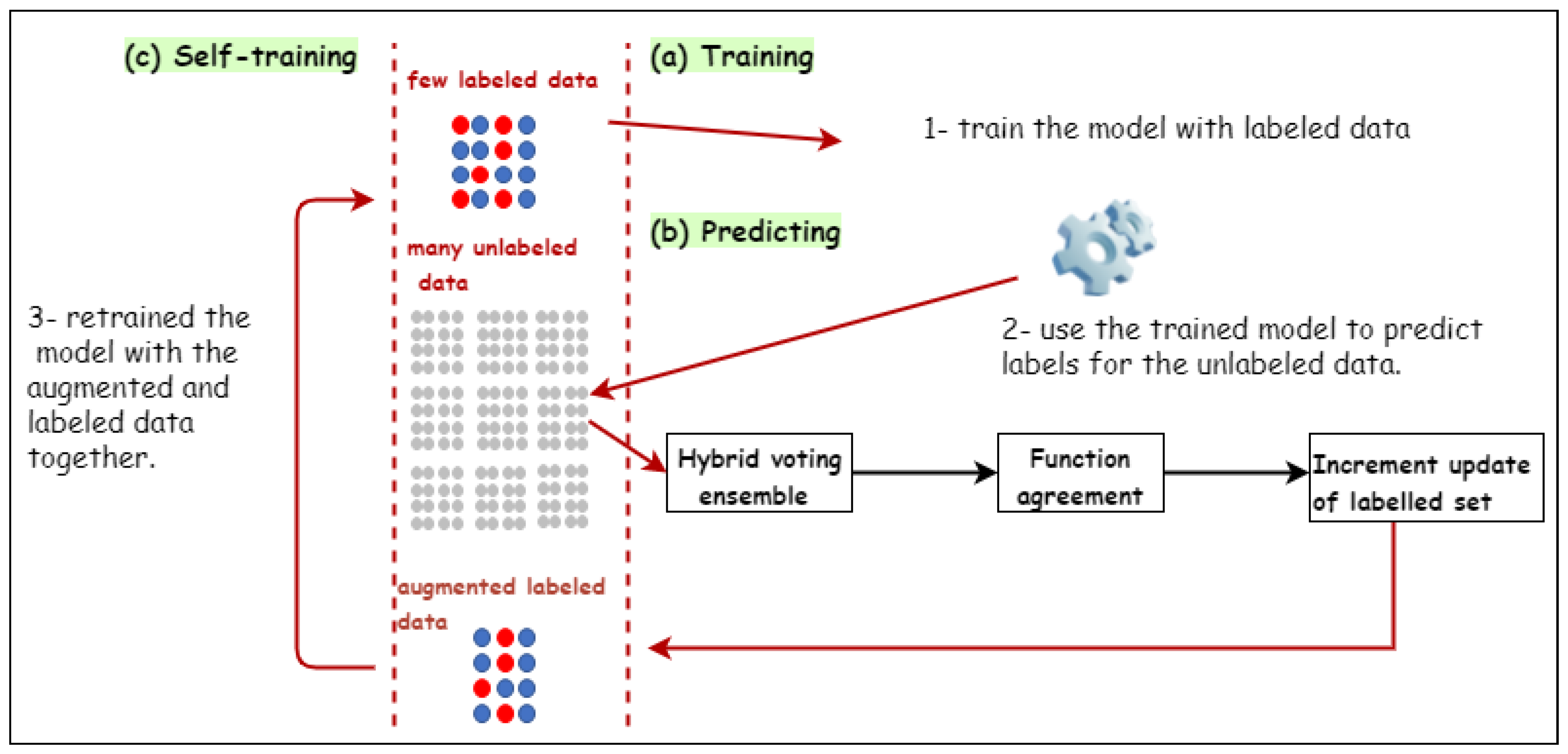
3. SAL: Proposed Self-Augmentation Labeling Approach

With the goal of improving the accuracy of network-based intrusion detection systems (NIDSs) with less domain experts’ involvement in the labeling process, semi-supervised-based techniques have been proposed with the aim of limiting labeling costs [17,18,22]. However, the accuracy of proposed semi-supervised is based on the percentage of the labeled data and how they are representative to each distribution in the original data set. In other words, the higher the availability of labeled data, the better the accuracy results. To address the above concerns, we propose a novel semi-supervised lablling approach that performs automatic labeling, called self-augmentation labeling (SAL), which labels unlabeled observations by utilizing the available labeled and unlabeled observations. Two processes are involved in this operation: labeling and augmentation processes, and they are looped sequentially and executed until all traffic observations are labeled. A general overview of the proposed approach is presented in Figure 1. In particular, the proposed approach begins with labeling the data using a very small data set under very strict constraints in the first iterations in order to obtain correctly labeled data. Then, the labeled data are combined with the original labeled data in order to increase the amount of labeled data for better learning. In the first iterations, the proposed approach focuses on the adequacy, not the quantity, of the labeling process. This is because combing incorrectly labeled data with the original labeled data can result in incorrect learning in the next iteration of labeling. In the labeling process, we use a hybrid voting-based ensemble learning approach, which combines the features of soft voting-based ensemble and hard voting-based ensemble learning approaches, and a set of parameters can be imposed on the learning process in the proposed approach.

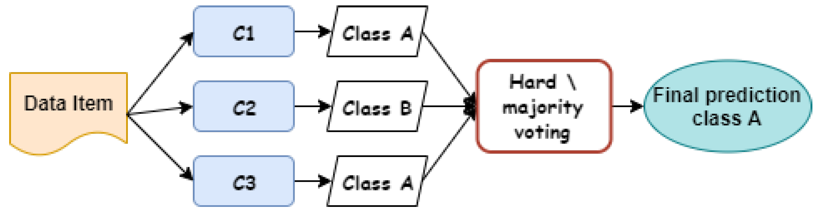
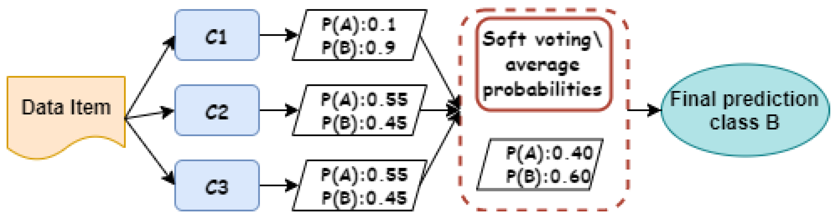
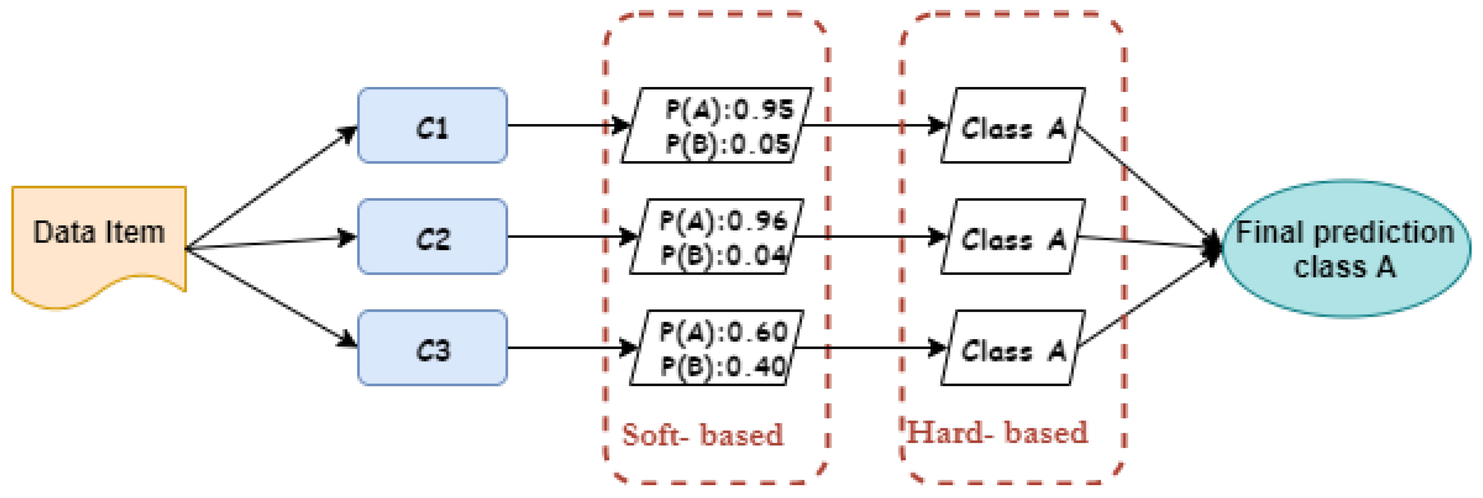
3.1. Hybrid Voting-Based Ensemble Approach

With the goal of producing accurate results that outperform those of any individual classifier, we propose an ensemble of classifier approach to aggregate their predictions and produce a class label for a new data item [23,24]. The voting classifier is one of the popular and powerful ensemble classifiers which takes input as two or more estimators and classifies the data based on majority voting [24,25]. By combining the multiple prediction models, it overcomes the limitations of single base classifiers and outperforms the overall results. Voting classifiers use two voting approaches: (i) majority/hard voting and (ii) soft voting [26]. With the hard voting, each individual classifier has one vote and the class label for a data item is the class with the majority that was predicted by each single classifier, while soft voting is the same as the hard voting in terms of the use of a set of different classifiers to make the final decision of the appropriate class of the data item; however, each individual classifier assigns a probability score for each class and the most probable class is the one that obtains the largest average probability of all the candidate classifiers.

Definition 1.

Let us define the decision of the $cth$ classifier as $d_{c_i,w_j}\in$ {0,1}, i = 1, …, C and j = 1, …, W, where W is the number of classes and C is the number of classifiers. If the $cth$ classifier chooses class $w_j$, then $d_{c_i,w_j}=1$, and 0 otherwise. The final decision of both hard and soft voting can be defined by Equations (1) and (2), respectively.

$$\widehat{y}=\underset{j}{argmax}\sum _{i=1}^C{d}_{c_i,w_j}$$

(1)

$$\widehat{y}=\underset{j}{argmax}\sum _{i=1}^C{P}_{c_i,w_j}$$

(2)

We weighed the predictions of each base classifier equally. In Equation (1), class $w_j$ will be chosen as the final prediction $\widehat{y}$ if its sum of votes from all classifiers $i=1,\dots ,C$ achieve the maximum sum among all classes $j=1,\dots ,W$. While in Equation (2), the final predicted class $\widehat{y}$ will be the class that achieves the highest probability $P_{c_i,w_j}$ among all classes where $P_{c_i,w_j}$ is the probability that is assigned to the ith class with jth classifier.

Figure 2 and Figure 3 show illustrative examples that demonstrate the calculation processes of both hard and soft voting techniques in ensemble learning. In hard voting, as depicted in Figure 2, there are three classifiers whose individual decisions are combined to predict whether the data item is an instance of class A or class B. As we can see, both classifiers $c_1$ and $c_3$ predicted the data item as class A, which is considered as a final decision because it gains the majority of voting. As shown in Figure 3, the ensemble decision making of soft voting is different from hard voting, whereas a probability value is assigned to each class by each classifier. As seen, both classifiers $c_2$ and $c_3$ assigned 55% of the data item belonging to class A. However, both classifiers $c_2$ and $c_3$ assigned high probability scores for the data item that belongs to class A. Class B is the most probable class for the data item because this class obtains the largest average probability value of all classifiers $c_1$, $c_2$, and $c_3$, which is 60%, while the average probability value for the data item belonging to class A is 40%.

Although hard voting is the simplest and most common strategy in ensemble-based decision making, the final decision is based on majority votes irrespective of the total agreement of classification models. Soft voting, on the other hand, incorporates each classifier’s prediction into the final decision through taking average prediction probability scores. In the former, the classifier’s decision that does not consent with the majority of the participating ones will be excluded from the final decision, while in the latter, the classifier will participate in the final decision even with a low prediction probability score. The accuracy performance of both techniques is almost entirely dependent on the amount of labeled data.

Therefore, the percentage of available labeled data is critical because it affects both hard and soft voting techniques’ performance. The more labeled data that are available, the more accurate the results. To tackle the above problem, we aim to optimize the accuracy performance of the labeling processes even with a tiny labeled dataset. This is performed by hybridising hard voting with soft voting to build a robust model that is able to control threshold tuning for a strong labeling process. In addition, the proposed approach imposes additional restricted rules for the labeling process, especially in the first steps, where we have a negligible percentage of labeled data. In the proposed hybrid voting ensemble technique, a soft voting technique is applied to compute prediction probability scores for each unlabeled observation using a number of classifiers. Therefore, if the prediction probability score from all classifiers exceeds the given threshold, then the predicted label is assigned to the unlabeled observation. Due to the small size of the labeled data set, we intend to start with strict constraints to ensure that the unlabeled observations are labeled as accurately as possible. The strict constraints are preserved or relaxed based on the amount of labeled data in each iteration of the labeling process. The final decision in the proposed hybrid ensemble voting approach is presented in the following definition.

Definition 2.

By holding the assumptions in Definition 1, the final predicted class $\overline{Y}$ for each unlabeled observation is $w_j$, if, and only if, the following conditions hold:

$$\sum _{i=1}^C{d}_{c_i,w_j}=C$$

(3)

$$\underset{j=1}{\overset{W}{max}}P\left(w_j\right)>\alpha \forall c_i\in C$$

(4)

where $P\left(w_j\right)$ is the prediction probability score for $w_j$ class and α is the predefined labeling threshold.

As illustrated in Figure 4, three classifiers are used to predict the correct label of a given observation, and the first classifier predicts that the observation belongs to the class A by 95%, while the second classifier predicts that the observation belongs to class A by 96%. With remarkable difference, the third classifier predicts that this observation belongs to the class A by 60%. In this illustration, the final decision for both hard and soft voting techniques is that the given unlabeled observation belongs to class A. This is because the hard voting approach is based on majority, and as we can see, all classifiers agree that this type belongs to A. Likewise, the second soft voting technique will classify this type as class A because the average probability score of this observation belonging to class A is quite high. However, the proposed approach does not treat this observation in this manner; rather, there are constraints that influence the final outcome, which can be controlled by the parameters that will explained in the next section.

3.2. Function Agreement

In machine learning, we deal with two types of parameters: (i) machine learnable parameters and (ii) hyper-parameters [27]. The machine learning parameters are the ones which the algorithms learn/estimate on their own during the training for a given dataset. On the other hand, the hyper-parameters are the ones which the machine learning engineers or data scientists will assign specific values to, in order to control the way the algorithms learn, and also to tune the performance of the mode. Since the labeling process in the first stage is subject to strict constraints to ensure that the data are labeled as accurately as possible, we will define and explain two hyper-parameters that completely control the self-augmentation labeling process in our proposed model as follows:

1

Labeling threshold. This threshold $\alpha$ represents the minimum acceptable probability for labeling the observations. In order to improve the classification accuracy for the results, we will start with a very high value of $\alpha$ to ensure that only the most accurately labeled observations are classified. The value of this threshold can be tolerated (decreased) by a fixed value which is denoted as $\gamma$; this means that the threshold $\alpha$ is decreased by $\gamma$ when the value of learning rate meets the predefined criterion.

2

Learning Rate. The learning rate (LR) is a hyper-parameter that measures the rate or speed at which the model learns the values of the parameters. It evaluates how quickly the model adapts to the problem. In the proposed algorithm, the labeling threshold value is considered the most effective factor on LR. As a result, a high $\alpha$ value leads to a smaller LR, implying that more training is required. On the other hand, as the value of the $\alpha$ threshold is decreased, the LR increases, resulting in faster changes and less training. Let $L_i$ denote a variable that represents the number of labeled observations at iteration i, and $U_i$ is a variable that represents the number of unlabeled observations at iteration i.

Typically, in our model, LR will be calculated for each iteration i as follows:

$$\mathrm{L}{\mathrm{R}}_i=\frac{L_i}{U_i}$$

(5)

Since the proposed approach aims to improve the accuracy as much as possible, which is influenced by the amount of labeled data, we will define the $\beta$ threshold which denotes the maximum value of the learning rate that updates the $\alpha$ threshold to ensure that the $\mathrm{L}\mathrm{R}$ will not be stuck in a constant. So, any $\mathrm{L}\mathrm{R}$ that exceeds this threshold will block the $\alpha$ updating in the iteration. So, the $\mathrm{L}\mathrm{R}$ value, along with $\beta$ and $\gamma$ thresholds, will guide the $\alpha$ threshold decrement process as follows:

$$\mathrm{Decrement}\left(\alpha \right)=\left\{\begin{array}{cc}\alpha =\alpha \hfill & ,\mathrm{If}\mathrm{L}\mathrm{R}>\beta \hfill \\ \alpha =\alpha -\gamma \hfill & ,\mathrm{If}\mathrm{L}\mathrm{R}<\beta \hfill \end{array}\right.$$

(6)

The reason behind decreasing the $\alpha$ threshold is because after some number of iterations, we will be unable to find observations that meet the criteria of a high value of $\alpha$. Figure 5 shows the relation between the number of iterations with and without updating the $\alpha$ threshold and it indicates that without this updating process, after a number of iterations, the $\mathrm{L}\mathrm{R}$ will be a constant function.

3.

Illustrative Example. An example is presented below to explain the proposed model’s labeling process. Given three selected supervised classifiers ($C=C1,C2,C3$) that are trained on a small labeled dataset to provide decision models ($M=M1,M2,M3$), in this example, each unlabeled observation belongs to one of five possible labels as follows: $L1,L2,L3,L4,L5$.

Now, assume that U is the set of unlabeled observations. For a given unlabeled observation $x_u\in U$ and with a given threshold value ($\alpha =0.95$), the labeling process is performed using the following steps:

(1)

The probabilities of $x_u$ are predicted as shown in

Table 1. Prediction results for a single observation $x_u$ using three decision models.

Decision Model	M1	M2	M3
Is observation $x_u\in L1$ ?	0.98	0.99	0.97
Is observation $x_u\in L2$ ?	0.009	0	0.01
Is observation $x_u\in L3$ ?	0.01	0.008	0.01
Is observation $x_u\in L4$ ?	0	0.002	0.005
Is observation $x_u\in L5$ ?	0.001	0	0.005
Sum	1	1	1
Max	0.98	0.99	0.97

.

(2)

The higher probability for each classifier is found and compared with the $\alpha$ value.

(3)

$L1$ is assigned to the observation $x_u$ since all classifiers agree on it.

Then, Equation (4) is used to compute the final prediction $\overline{Y}$ for $M1$, $M2$, and $M3$, respectively.

For M1,

$$(\underset{L1}{\overset{L5}{max}}P\left(x_u\right)=0.98\mathrm{and}0.98>0.95)⟶\overline{Y}=L1$$

(7)

For M2,

$$(\underset{L1}{\overset{L5}{max}}P\left(x_u\right)=0.99\mathrm{and}0.99>0.95)⟶\overline{Y}=L1$$

(8)

For M3,

$$(\underset{L1}{\overset{L5}{max}}P\left(x_u\right)=0.97\mathrm{and}0.97>0.95)⟶\overline{Y}=L1$$

(9)

3.3. An increment Update of Labeled Set

Since our labeling model was trained using a very small labeled dataset, an iterative increment update of labeled observations process will be used to augment new labels for a larger set of unlabeled data; these new labels, along with the originally labeled dataset, are utilized in the next iteration to retrain the model. Such an iterative process will improve the labeling process besides the accuracy of the detection model. Moreover, in order to produce a stronger detection model with as accurate results as possible, this small labeled dataset must be subject to restricted rules, as explained in Section 3.2. The threshold $\alpha$ is continuously decremented when $\mathrm{LR}<\beta$. The labeling process will be repeated until all observations are labeled. Algorithm 1 shows the detailed steps of the SAL algorithm. data structures, variables, and functions applied by the algorithm are summarized in

Table 2. Variables, data structures, and functions employed by Algorithm 1.

Self-Augmentation Labeling Processes Algorithm
L	The labeled subset of the training data.
U	The unlabeled subset of the training data (the most part).
C={C1,C2,C3}	Set of the selected supervised base classifiers used to build the decision model.
$Vens$	The model that trains on an ensemble to predict an output (class) based on the class with the highest probability of being the output.
$\alpha$	Predefined labeling threshold represents the minimum acceptable probability for labeling the observations at each iteration start initially with a very high value.
$\beta$	Predefined amount from the training data set denotes the maximum value of the learning rate which allows the updating of $\alpha$ threshold, so any LR that exceeds this threshold will block the updating at that iteration.
$\gamma$	Threshold step (predefined value) to decrement the $\alpha$ threshold.
$left$	A list represents the number of unlabeled observations in each iteration.
$u_i$	Any single observation belongs to U.
i	Incremental variable starts initially by 0.

.

Algorithm 1 Labeling Process

Input: Labeled data set L;          Unlabeled data set U;          $C=\{C1,C2,C3\}$: base learning algorithms.          $Vens$: voting Ensemble Classifier.

Output: Fully labeled data set

Process:  1: Set 3 Threshold values: ($\alpha ,\beta ,\gamma$ ).  2: $left\leftarrow \Phi$.      ▹ set of left unlabeled data.                                                         3: while (U is ! empty) do  4:       $Vens(L,C)$    ▹ Use L to train ensemble classifier                                             5:       for each $u_i$ in U do    ▹ Initial $i=0$                                                                     6:             $left\left[i\right]\leftarrow Count\left(U\right)$  7:             While $\left(left\right[i-1]-left[i\left]\right)<\beta$ do  8:                   Remove $u_i$ From U  9:                   Add $u_i$ To L  10:             if $\left(left\right[i-1]-left[i\left]\right)>\beta$ then  11:                   $\alpha \leftarrow \alpha -\gamma$      ▹ Updating $\alpha$

4. Experiment Results and Comparison

In this section, we conduct an experimental study to demonstrate the effectiveness of the proposed algorithm on well-known benchmark traffic flow data sets. As an illustration, we compare the proposed SAL approach against two baseline algorithms, including the probabilistic graphical model (PGM) [7] and various widths clustering (kNNVWC) [28]. Section 4.1 describes the network traffic data sets and Section 4.3 presents the evaluation metrics. Third, the experimental settings for a proposed SAL approach and the baseline algorithms and its procedure are specified in Section 4.4. Finally, we present and explain the results and findings of our experiment and compare it to the baseline algorithms in Section 4.5.

4.1. Data Sets Used in Experiment

Data sets gathered from different environments are distinct and this makes it essential to identify the appropriate data sets. These data sets are typically used to meet a variety of classification requirements. The analysis of various data sets allows us to gain a more comprehensive understanding of a traffic classification algorithm. This is due to the fact that researchers usually select different data sets in order to meet their requirements [2]. For example, if the goal of a classification process is to detect various types of network attack traffic, they must select data sets that include a variety of malicious traffic for analysis. The proposed approach is evaluated using two data sets. These data sets have been chosen since they were collected from a variety of domains and are commonly used to evaluate anomaly detection systems. Detailed descriptions of both data sets are explained in the following two sections.

4.1.1. NSL-KDD

NSL-KDD is a proposed data collection method intended to address some of the shortcomings of the KDD’99 data set, which is considered one of the most commonly used datasets for anomaly detection. Further description of this dataset can be found in [29]. It is made up of about 4,900,000 single-connection instances. Each instance has 41 features and is classified as either normal or attack. There are four unique attack types, as outlined in

Table 3. Summary of the NSL-KDD data set.

Class	Normal	Dos	Probe	R2L	U2R	Total
Number of Occurrence	67,343	45,930	11,656	995	49	125,973
Percentage	53.5%	36.5%	9.3%	0.8%	∼=0%	100%

.

4.1.2. ISCX 2012

The ISCX dataset 2012, collected at the University of New Brunswick’s Information Security Centre of Excellence, will be used as a second dataset to conduct the experiments and assess the performance of the proposed technique. The complete ISCX-labeled dataset contains more than two million traffic packets represented by 20 features. It involves seven days of network traffic (i.e., normal and intrusion), as shown in

Table 4. Traffic composition in the ISCX data set.

Protocol	Size(MB)	Pct
(a) Total traffic composition
IP	76,570.67	99.99
ARP	4.39	0.01
IPV6	1.74	0.00
IPX	0.00	0.00
STP	0.00	0.00
Other	0.00	0.00
(b) TCP/UDP traffic composition TCP
TCP	75,776.00	98.96
UDP	792.00	1.03
ICMP	2.64	0.00
ICMPV6	0.00	0.00
Other	0.03	0.00
(C) TCP/UDP traffic composition
FTP	200.30	0.26
HTTP	72,499.20	94.69
DNS	288.60	0.38
Netbios	36.40	0.05
Mail	119.80	0.16
SNMP	0.01	0.00
SSH	241.40	0.32
Messenger	0.54	0.00
Other	3179.08	4.15

. Further description of this dataset can be found in [30]. Despite a few drawbacks, ISCX is still the most up-to-date dataset when compared to other frequently developed datasets.

4.2. The Baseline Algorithms

To evaluate the performance of the proposed approach, we compare it with two relevant semi-supervised labeling techniques, namely the probabilistic graphical model (PGM) [7] and various widths clustering(kNNVWC) [28]. These algorithms were selected because of their relevance, simplicity, and ease of construction and implementation.

• Probabilistic graphical model (PGM)
  This algorithm applies a self-training procedure, and probabilistic graphical modules are used to label unlabeled flows. It is a Nave Bayes extension designed to learn from both labeled and unlabeled instances. The first step is used to assign a probability distribution among all known and unknown variables in labeled traffic flow using Naive Bayes. In the second step, this algorithm identifies a rule that describes the relationship between the probability distribution and the decision rule.
• Various-Widths Clustering ( kNNVWC)
  This approach can produce clusters of various distributions, sizes, and radii from high-dimensional data. The clustering process is divided into three sub-phases: cluster width learning, partitioning, and merging. These phases are repeated and executed until the user-defined criteria are met. In the first stage, we estimate the global width of the data set, which is the average of the widths of a set of observations picked randomly from the data set. Then, the determined width will be used in the partitioning phase to recursively partition a data set into several clusters. The third stage aims to reduce cluster overlap as much as possible in order to explore the most representative observations. The labeling process of unlabeled observations is based on the majority class (or label) of the labeled observations contained in the cluster, whereas the class label that receives the largest number of votes is assigned to this observation.

4.3. Performance Metrics

In this section, we compare the performance of the purposed SAL approach and the baseline algorithms by considering the three metrics: overall accuracy, recall, and F-measure [31].

4.3.1. Overall Accuracy

Overall accuracy is the ratio of correctly classified data instances against all instances.

$$\mathrm{ACC}=\frac{\mathrm{TP}+\mathrm{TN}}{\mathrm{T}\mathrm{P}+\mathrm{T}\mathrm{N}+\mathrm{F}\mathrm{P}+\mathrm{F}\mathrm{N}}$$

(10)

where true positive (TP) denotes the number of observations that are predicted to be positive and were actually positive. False positive (FP) denotes the number of observations that are predicted positive and were actually negative. True negative (TN) denotes the number of observations that are predicted negative and were actually negative. False negative (FN) denotes the number of observations that are predicted negative and were actually positive.

4.3.2. Recall

The recall metric is used to measure the model’s predictive accuracy for the positive class, and it is defined as the number of correctly classified flows divided by the total number of flows in each class. For example, the recall for the flow type 1 (or normal flow type) is the number of the correctly predicted flow type 1 out of the number of the flow type 1 in the testing data set. In particular, the recall for each class( or flow type) is calculated as follows:

$$\mathrm{Recall}=\frac{\mathrm{T}\mathrm{P}}{\mathrm{T}\mathrm{P}+\mathrm{F}\mathrm{N}}$$

(11)

4.3.3. F-Measure

The F-measure is used to deal with imbalanced datasets (i.e., when one of the predicted classes appears a lot more than the other). It is a way to combine the precision and recall of the model as a single measure. Precision is defined as the number of correctly classified flows divided by the total number of all the flows predicted as the same class. The F-measure for each class is calculated as follows:

$$\mathrm{F-measure}=2\ast \frac{\mathrm{Precision}\ast \mathrm{Recall}}{\mathrm{Precision}+\mathrm{Recall}}$$

(12)

where recall is calculated as in (11) and precision is calculated as follows:

$$\mathrm{Precision}=\frac{\mathrm{T}\mathrm{P}}{\mathrm{T}\mathrm{P}+\mathrm{F}\mathrm{P}}$$

(13)

By substituting Equations (11) and (13) in (12), we obtain:

$$\mathrm{F-measure}=\frac{\mathrm{T}\mathrm{P}}{\mathrm{T}\mathrm{P}+\frac{1}{2}(\mathrm{F}\mathrm{P}+\mathrm{F}\mathrm{N})}$$

(14)

4.4. The Experimental Setup

The n-fold cross-validation strategy is applied to test the performance of the proposed approach, as well as baselines on each data set, by partitioning it into n equal-size sub-sets; then, one of these n sub-sets is used as a testing set at each time, while the rest n-1 sub-sets are used as a training set. Then, the final result will be calculated as a mean value of the results of all n-fold. In this experiment, n is set to be (10), as suggested by [32], in order to reliably demonstrate the efficiency of any proposed algorithm. The 10-fold cross-validation is repeated (M = 10) times; each time, the order of the data set instances is randomised. This is because many algorithms are influenced by data order, i.e., specific orders significantly upgrade or degrade the performance. In our case, we repeated the following experiment 10 times. We randomly selected a small subset which consists of 0.1% of the total data set to represent the labeled data for the proposed approach. Each selected subset is distinct from the previous selected ones. In each iteration, we used the selected subset as a small labeled data, while the remaining data set was considered as an unlabeled data set. Therefore, the proposed approach will utilise the small labeled data for the labeling process.

The environment of our experiment is as follows: Windows 10 Enterprise. The types of system are as follows: 64-bit operating system, x64-based processor; Intel(R) Core(TM) i7-9750H CPU@ 2.6 GHz–2.59 GHz; RAM: 16 GB. The proposed approach and baseline algorithms were implemented in Python 3.7 using libraries such as numpy, pandas, and Scikit-Learn (sklearn) [33]. In all experiments, we used a single core and the default configurations of the backend libraries, where the adapted classifiers are run on a single core by default. In the following, all experiment details are broadly explained.

4.4.1. Parameters Setting

Choosing the correct combination of hyper-parameter is a difficult task. The process of deciding the best combination that allows improving the model performance is known as hyper-parameter tuning. Grid Search is one of the most popular heuristic-based algorithms for tuning hyper-parameters [34]. It works by running nested loops upon all possible values. Our proposed automatic labeling algorithm is influenced by the following hyper-parameters:

1

The procedure for selecting classifiers for the ensemble learning phase.

2

The value of the $\alpha$ threshold, which represents the minimum acceptable probability for labeling the observations at each iteration

3

The value of the $\beta$ threshold, which denotes the maximum learning rate that allows $\alpha$ threshold to be updated.

4

The $\gamma$ threshold value, which indicates $\alpha$ threshold decrements step.

4.4.2. The candidate Classifiers

The labeling process is based on ensemble supervised learning algorithms; therefore, the type and the number of the supervised algorithms that are involved in this labeling process are left for the implementer. In this paper, a thorough investigation was conducted of a number of supervised algorithms. We concluded that the most three efficient supervised algorithms are the random forest classifier (RFC) [35], Ada Boost [36], and decision tree [37].

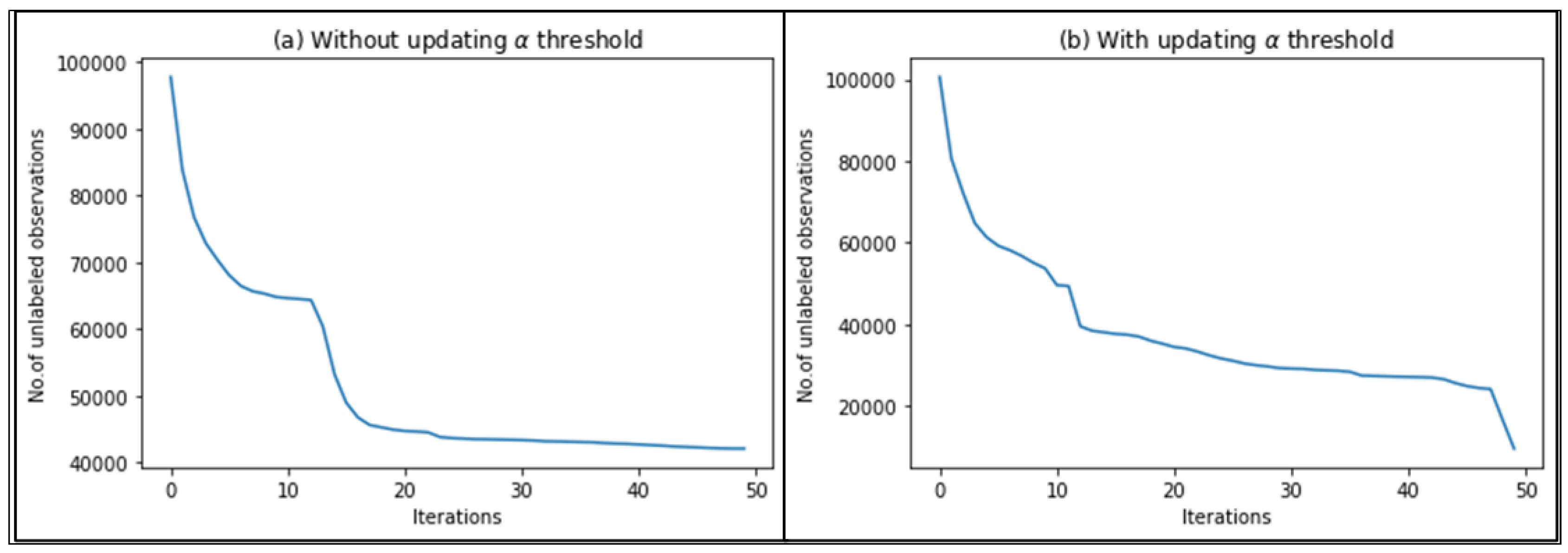
4.4.3. Optimisation of Threshold

Although practical IDSs are typically configured using multiple threshold parameters, choosing an appropriate threshold value can prove to be a challenging problem.

In our case, by tuning the threshold parameters, we could either maximize or minimize the accuracy and efficiency of the labeling process. To answer this question, we will investigate and analyze the impact of applying five values of $\alpha$ threshold ranging from 0.90 to 1, three values of $\beta$, and two values of $\gamma$ in the performance of the proposed approach. Thus, in our case, the model will be retrained 30 times.

$$5(\alpha -\mathrm{values})\ast 3(\beta -\mathrm{values})\ast 2(\gamma -\mathrm{values})=30$$

(15)

After we performing an exhaustive analysis, we conclude that the best set of parameters were ($\alpha =0.9,\beta =1.2\%,\gamma =0.01)$

4.5. Results and Discussion

Clearly, the proposed approach is intended to improve the accuracy of the labeling process using a small amount of labeled data to label a large unlabeled traffic data set. The accuracy results of the proposed approach is evaluated on multi-class datasets.

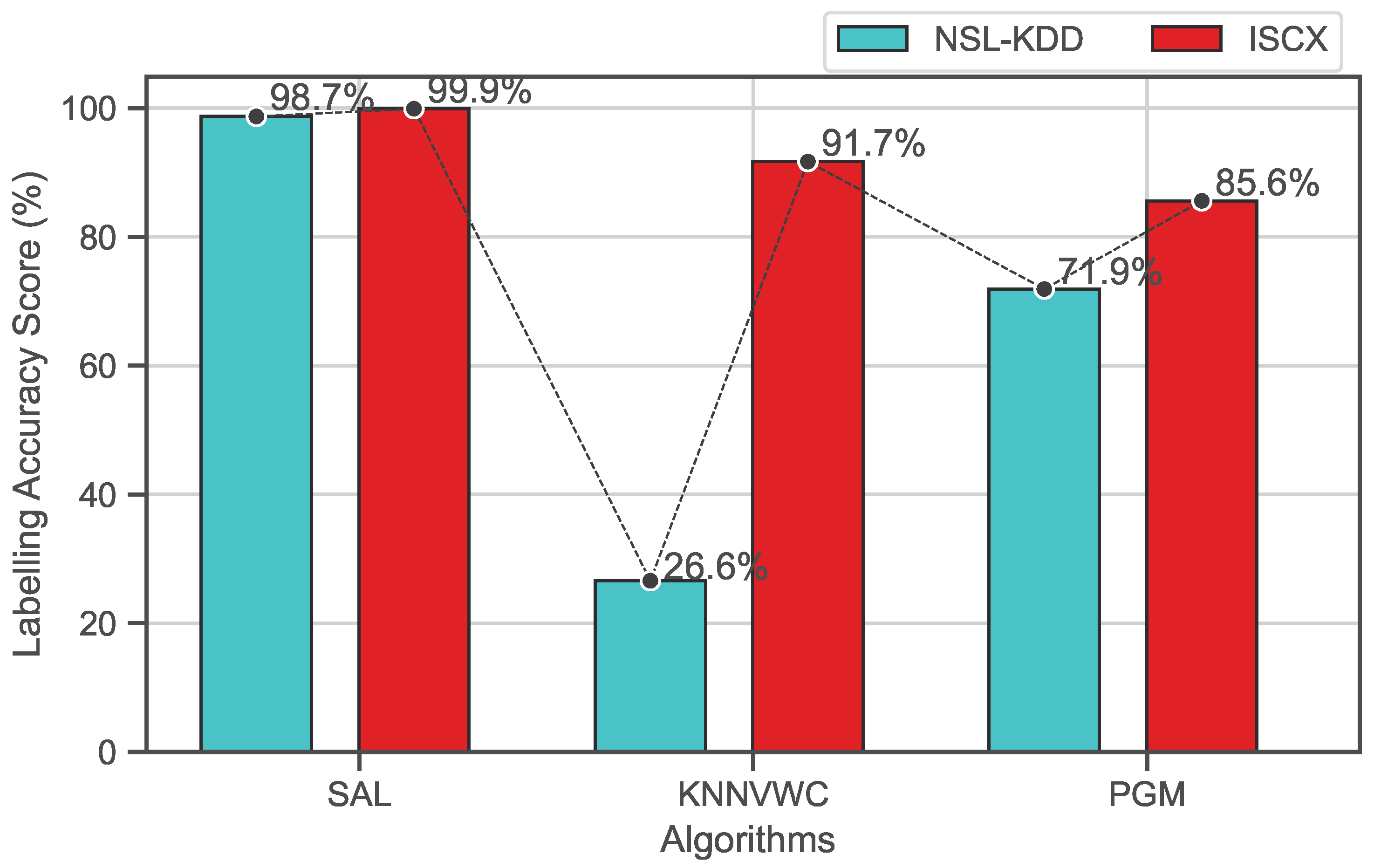
4.5.1. Overall Accuracy Evaluation

Figure 6 shows the overall accuracy of the proposed approach and the baseline algorithms on both NSL-KDD and ISCX data sets. As shown, the results demonstrate that the proposed approach SAL outperforms all baseline algorithms. Its overall accuracy scores are approximately (98.7%) for the NSL-KDD data set and (99.9%) for the ISCX data set, which are higher than kNNVWC and PGM, which record overall accuracies of (26.6%) and (71.9%) for the NSL-KDD data set and (91.7%) and (85.6%) for the ISCX data set, respectively.

We applied the Friedman test [38] followed by the Nemenyi posthoc test [39] to further investigate the overall accuracy of semi-supervised algorithms on both datasets. The former investigates the proposed approach as well as baseline algorithms across n data sets by ranking each model separately on each data set, so that rank 1 is assigned to the algorithm with the highest performance, rank 2 is assigned to the second highest, and so on. In the event of a tie, the average rank of all algorithms across all datasets is computed. In the latter test, the efficiency of the semi-supervised models is compared pairwise.

Figure 7 shows Friedman–Nemenyi test of the overall accuracy results with $(\alpha =0.05)$ on both datasets. The results indicate that the overall accuracy of SAL is scored the highest value (with rank 1) compared to the PGM and KNNVWC which have ranks 2 and 3, respectively.

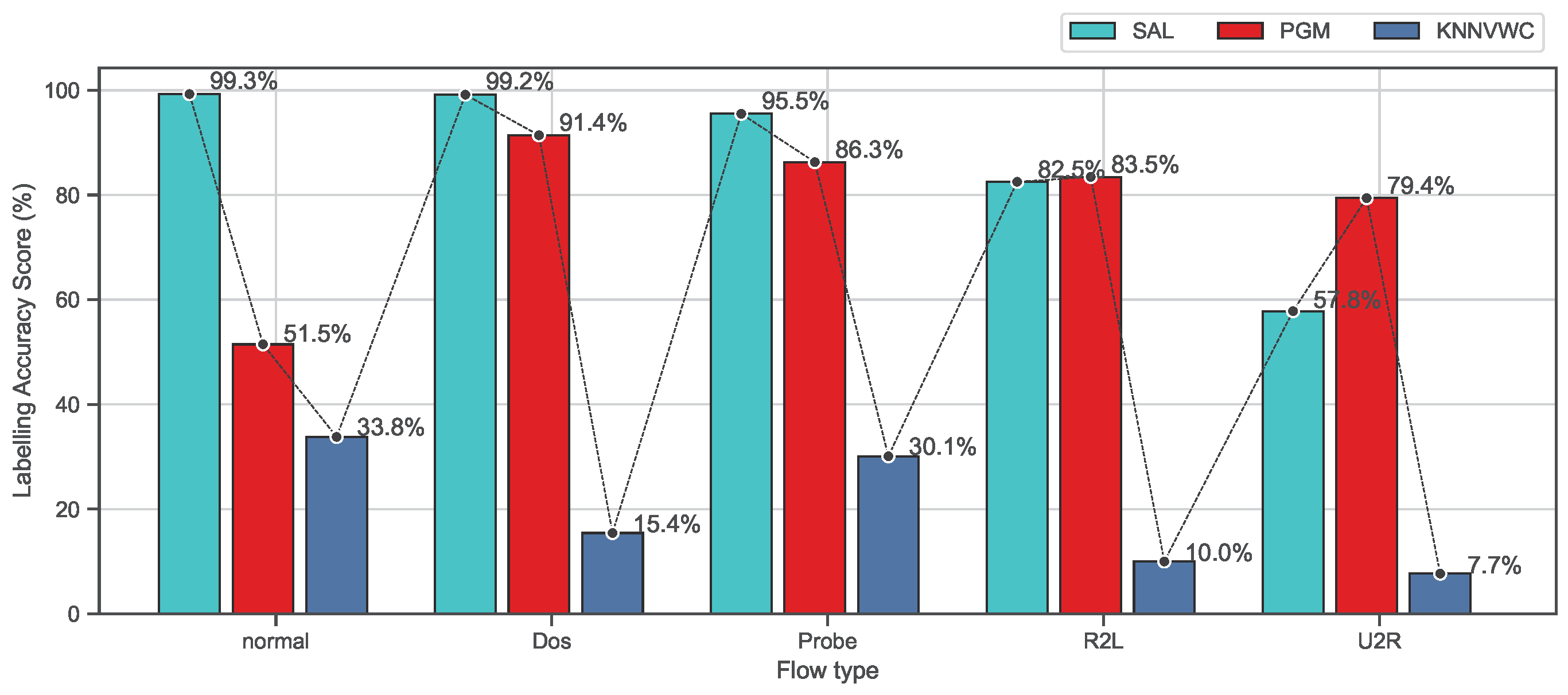
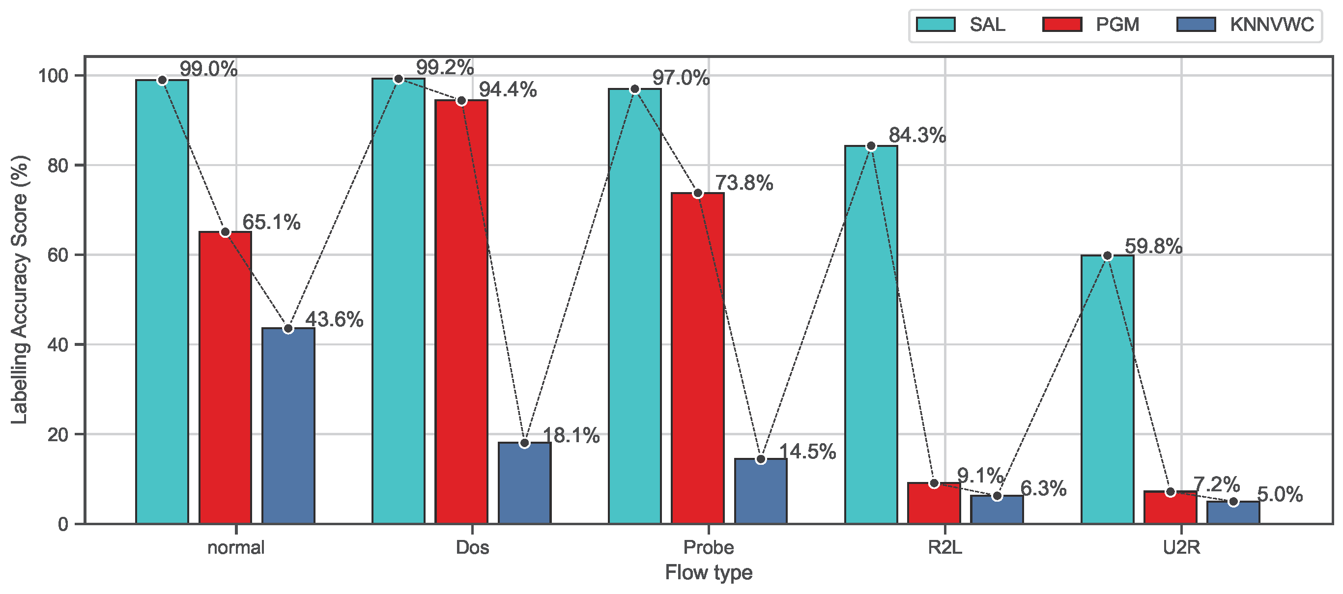
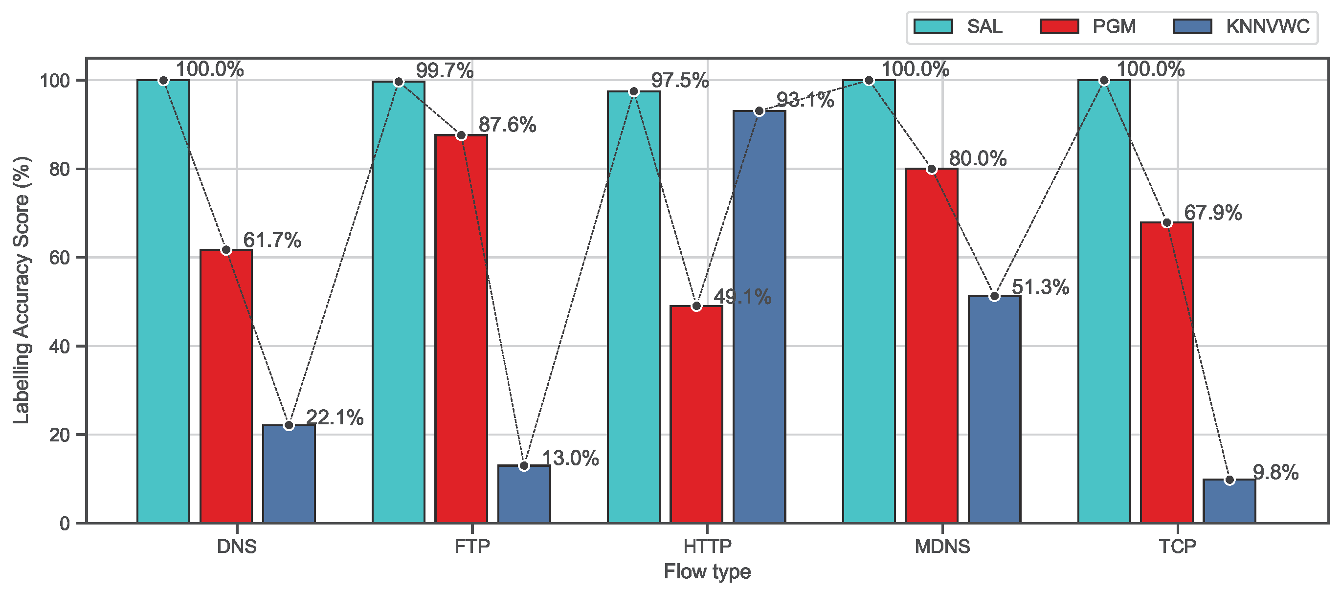
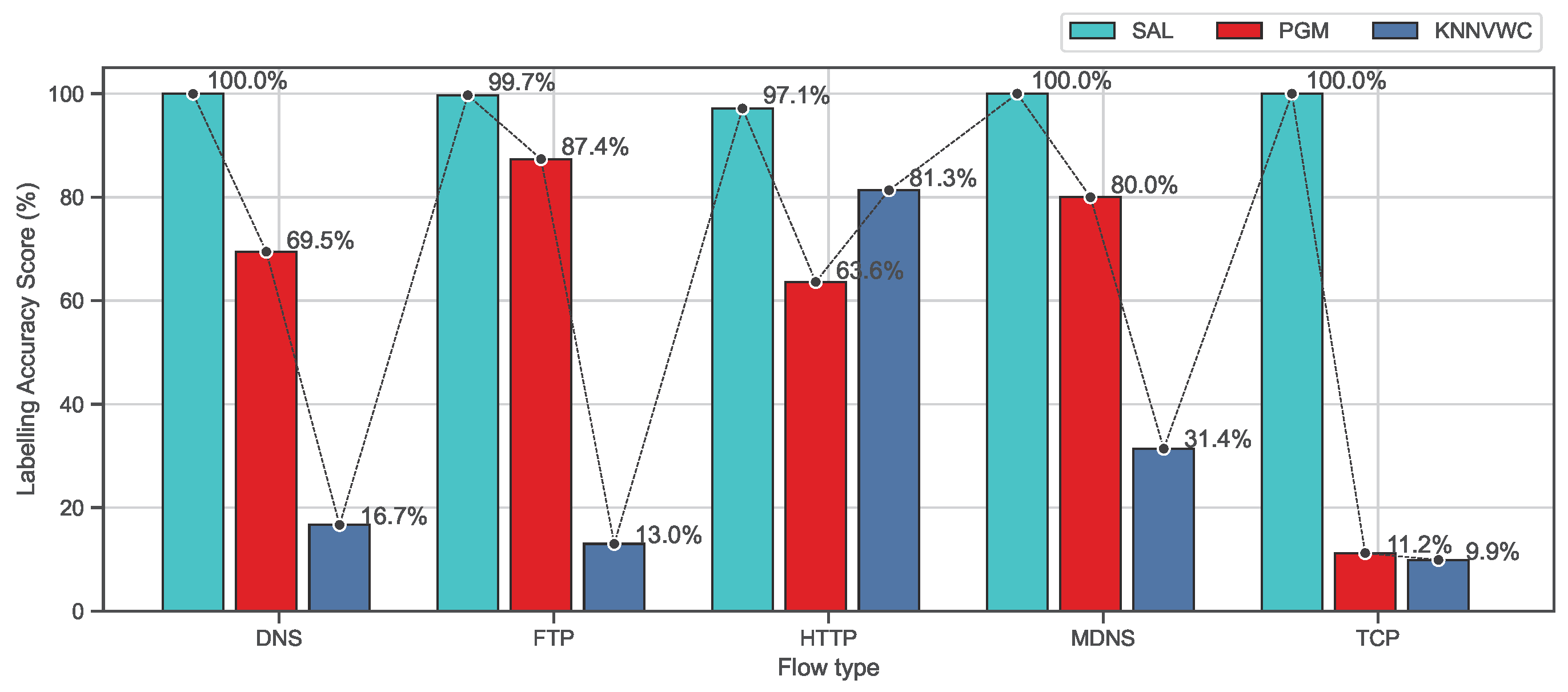
4.5.2. Class-Based Evaluation

Figure 8 and Figure 9 show the 10-fold cross-validation evaluation results of the labeling process using recall and F-measure metrics for each class separately on the NSL-KDD data set. As shown in Figure 8, this evaluation shows the comparison results of the proposed approach SAL and the baseline algorithms based on recall metric for each class. It can be seen that the proposed approach SAL consistently achieves the highest mean recall scores for labeling the normal, Dos, and probe classes, containing more than two values exceeding 95%, while PGM achieves the second highest mean recall, containing one value being above 90%. PGM achieves the highest mean recall results for R2L and U2L classes which are (83.46%) and (79.43%), respectively, while SAL obtains the second best mean recall (82.53%) and (57.82%). However, a labeling algorithm can obtain a high-precision score, while a number of observations are being missed (not labeled). Similarly, the algorithm can obtain a high recall score, while the false-positive rate is higher. Therefore, the F-measure, which is the harmonic mean of precision and recall, is a more appropriate metric to demonstrate the accuracy of the algorithm when working on classification models in which a data set is imbalanced. In the NSL-KDD data set, U2R and R2L attack types are relatively tiny fractions of the overall data set. Therefore, the proposed approach, as shown in Figure 9, demonstrates better accuracy results which are consistently higher than PGM and KNNVWC algorithms. From these results, we can conclude that the proposed approach SAL demonstrates promising results compared to baseline algorithms on the NSL-KDD data set. It can be concluded from the results that, under the assumption that the behaviour of abnormal activities mathematically or statistically differs from normal behaviours, or if they are noticeably distinguishable from the normal ones [40], the zero-day attacks can be classified as a attack type. This is because the proposed approach demonstrated significant results in differentiating among many flow types. This means the behaviour of the zero-day attacks will mathematically or statistically have similar characterisations as the known flow attack types.

Furthermore, Figure 10 and Figure 11 show the accuracy of the labeling process based on recall and F-measure metrics on the ISCX data set for the proposed approach and the baseline algorithms. As observed in Figure 10 and Figure 11, the proposed approach SAL significantly exceeds all baseline algorithms and the scores are always above 97% which is much higher than PGM and KNNVWC. These findings indicate that SAL is capable of dealing with a data set with high dimension and diverse distributions.

4.5.3. Runtime performance

Table 5. Runtime comparison of the three semi-supervised algorithms.

Datasets	SAL	KNNVWC	PGM
NSL-KDD	818.976 s	46.818 s	3.486 s
ISCX	6874.436 s	1052.318 s	36.96 s

captures the runtime performance of the three semi-supervised algorithms; the test was performed five times to obtain the mean execution time. From Table 5, it can be observed that the PGM is much faster than KNNVWC and SAL algorithms, respectively, in both datasets. Furthermore, when compared to the other two semi-supervised models, the runtimes of the SAL algorithm are the slowest. Therefore, future work will be reserved to minimise the runtime of the SAL approach.

5. Conclusions

The majority of existing machine learning-based intrusion detection systems (IDSs) rely on labeled predefined classes, which necessitate domain specialists to rapidly and effectively identify anomalies and threats. However, obtaining a reliable, up-to-date, and sufficient labeled data set for an efficient traffic intrusion detection model is extremely difficult. This paper presents a novel automatic labeling algorithm based on self-augmentation and ensemble classification strategies. The proposed SAL approach, in particular, has three phases: (1) an ensemble-based decision-making phase to address the limitations of a single classifier by aggregating the predictions of multi-classifiers, (2) a function agreement phase to assign a class label based on an adaptive confidence threshold to unlabeled observations, and (3) an increment update of an labeled set phase to maximize the accuracy and efficiency of the intrusion detection system classifier mode. In the experiments, two data sets of network traffic are used, which are collected from a variety of domains and are commonly used to evaluate anomaly detection systems. The experimental results show that the proposed SAL approach can accurately and efficiently detect and classify network traffic attacks and can outperform the performance of the baseline algorithms in terms of accuracy and F-score measurements. Future work will be reserved to minimise the run-time of the SAL approach since it can achieve the worst run time performance in the experiment.

References

1. Chio, C.; Freeman, D. Machine Learning and Security: Protecting Systems with Data and Algorithms; O’Reilly Media, Inc.: Sebastopol, CA, USA, 2018. [Google Scholar]
2. Al-Harthi, A. Designing an Accurate and Efficient Classification Approach for Network Traffic Monitoring. Ph.D. Thesis, RMIT University, Melbourne, Australia, 2015. [Google Scholar]
3. Taha, A.; Hadi, A.S. Anomaly Detection Methods for Categorical Data: A Review. ACM Comput. Surv. CSUR 2019, 52, 38. [Google Scholar] [CrossRef]
4. Bhattacharyya, D.K.; Kalita, J.K. Network Anomaly Detection: A Machine Learning Perspective; Chapman and Hall/CRC: Boca Raton, FL, USA, 2013. [Google Scholar]
5. Love, B.C. Comparing supervised and unsupervised category learning. Psychon. Bull. Rev. 2002, 9, 829–835. [Google Scholar] [CrossRef] [PubMed] [Green Version]
6. Erman, J.; Mahanti, A.; Arlitt, M.; Cohen, I.; Williamson, C. Offline/realtime traffic classification using semi-supervised learning. Perform. Eval. 2007, 64, 1194–1213. [Google Scholar] [CrossRef]
7. Rotsos, C.; Van Gael, J.; Moore, A.W.; Ghahramani, Z. Probabilistic graphical models for semi-supervised traffic classification. In Proceedings of the 6th International Wireless Communications and Mobile Computing Conference, Caen, France, 28 June–2 July 2010; pp. 752–757. [Google Scholar]
8. Marsland, S. Machine Learning: An Algorithmic Perspective; Chapman and Hall/CRC: Boca Raton, FL, USA, 2014. [Google Scholar]
9. Li, L.; Zhang, H.; Peng, H.; Yang, Y. Nearest neighbors based density peaks approach to intrusion detection. Chaos Solitons Fractals 2018, 110, 33–40. [Google Scholar] [CrossRef]
10. Xue, Y.; Jia, W.; Zhao, X.; Pang, W. An evolutionary computation based feature selection method for intrusion detection. Secur. Commun. Netw. 2018, 2018, 2492956. [Google Scholar] [CrossRef]
11. Gu, J.; Wang, L.; Wang, H.; Wang, S. A novel approach to intrusion detection using SVM ensemble with feature augmentation. Comput. Secur. 2019, 86, 53–62. [Google Scholar] [CrossRef]
12. Kabir, E.; Hu, J.; Wang, H.; Zhuo, G. A novel statistical technique for intrusion detection systems. Future Gener. Comput. Syst. 2018, 79, 303–318. [Google Scholar] [CrossRef] [Green Version]
13. Gao, L.; Li, Y.; Zhang, L.; Lin, F.; Ma, M. Research on Detection and Defense Mechanisms of DoS Attacks Based on BP Neural Network and Game Theory. IEEE Access 2019, 7, 43018–43030. [Google Scholar] [CrossRef]
14. Salo, F.; Nassif, A.B.; Essex, A. Dimensionality reduction with IG-PCA and ensemble classifier for network intrusion detection. Comput. Netw. 2019, 148, 164–175. [Google Scholar] [CrossRef]
15. Tan, H.; Gui, Z.; Chung, I. A Secure and Efficient Certificateless Authentication Scheme With Unsupervised Anomaly Detection in VANETs. IEEE Access 2018, 6, 74260–74276. [Google Scholar] [CrossRef]
16. Pan, Y.; Sun, F.; Teng, Z.; White, J.; Schmidt, D.C.; Staples, J.; Krause, L. Detecting web attacks with end-to-end deep learning. J. Internet Serv. Appl. 2019, 10, 1–22. [Google Scholar] [CrossRef] [Green Version]
17. Yao, H.; Fu, D.; Zhang, P.; Li, M.; Liu, Y. MSML: A Novel Multilevel Semi-Supervised Machine Learning Framework for Intrusion Detection System. IEEE Internet Things J. 2018, 6, 1949–1959. [Google Scholar] [CrossRef] [Green Version]
18. Mohammadi, S.; Mirvaziri, H.; Ghazizadeh-Ahsaee, M.; Karimipour, H. Cyber intrusion detection by combined feature selection algorithm. J. Inf. Secur. Appl. 2019, 44, 80–88. [Google Scholar] [CrossRef]
19. Song, H.; Jiang, Z.; Men, A.; Yang, B. A hybrid semi-supervised anomaly detection model for high-dimensional data. Comput. Intell. Neurosci. 2017, 2017, 8501683. [Google Scholar] [CrossRef] [Green Version]
20. Camacho, J.; Maciá-Fernández, G.; Fuentes-García, N.M.; Saccenti, E. Semi-supervised multivariate statistical network monitoring for learning security threats. IEEE Trans. Inf. Forensics Secur. 2019, 14, 2179–2189. [Google Scholar] [CrossRef] [Green Version]
21. Vercruyssen, V.; Wannes, M.; Gust, V.; Koen, M.; Ruben, B.; Jesse, D. Semi-supervised anomaly detection with an application to water analytics. In Proceedings of the IEEE International Conference on Data Mining, Singapore, 17–20 November 2018. [Google Scholar]
22. Idhammad, M.; Afdel, K.; Belouch, M. Semi-supervised machine learning approach for DDoS detection. Appl. Intell. 2018, 48, 3193–3208. [Google Scholar] [CrossRef]
23. Suaboot, J.; Fahad, A.; Tari, Z.; Grundy, J.; Mahmood, A.N.; Almalawi, A.; Zomaya, A.Y.; Drira, K. A Taxonomy of Supervised Learning for IDSs in SCADA Environments. ACM Comput. Surv. CSUR 2020, 53, 1–37. [Google Scholar] [CrossRef]
24. Dietterich, T.G. Ensemble methods in machine learning. In Proceedings of the International Workshop on Multiple Classifier Systems, Cagliari, Italy, 21–23 June 2000; pp. 1–15. [Google Scholar]
25. Mahabub, A. A robust technique of fake news detection using Ensemble Voting Classifier and comparison with other classifiers. SN Appl. Sci. 2020, 2, 1–9. [Google Scholar] [CrossRef] [Green Version]
26. Dietterich, T.G. Ensemble learning. Handb. Brain Theory Neural Netw. 2002, 2, 110–125. [Google Scholar]
27. Chen, C.O.; Zhuo, Y.Q.; Yeh, C.C.; Lin, C.M.; Liao, S.W. Machine learning-based configuration parameter tuning on hadoop system. In Proceedings of the 2015 IEEE International Congress on Big Data, New York, NY, USA, 27 June–2 July 2015; pp. 386–392. [Google Scholar]
28. Almalawi, A.M.; Fahad, A.; Tari, Z.; Cheema, M.A.; Khalil, I. k NNVWC: An Efficient k-Nearest Neighbors Approach Based on Various-Widths Clustering. IEEE Trans. Knowl. Data Eng. 2015, 28, 68–81. [Google Scholar] [CrossRef]
29. Bala, R.; Nagpal, R. A review on kdd cup99 and nsl nsl-kdd dataset. Int. J. Adv. Res. Comput. Sci. 2019, 10, 64–67. [Google Scholar] [CrossRef] [Green Version]
30. Shiravi, A.; Shiravi, H.; Tavallaee, M.; Ghorbani, A.A. Toward developing a systematic approach to generate benchmark datasets for intrusion detection. Comput. Secur. 2012, 31, 357–374. [Google Scholar] [CrossRef]
31. Mortaz, E. Imbalance accuracy metric for model selection in multi-class imbalance classification problems. Knowl.-Based Syst. 2020, 210, 106490. [Google Scholar] [CrossRef]
32. Kohavi, R. A study of cross-validation and bootstrap for accuracy estimation and model selection. In Proceedings of the International Joint Conference on Artificial Intelligence, Montreal, QC, Canada, 20–25 August 1995; Volume 14, pp. 1137–1145. [Google Scholar]
33. Pedregosa, F.; Varoquaux, G.; Gramfort, A.; Michel, V.; Thirion, B.; Grisel, O.; Blondel, M.; Prettenhofer, P.; Weiss, R.; Dubourg, V.; et al. Scikit-learn: Machine learning in Python. J. Mach. Learn. Res. 2011, 12, 2825–2830. [Google Scholar]
34. Shekar, B.; Dagnew, G. Grid search-based hyperparameter tuning and classification of microarray cancer data. In Proceedings of the 2019 Second International Conference on Advanced Computational and Communication Paradigms (ICACCP), Gangtok, India, 25–28 February 2019; pp. 1–8. [Google Scholar]
35. Parmar, A.; Katariya, R.; Patel, V. A review on random forest: An ensemble classifier. In International Conference on Intelligent Data Communication Technologies and Internet of Things; Springer: Berlin/Heidelberg, Germany, 2018; pp. 758–763. [Google Scholar]
36. Mathanker, S.; Weckler, P.; Bowser, T.; Wang, N.; Maness, N. AdaBoost classifiers for pecan defect classification. Comput. Electron. Agric. 2011, 77, 60–68. [Google Scholar] [CrossRef]
37. Moon, D.; Im, H.; Kim, I.; Park, J.H. DTB-IDS: An intrusion detection system based on decision tree using behavior analysis for preventing APT attacks. J. Supercomput. 2017, 73, 2881–2895. [Google Scholar] [CrossRef]
38. Friedman, M. A comparison of alternative tests of significance for the problem of m rankings. Ann. Math. Stat. 1940, 11, 86–92. [Google Scholar] [CrossRef]
39. Hollander, M.; Wolfe, D.A.; Chicken, E. Nonparametric Statistical Methods; John Wiley & Sons: Hoboken, NJ, USA, 2013; Volume 751. [Google Scholar]
40. Denning, D.E. An intrusion-detection model. IEEE Trans. Softw. Eng. 1987, SE-13, 222–232. [Google Scholar] [CrossRef]
Figure 1. General overview of the proposed framework.
Applsci 12 07189 g001
Figure 2. Hard ensemble voting algorithm.
Applsci 12 07189 g002
Figure 3. Soft ensemble voting algorithm.
Applsci 12 07189 g003
Figure 4. The proposed hybrid ensemble voting algorithm.
Applsci 12 07189 g004
Figure 5. Relation between the number of iterations and α .
Applsci 12 07189 g005
Figure 6. Overall accuracy comparison of semi-supervised algorithms on both datasets.
Applsci 12 07189 g006
Figure 7. Overall accuracy comparison of the three semi-supervised algorithms on the both datasets using the Friedman–Nemenyi test. (a) Overall accuracy on the NSL-KDD dataset. (b) Overall accuracy on the ISCX dataset.
Applsci 12 07189 g007
Figure 8. Comparison of labeling processes based on recall metrics on the NSL-KDD dataset.
Applsci 12 07189 g008
Figure 9. Comparison of labeling processes based on F-measure metrics on the NSL-KDD dataset.
Applsci 12 07189 g009
Figure 10. Comparison of labeling processes based on recall metrics on the ISCX dataset.
Applsci 12 07189 g010
Figure 11. Comparison of labeling processes based on F-measure metrics on the ISCX dataset.
Applsci 12 07189 g011