Review

DECIDE: A Deterministic Mixed Quantum-Classical Dynamics Approach

1
Department of Chemistry, University of Alberta, Edmonton, AB T6G 2G2, Canada
2
Dipartimento di Scienze Matematiche e Informatiche, Scienze Fisiche e Scienze della Terra, Università degli Studi di Messina, 98166 Messina, Italy
*
Author to whom correspondence should be addressed.
Current address: Department of Chemistry, University of Wisconsin-Madison, Madison, WI 53706, USA.
Appl. Sci. 2022, 12(14), 7022; https://doi.org/10.3390/app12147022
Submission received: 2 June 2022 / Revised: 30 June 2022 / Accepted: 6 July 2022 / Published: 12 July 2022
(This article belongs to the Special Issue Computer Simulation of Quantum and Classical Systems)

Abstract

:
Mixed quantum-classical dynamics provides an efficient way of simulating the dynamics of quantum subsystems coupled to many-body environments. Many processes, including proton-transfer reactions, electron-transfer reactions, and vibrational energy transport, for example, take place in such open systems. The most accurate algorithms for performing mixed quantum-classical simulations require very large ensembles of trajectories to obtain converged expectation values, which is computationally prohibitive for quantum subsystems containing even a few degrees of freedom. The recently developed “Deterministic evolution of coordinates with initial decoupled equations” (DECIDE) method has demonstrated high accuracy and low computational cost for a host of model systems; however, these applications relied on representing the equations of motion in subsystem and adiabatic energy bases. While these representations are convenient for certain systems, the position representation is convenient for many other systems, including systems undergoing proton- and electron-transfer reactions. Thus, in this review, we provide a step-by-step derivation of the DECIDE approach and demonstrate how to cast the DECIDE equations in a quantum harmonic oscillator position basis for a simple one-dimensional (1D) hydrogen bond model. After integrating the DECIDE equations of motion on this basis, we show that the total energy of the system is conserved for this model and calculate various quantities of interest. Limitations of casting the equations in an incomplete basis are also discussed.

1. Introduction

Most systems of interest in chemistry and biology contain very large numbers of degrees of freedom (DOF). An exact simulation of the dynamics of such a system requires a fully quantum mechanical treatment of the entire system, which is computationally prohibitive due to the exponential scaling with the number of DOF. One approach to overcoming this issue is to treat a few DOF of interest quantum mechanically (i.e., subsystem) and the remainder classically (i.e., environment or bath) [1,2,3,4]. Within this approach, the quantum subsystem is described in terms of a Hilbert space and the classical environment in terms of a phase space of positions and momenta. Situations in which the quantum subsystem is described by a non-Hermitian Hamiltonian have also been considered [5]. Previously, these mixed quantum-classical techniques have been applied to a wide range of phenomena, e.g., proton transfer reactions [6,7], electron transfer reactions [8,9], proton-coupled electron transfer reactions [10,11,12,13,14,15,16], exciton transport in photosynthetic complexes [17,18,19], heat transport in molecular junctions [20,21,22,23,24], metamolecules [25], and magnetic molecules [26,27].
The quantum-classical Liouville equation (QCLE) has served as a starting point for simulating the dynamics of mixed quantum-classical systems [2,28,29]. Over the years, a host of techniques have been developed based on approximate solutions of the QCLE [3,30]. The most accurate of these techniques are the stochastic surface-hopping solutions [6,31,32,33,34,35,36], but they require extremely large ensembles of trajectories to obtain converged results and, as a result, will be computationally prohibitive for many systems. On the other hand, the Poisson Bracket Mapping Equation (PBME) approach provides a highly computationally efficient approximate solution of the QCLE, but its applicability is mainly restricted to systems with weak subsystem-bath couplings [8,37,38,39]. Recently, the “Deterministic evolution of coordinates with initial decoupled equations” (DECIDE) method was developed, which offers a favourable balance between computational economy and accuracy [40]. DECIDE has two main advantages compared to the stochastic QCLE-based methods: (i) It is a deterministic method that requires the integration of L 2 ( L 2 2 + 2 N ) coupled differential equations (where L is the number of basis functions used to represent the subsystem and N is the number of environmental DOF). Typically, only a few thousand trajectories are required to obtain converged results, in contrast to several orders of magnitude more trajectories in the case of the stochastic QCLE-based methods; (ii) There is no need to diagonalize the Hamiltonian matrix on-the-fly. DECIDE has demonstrated great promise in solving the QCLE with high accuracy and low computational cost for a number of model systems, including the spin-boson model [40,41], Fenna–Matthews–Olson model [40,41], a three-state photo-induced electron transfer model [40], nonequilibrium spin-boson model [21,22,42], and a quantum battery model [43].
To date, the DECIDE equations have been represented in complete spin, subsystem, and adiabatic energy bases and successfully applied to simulate the dynamics of Hamiltonians expressed in these bases. However, the feasibility of solving the DECIDE equations in an incomplete position basis has yet to be explored. In this review, we explore this by first considering a one-dimensional, quadratic model of a hydrogen bond coupled to a solvent coordinate.
The review is organized as follows. In Section 2, we first discuss the Wigner–Weyl transform, which has been widely used in mixed quantum-classical dynamics, as it provides an invertible mapping between Hilbert space operators and phase space functions. In Section 3, we derive the DECIDE equations of motion and briefly discuss their underlying approximations and energy conservation. In Section 4, we provide a practical demonstration of how to implement the DECIDE approach using an incomplete position basis by considering a simple one-dimensional hydrogen bond model. We also briefly discuss issues that may arise when representing the DECIDE equations of motion for an arbitrary system in an incomplete basis. Finally, we summarize the main points of this review and discuss a future direction in Section 5.

2. Wigner-Weyl Transform

Before deriving the DECIDE equations of motion, we present an overview of the Wigner–Weyl transform and its properties. The Wigner–Weyl transform, which was first introduced by Wigner in 1932 [44], is a starting point for deriving mixed quantum-classical dynamics methods. Wigner’s original goal was to find correction terms that would bridge quantum and classical mechanics [44,45].
The transform can be understood in terms of probability functions. For a wave function expressed in position space, ψ ( x ) , the probability density is | ψ ( x ) | 2 . The wave function can also be expressed in momentum space as
ϕ ( p ) = 1 h e i x p / ψ ( x ) d x p | ψ ,
and its associated probability density is | ϕ ( p ) | 2 ( = h / 2 π and h is Planck’s constant). Each probability density above depends on either x or p. The Wigner–Weyl transform provides a way to represent the probability distribution in terms of both position ( x ) and momentum ( p ) . By definition, the Wigner–Weyl transform of an operator A ^ is
A W ( x , p ) = e i p y / ψ * ( x + y 2 ) A ^ ψ ( x y 2 ) d y , e i p y / x + y 2 | A ^ | x y 2 d y ,
where x and p are vectors containing the positions and momenta of all DOF in the system and y is an arbitrary integration variable.
Using the above definition, one can obtain several properties of this transform. First, the identity operator 1 ^ is given by
1 W = e i p y / x + y 2 | 1 ^ | x y 2 d y = e i p y / δ ( x + y 2 x + y 2 ) d y = 1 .
Second, for an operator A ^ that is only a function of the position operator x ^ , the Wigner–Weyl transform is
e i p y / x + y 2 | A ^ | x y 2 d y = e i p y / A ( x y 2 ) δ ( y ) d y = A ( x ) .
Similarly, for an operator A ^ that is only a function of p ^ , its Wigner–Weyl transform is A ( p ) . Third, the trace of the product of two operators A ^ and B ^ is
Tr ( A ^ B ^ ) = 1 h A W ( x , p ) B W ( x , p ) d x d p .
The Wigner function W ( x , p ) , which corresponds to the probability density of x and p, is defined in terms of the Wigner transform of the density operator ρ ^ = | ψ ψ | as
ρ W ( x , p ) h = 1 h e i p y | x + y 2 x y 2 | d x d y W ( x , p ) .
For example, the Wigner functions for the ground and first-excited states of the quantum harmonic oscillator are shown in Figure 1.
In the Wigner–Weyl representation, the expectation value of an operator A ^ is given by
A ^ = Tr ( ρ ^ A ^ ) = W ( x , p ) A W ( x , p ) d x d p ,
where W ( x , p ) is normalized, i.e.,
W ( x , p ) d x d p = Tr ( ρ ) = 1 .
The Wigner–Weyl transform of the product of two operators is [46]
( A ^ B ^ ) W = A W ( x , p ) exp ( Λ / 2 i ) B W ( x , p ) A W ( x , p ) * B W ( x , p ) .
In the above equation, * denotes the Moyal star product [47,48] and Λ is the Poisson bracket operator,
Λ = p · x x · p ,
where an arrow denotes the direction of the operation. (The derivation of Equation (9) may be found in Ref. [46].) The exponential in Equation (9) may be expanded in the following series,
e Λ / 2 i = 1 + 2 i Λ + 2 i Λ 2 / 2 ! + .

3. DECIDE Mixed Quantum-Classical Dynamics

In this section, we derive the DECIDE equations of motion [40]. Let us start by considering a fully quantum system with a time-independent Hamiltonian H ^ = H ^ S ( x ^ ) + H ^ B ( X ^ ) + H ^ C ( x ^ , X ^ ) , where H ^ S is the subsystem Hamiltonian, H ^ B is the bath Hamiltonian, H ^ C is the subsystem-bath coupling Hamiltonian, x ^ denotes a set of generalized coordinates that provides a complete description of the state of the subsystem, and X ^ = ( R ^ , P ^ ) denotes the set of position and momentum operators of the bath. In the Heisenberg picture, the dynamics of the subsystem and bath coordinates are given by the quantum Liouville equation, namely
d d t x ^ ( t ) = i H ^ , x ^ ( t ) = i e i L ^ t H ^ , x ^ i H ^ , x ^ ( t ) d d t X ^ ( t ) = i H ^ , X ^ ( t ) = i e i L ^ t H ^ , X ^ i H ^ , X ^ ( t ) ,
where e i L ^ t A ^ = e i H ^ t / A ^ e i H ^ t / . In the above equations, the time arguments outside the brackets indicate that one should first evaluate the commutator, then apply the time dependence. Taking a partial Wigner transform over the bath DOF (defined in terms of the bath DOF at t = 0 ) of the above equations and retaining only zero-order terms in in the resulting Moyal product expansion yields,
d d t ( x ^ ( t ) ) W = i e i L ^ t W e Λ / 2 i H ^ , x ^ W i e i L ^ W t H ^ , x ^ W d d t ( X ^ ( t ) ) W i e i L ^ W t H ^ , X ^ W ,
Assuming that the subsystem and bath coordinates are initially decoupled, evaluating the partial Wigner transform of the commutators in the above equations, and retaining only first-order terms in in the resulting Moyal product expansion leads to the DECIDE equations of motion,
d d t ( x ^ ( t ) ) W i e i L ^ W t H ^ W , x ^ = i H ^ W , x ^ ( t ) d d t ( X ^ ( t ) ) W e i L ^ W t H ^ W , X a = H ^ W , X a ( t ) ,
where the antisymmetrized Poisson bracket is given by { H ^ W , A ^ W } a = 1 2 { H ^ W , A ^ W } 1 2 { A ^ W , H ^ W } . (N.B.: The assumption that the subsystem and bath are initially decoupled leads to ( [ H ^ , x ^ ] ) W = [ H ^ W , x ^ ] and ( [ H ^ , X ^ ] ) W = i { H ^ W , X ^ } a .) It should be noted that the partially Wigner-transformed Hamiltonian retains an operator character because the transform was not performed on the subsystem DOF. In addition, to account for noncommutativity in the above equations, one has to replace any coupling terms in H C with their Weyl-ordered symmetric forms, e.g., x ^ X would be replaced by 1 2 ( x ^ X + X x ^ ) . The errors caused by the approximations above become significant when the subsystem dynamics is highly non-Markovian, namely when the dependence on the initial bath coordinates is important [40]. This can be the case for very low bath temperatures, very strong subsystem-bath coupling, and very slow baths, i.e., when memory effects are very pronounced [22,40].
The general form of the partially Wigner-transformed Hamiltonian considered in the next section is given by
H ^ W ( R , P ) = P 2 2 M + p ^ 2 2 m + V ^ W ( r ^ , R ) ,
where r ^ and p ^ are vectors containing the subsystem position and momentum operators, respectively, and m and M are vectors containing the masses of the subsystem and bath DOF, respectively. For this form of Hamiltonian, the DECIDE equations of motion for the subsystem and bath DOF are
d r ^ d t = i H ^ W , r ^ = p ^ m , d p ^ d t = i H ^ W , p ^ = V ^ W r ^ . d R d t = H ^ W , R = H ^ W P · R R H ^ W R · R P = P m , d P d t = H ^ W , P = V ^ W R .
Finally, one must select a convenient basis for the quantum subsystem to solve these equations.
To show that the total energy of the system is conserved over the course of the dynamics, we start by taking the time derivative of a matrix element (in any basis) of the Hamiltonian, i.e.,
d H W α α d t = H ^ W r ^ d r ^ d t + H ^ W p ^ d p ^ d t + H ^ W R d R d t + H ^ W P d P d t α α ,
where H α α = α | H ^ W | α . Substituting the expressions for the time derivatives of the subsystem and bath DOFs in Equation (16) into Equation (17), we find that
d H W α α d t = 0 ,
thereby proving that the energy of the total system is conserved.

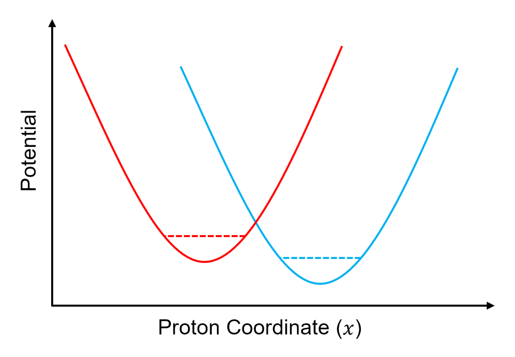
4. Hydrogen Bond Model

We now demonstrate how to implement the DECIDE approach using an incomplete position basis by considering a simple, quadratic, 1D hydrogen bond model.

4.1. Model

The Weyl-ordered, partially Wigner-transformed Hamiltonian of the hydrogen bond model is given by
H ^ W = p ^ 2 2 m + P 2 2 M + A 0 x ^ 2 + 1 2 k 1 X x ^ + 1 2 k 1 x ^ X ,
where x ^ / p ^ is the position/momentum operator of the proton, X / P is the position/momentum of the solvent coordinate, and A 0 and k 1 are constants. Plots of the protonic potential for two values of X are shown in Figure 2.
A convenient basis for solving this proton transfer problem is a set of quantum harmonic oscillator wave functions, i.e.,
ϕ n ( x ) = x | ϕ n = ( 2 n n ! π ) 1 / 2 b 1 / 2 H n ( b x ) exp [ b 2 x 2 / 2 ] ,
where H n is the nth Hermite polynomial, b is an arbitrary constant, and n = 0 , 1 , 2 , . Note that if X = 0 in Equation (19), then the exact solution of the time-independent Schrödinger equation for this model is ϕ n ( x ) with b = 2 m A 0 / 2 1 / 4 . In our simulations, we take b = 8 m A 0 / 2 1 / 4 . The eigenfunctions of H ^ W may be expanded in this basis as | ψ i = n c n i | ϕ n , where c n i is the coefficient of the nth basis function. For this expansion, we use 12 basis functions ( n = 0 , , 11 ). Substituting the eigenfunction expansion into the time-independent Schrödinger equation, we obtain an eigenvalue problem of the form H c = c E , where H is the Hamiltonian matrix expressed in the chosen basis, c is a matrix containing the c n i ’s of the ith eigenfunction, and E is a diagonal matrix containing the eigenvalues E i ( X ) . The Hamiltonian matrix elements are calculated by numerical integration, and the eigenvalue problem is solved (to obtain the c n i ’s and eigenvalues) using built-in functions in MATLAB. Figure 3 shows the ground- and first-excited state adiabatic potential energy surfaces [ E 0 ( X ) and E 1 ( X ) , respectively] calculated using this method.
It turns out that the time-independent Schrödinger equation for the Hamiltonian in Equation (19) can be solved analytically (and exactly) by first rewriting the potential energy as A 0 ( x + k 1 2 A 0 X x ) 2 k 1 2 4 A 0 X 2 . The resulting adiabatic energies are
E n ( X ) = 2 A 0 m ( n + 1 2 ) k 1 2 4 A 0 X 2 , n = 0 , 1 , 2 , 3 ,
where n labels the energy level. Comparing our variational results to the exact ones, we find that good agreement is obtained when X is close to 0, but differences emerge when | X | > 0.25 (see Figure 3). The convergence of the variational result can be improved by increasing the number of basis functions; however, the level of accuracy achieved with 12 basis functions is sufficient for our purposes.

4.2. Dynamics Simulation Details
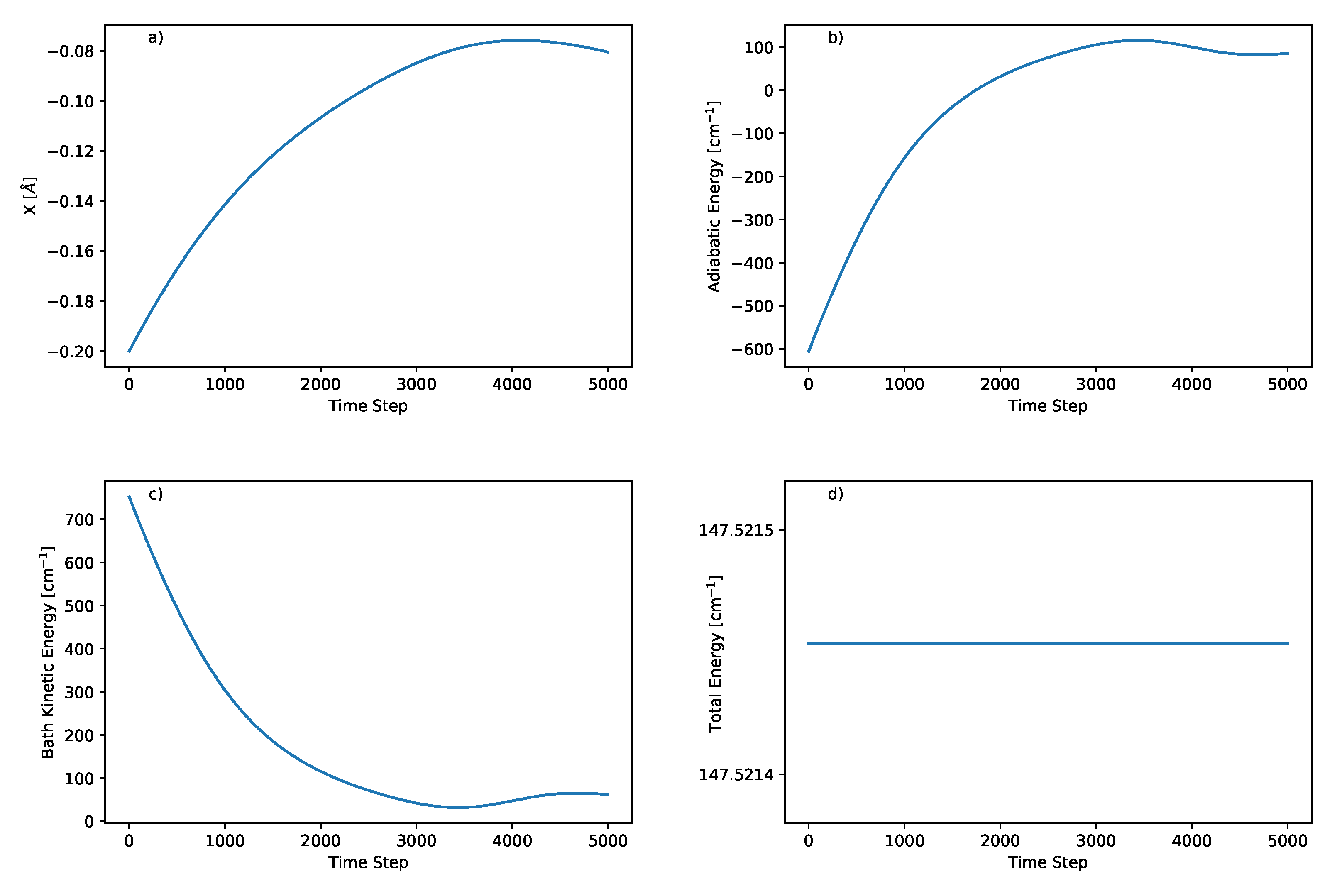
Using Equation (16) and the Hamiltonian in Equation (19), one may obtain the DECIDE equations of motion for the proton transfer model in the quantum harmonic oscillator basis, viz.,
d d t x α α ( t ) = i [ H ^ W , x ^ ] α α = p α α m d d t p α α ( t ) = i [ H ^ W , p ^ ] α α = A 0 x α α k 1 X α α d d t X α α ( t ) = { H ^ W , X } α α = P α α m d d t P α α ( t ) = { H ^ W , P } α α = k 1 x α α ,
where, for example, x α α = α | x ^ | α and | α is the α t h harmonic oscillator state. Given that the basis set is composed of 12 functions, the total number of coupled differential equations is 12 2 × 4 .
We assume the initial state of the composite system to be factorized, i.e., ρ ^ ( 0 ) = ρ ^ S ( 0 ) ρ B , W ( 0 ) , where ρ ^ S ( 0 ) is the initial density operator of the subsystem (viz., the proton) and ρ B , W ( 0 ) is the initial Wigner distribution of the bath (viz., the solvent coordinate). In our simulations, the system is initialized in the adiabatic ground state | ψ 0 of the Hamiltonian in Equation (19), such that ρ ^ S ( t ) = | ψ 0 ψ 0 | . In the harmonic oscillator basis, the initial values of the matrix elements of the subsystem coordinates are given by the following analytical expressions:
x α α ( 0 ) = 1 2 2 / 2 m A 0 1 / 4 α + 1 δ α + 1 , α + α + 1 δ α , α + 1 , p α α ( 0 ) = i 2 2 m A 0 1 / 4 α + 1 δ α + 1 , α α + 1 δ α , α + 1 .
The initial values of the matrix elements of the bath coordinates are given by
X α α ( 0 ) = X ( 0 ) δ α , α , P α α ( 0 ) = P ( 0 ) δ α , α ,
where X ( 0 ) / P ( 0 ) is the initial value of the bath position/momentum. In practice, X ( 0 ) and P ( 0 ) may be sampled from Wigner distributions corresponding to thermal equilibrium states. However, in this study, we choose X ( 0 ) = 0.2 Å and P ( 0 ) = 50 a.u., since we only generate a single trajectory for demonstration purposes. Starting from these initial conditions, the DECIDE equations of motion in Equation (22) are integrated using the Runge Kutta fourth-order method [49] with a time step of 1 a.u. to simulate the dynamics of the system. In general, a particular integrator is chosen to achieve an optimal balance between efficiency and accuracy for a given system.
The expectation value of a property A ^ ( t ) may be calculated according to
A ^ ( t ) = β β d X ( 0 ) d P ( 0 ) A β β ( t ) ρ S β β ( 0 ) ρ B , W ( 0 ) .
However, since we only consider single trajectories for this demonstration, we take ρ B , W ( 0 ) = 1 . In particular, we are interested in the conservation of the total energy along a trajectory, which is calculated according to
H ^ ( t ) = α α H α α ( t ) ρ S α α ( 0 ) .

4.3. Results

Figure 4 shows the values of X, adiabatic energy, bath kinetic energy, and total energy along a representative trajectory. For a positive initial momentum P ( 0 ) , we see that X increases up to about 4000 time steps and then starts to decrease. The adiabatic energy increases while the bath kinetic energy decreases over the course of this trajectory. Finally, as seen in Figure 4d, the total energy of the system is well-conserved along this trajectory.

4.4. Limitations of Position Representation

Although the DECIDE method is capable of accurately solving the 1D quadratic hydrogen bond model, problems in energy conservation may arise when integrating the DECIDE equations of motion for more complex models. A detailed analysis has revealed (results not shown) that a breakdown in energy conservation could occur due to a combination of basis set incompleteness (inherent to the position representation) and the presence of higher-order (i.e., cubic, quartic, etc.) terms in the Hamiltonian. In the DECIDE equations of motion, matrix elements of second or higher powers of the coordinates [e.g., ( x 2 ) α α ] are not evolved directly. Since only matrix elements of the first powers of the coordinates are evolved directly, the matrix elements of higher-order terms are evaluated by first inserting complete sets of states between each linear term in the product (e.g., ( x 2 ) α α = β x α β x β α ). Therefore, if the position basis is incomplete, such terms can be evaluated inaccurately, which leads to an accumulation of numerical errors and, in turn, a breakdown in energy conservation. In this connection, even in the 1D quadratic hydrogen bond model, there will be small numerical errors when calculating energies due to the presence of x 2 and p 2 terms in the Hamiltonian [see Equation (19)].

5. Conclusions

Mixed quantum-classical dynamics is a useful approach for simulating the dynamics of quantum processes occurring in chemical and biological systems with large numbers of DOF. Among the various mixed quantum-classical dynamics methods, the DECIDE method has exhibited a highly favourable balance between computational cost and accuracy for treating model Hamiltonians expressed in complete energy bases.
In this review, we explained the DECIDE method and demonstrated it on a 1D quadratic model of a proton in a hydrogen bond. This required casting the DECIDE equations of motion in an incomplete quantum harmonic oscillator position basis. We showed that with a sufficiently large basis, it is possible to generate trajectories that conserve the total energy of the system well. However, for higher-order models expressed in an incomplete position basis, energy conservation may break down and thus, it would be necessary to re-express the Hamiltonian in an energy basis. This approach will be explored in a future study.

Author Contributions

Conceptualization, Z.L., A.S. and G.H.; methodology, Z.L. and G.H.; software, Z.L.; validation, Z.L. and G.H.; formal analysis, Z.L. and G.H.; investigation, Z.L., A.S. and G.H.; resources, G.H.; data curation, Z.L.; writing—original draft preparation, Z.L. and G.H.; writing—review and editing, Z.L., A.S. and G.H.; supervision, G.H.; project administration, G.H. All authors have read and agreed to the published version of the manuscript.

Funding

This research was funded by the Natural Sciences and Engineering Research Council of Canada (NSERC).

Institutional Review Board Statement

Not applicable.

Informed Consent Statement

Not applicable.

Data Availability Statement

Not applicable.

Conflicts of Interest

The authors declare no conflict of interest.

Abbreviations

The following abbreviations are used in this manuscript:
DECIDEDeterministic evolution of coordinates with initial decoupled equations
DOFDegrees of freedom
QCLEQuantum-classical Liouville equation
1DOne-dimensional

References

  1. Tully, J.C. Mixed quantum-classical dynamics. Faraday Discuss. 1998, 110, 407–419. [Google Scholar] [CrossRef]
  2. Kapral, R.; Ciccotti, G. Mixed quantum-classical dynamics. J. Chem. Phys. 1999, 110, 8919–8929. [Google Scholar] [CrossRef]
  3. Kapral, R. Progress in the theory of mixed quantum-classical dynamics. Annu. Rev. Phys. Chem. 2006, 57, 129–157. [Google Scholar] [CrossRef] [PubMed] [Green Version]
  4. Sergi, A.; Hanna, G.; Grimaudo, R.; Messina, A. Quasi-Lie brackets and the breaking of time-translation symmetry for quantum systems embedded in classical baths. Symmetry 2018, 10, 518. [Google Scholar] [CrossRef] [Green Version]
  5. Sergi, A. Embedding quantum systems with a non-conserved probability in classical environments. Theor. Chem. Accounts 2015, 134, 79. [Google Scholar] [CrossRef] [Green Version]
  6. Hanna, G.; Kapral, R. Quantum-classical Liouville dynamics of nonadiabatic proton transfer. J. Chem. Phys. 2005, 122, 244505. [Google Scholar] [CrossRef]
  7. Hammes-Schiffer, S.; Tully, J.C. Proton transfer in solution: Molecular dynamics with quantum transitions. J. Chem. Phys. 1994, 101, 4657–4667. [Google Scholar] [CrossRef] [Green Version]
  8. Rekik, N.; Hsieh, C.Y.; Freedman, H.; Hanna, G. A mixed quantum-classical Liouville study of the population dynamics in a model photo-induced condensed phase electron transfer reaction. J. Chem. Phys. 2013, 138, 144106. [Google Scholar] [CrossRef]
  9. Shakib, F.A.; Hanna, G. New insights into the nonadiabatic state population dynamics of model proton-coupled electron transfer reactions from the mixed quantum-classical Liouville approach. J. Chem. Phys. 2016, 144, 024110. [Google Scholar] [CrossRef]
  10. Fang, J.Y.; Hammes-Schiffer, S. Proton-coupled electron transfer reactions in solution: Molecular dynamics with quantum transitions for model systems. J. Chem. Phys. 1997, 106, 8442–8454. [Google Scholar] [CrossRef] [Green Version]
  11. Fang, J.Y.; Hammes-Schiffer, S. Excited state dynamics with nonadiabatic transitions for model photoinduced proton-coupled electron transfer reactions. J. Chem. Phys. 1997, 107, 5727–5739. [Google Scholar] [CrossRef] [Green Version]
  12. Fang, J.Y.; Hammes-Schiffer, S. Nonadiabatic dynamics for processes involving multiple avoided curve crossings: Double proton transfer and proton-coupled electron transfer reactions. J. Chem. Phys. 1997, 107, 8933–8939. [Google Scholar] [CrossRef] [Green Version]
  13. Soudackov, A.V.; Hammes-Schiffer, S. Removal of the double adiabatic approximation for proton-coupled electron transfer reactions in solution. Chem. Phys. Lett. 1999, 299, 503–510. [Google Scholar] [CrossRef]
  14. Shakib, F.A.; Hanna, G. An analysis of model proton-coupled electron transfer reactions via the mixed quantum-classical Liouville approach. J. Chem. Phys. 2014, 141, 044122. [Google Scholar] [CrossRef]
  15. Shakib, F.; Hanna, G. Mixed quantum-classical Liouville approach for calculating proton-coupled electron-transfer rate constants. J. Chem. Theory Comput. 2016, 12, 3020–3029. [Google Scholar] [CrossRef]
  16. Sayfutyarova, E.R.; Goings, J.J.; Hammes-Schiffer, S. Electron-coupled double proton transfer in the Slr1694 BLUF photoreceptor: A multireference electronic structure study. J. Phys. Chem. B 2018, 123, 439–447. [Google Scholar] [CrossRef]
  17. Panitchayangkoon, G.; Voronine, D.V.; Abramavicius, D.; Caram, J.R.; Lewis, N.H.; Mukamel, S.; Engel, G.S. Direct evidence of quantum transport in photosynthetic light-harvesting complexes. Proc. Natl. Acad. Sci. USA 2011, 108, 20908–20912. [Google Scholar] [CrossRef] [Green Version]
  18. Kelly, A.; Rhee, Y.M. Mixed quantum-classical description of excitation energy transfer in a model Fenna-Matthews-Olsen complex. J. Phys. Chem. Lett. 2011, 2, 808–812. [Google Scholar] [CrossRef]
  19. Harush, E.Z.; Dubi, Y. Do photosynthetic complexes use quantum coherence to increase their efficiency? Probably not. Sci. Adv. 2021, 7, eabc4631. [Google Scholar] [CrossRef]
  20. Segal, D.; Agarwalla, B.K. Vibrational heat transport in molecular junctions. Annu. Rev. Phys. Chem. 2016, 67, 185–209. [Google Scholar] [CrossRef] [Green Version]
  21. Liu, J.; Hsieh, C.Y.; Segal, D.; Hanna, G. Heat transfer statistics in mixed quantum-classical systems. J. Chem. Phys. 2018, 149, 224104. [Google Scholar] [CrossRef]
  22. Carpio-Martínez, P.; Hanna, G. Nonequilibrium heat transport in a molecular junction: A mixed quantum-classical approach. J. Chem. Phys. 2019, 151, 074112. [Google Scholar] [CrossRef]
  23. Kelly, A. Mean field theory of thermal energy transport in molecular junctions. J. Chem. Phys. 2019, 150, 204107. [Google Scholar] [CrossRef]
  24. Grimaldi, A.; Sergi, A.; Messina, A. Evolution of a non-Hermitian quantum single-molecule junction at constant temperature. Entropy 2021, 23, 147. [Google Scholar] [CrossRef]
  25. Uken, D.A.; Sergi, A. Quantum dynamics of a plasmonic meta-molecule with a time-dependent driving. Theor. Chem. Acc. 2015, 134, 141. [Google Scholar] [CrossRef] [Green Version]
  26. Sergi, A. Communication: Quantum dynamics in classical spin baths. J. Chem. Phys. 2013, 139, 031101. [Google Scholar] [CrossRef] [Green Version]
  27. Sergi, A. Computer simulation of quantum dynamics in a classical spin environment. Theor. Chem. Acc. 2014, 133, 1495. [Google Scholar] [CrossRef] [Green Version]
  28. Aleksandrov, I.V. The statistical dynamics of a system consisting of a classical and a quantum subsystem. Z. Naturforsch. A 1981, 36, 902–908. [Google Scholar] [CrossRef]
  29. Gerasimenko, V.I. Dynamical equations of quantum-classical systems. Theor. Math. Phys. 1982, 50, 77–87. [Google Scholar] [CrossRef]
  30. Kapral, R. Quantum dynamics in open quantum-classical systems. J. Phys. Condens. Matter 2015, 27, 073201. [Google Scholar] [CrossRef] [Green Version]
  31. MacKernan, D.; Kapral, R.; Ciccotti, G. Sequential short-time propagation of quantum-classical dynamics. J. Phys. Condens. Matter 2002, 14, 9069–9076. [Google Scholar] [CrossRef]
  32. Mac Kernan, D.; Ciccotti, G.; Kapral, R. Trotter-based simulation of quantum-classical dynamics. J. Phys. Chem. B 2008, 112, 424–432. [Google Scholar] [CrossRef] [PubMed]
  33. Uken, D.A.; Sergi, A.; Petruccione, F. Filtering schemes in the quantum-classical Liouville approach to non-adiabatic dynamics. Phys. Rev. E 2013, 88, 033301. [Google Scholar] [CrossRef] [PubMed] [Green Version]
  34. Kapral, R. Surface hopping from the perspective of quantum-classical Liouville dynamics. Chem. Phys. 2016, 481, 77–83. [Google Scholar] [CrossRef] [Green Version]
  35. Dell’Angelo, D.; Hanna, G. Self-consistent filtering scheme for efficient calculations of observables via the mixed quantum-classical Liouville approach. J. Chem. Theory Comput. 2016, 12, 477–485. [Google Scholar] [CrossRef]
  36. Hanna, G.; Sergi, A. Simulating quantum dynamics in classical nanoscale environments. In Theoretical Chemistry for Advanced Nanomaterials; Springer: Singapore, 2020; pp. 515–544. [Google Scholar]
  37. Nassimi, A.; Bonella, S.; Kapral, R. Analysis of the quantum-classical Liouville equation in the mapping basis. J. Chem. Phys. 2010, 133, 134115. [Google Scholar] [CrossRef] [Green Version]
  38. Kelly, A.; van Zon, R.; Schofield, J.; Kapral, R. Mapping quantum-classical Liouville equation: Projectors and trajectories. J. Chem. Phys. 2012, 136, 084101. [Google Scholar] [CrossRef] [Green Version]
  39. Kim, H.W.; Rhee, Y.M. Improving long time behavior of Poisson bracket mapping equation: A non-Hamiltonian approach. J. Chem. Phys. 2014, 140, 184106. [Google Scholar] [CrossRef] [Green Version]
  40. Liu, J.; Hanna, G. Efficient and deterministic propagation of mixed quantum-classical Liouville dynamics. J. Phys. Chem. Lett. 2018, 9, 3928–3933. [Google Scholar] [CrossRef] [Green Version]
  41. Liu, J.; Segal, D.; Hanna, G. Hybrid quantum-classical simulation of quantum speed limits in open quantum systems. J. Phys. A Math. Theor. 2019, 52, 215301. [Google Scholar] [CrossRef] [Green Version]
  42. Carpio-Martínez, P.; Hanna, G. Quantum bath effects on nonequilibrium heat transport in model molecular junctions. J. Chem. Phys. 2021, 154, 094108. [Google Scholar] [CrossRef]
  43. Liu, J.; Segal, D.; Hanna, G. Loss-free excitonic quantum battery. J. Phys. Chem. C 2019, 123, 18303–18314. [Google Scholar] [CrossRef]
  44. Wigner, E.P. On the quantum correction for thermodynamic equilibrium. In Part I: Physical Chemistry. Part II: Solid State Physics; Springer: Berlin/Heidelberg, Germany, 1997; pp. 110–120. [Google Scholar]
  45. Case, W.B. Wigner functions and Weyl transforms for pedestrians. Am. J. Phys. 2008, 76, 937–946. [Google Scholar] [CrossRef] [Green Version]
  46. Imre, K.; Özizmir, E.; Rosenbaum, M.; Zweifel, P. Wigner method in quantum statistical mechanics. J. Math. Phys. 1967, 8, 1097–1108. [Google Scholar] [CrossRef] [Green Version]
  47. Moyal, J.E. Quantum mechanics as a statistical theory. In Mathematical Proceedings of the Cambridge Philosophical Society; Cambridge University Press: Cambridge, UK, 1949; Volume 45, pp. 99–124. [Google Scholar]
  48. Curtright, T.L.; Fairlie, D.B.; Zachos, C.K. A Concise Treatise on Quantum Mechanics in Phase Space; World Scientific Publishing Company: Singapore, 2013. [Google Scholar]
  49. Süli, E.; Mayers, D.F. An Introduction to Numerical Analysis; Cambridge University Press: Cambridge, UK, 2003. [Google Scholar]
Figure 1. Wigner functions for the (a) ground state, W 0 ( x , p ) = 2 exp ( p 2 x 2 ) , and (b) excited state, W 1 ( x , p ) = 2 ( 1 + 2 p 2 + 2 x 2 ) exp ( p 2 x 2 ) , of the quantum harmonic oscillator whose dimensionless Hamiltonian is H ^ = 1 2 d 2 d x 2 + 1 2 x 2 . The expressions for the Wigner functions are taken from Ref. [45].
Applsci 12 07022 g001
Figure 2. Plots of the protonic potential along the proton coordinate x. The blue and red curves represent the potential for two different values of the solvent coordinate X, which modulates the position and depth of the protonic potential. The dashed line corresponds to the ground state energy for a particular value of the solvent coordinate.
Applsci 12 07022 g002
Figure 3. Ground- and first-excited state adiabatic potential energy surfaces of the 1D quadratic proton transfer model. V denotes a variational result, and A denotes an analytical result. The following parameter values were used to obtain these surfaces: A 0 = 3367.6 cm 1 Å 2 , k 1 = 1.7 × 10 4 cm 1 Å 2 , and m = 1 amu.
Applsci 12 07022 g003
Figure 4. Results for the 1D quadratic proton transfer model obtained with a time step of 1 a.u. and the following parameter values: A 0 = 3367.6 cm 1 Å 2 , k 1 = 1.7 × 10 4 cm 1 Å 2 , m = 1 amu, M = 200 amu, X ( 0 ) = −0.2 Å, and P ( 0 ) = 50 au. (a) Bath position, X ( t ) , (b) Adiabatic energy, p ^ 2 2 m + A 0 x ^ 2 + 1 2 k 1 X x ^ + 1 2 k 1 x ^ X , (c) Bath kinetic energy, P 2 2 M , (d) Total system energy, H ^ ( t ) .
Applsci 12 07022 g004
Publisher’s Note: MDPI stays neutral with regard to jurisdictional claims in published maps and institutional affiliations.

