1. Introduction
Increased levels of space exploration have led to an increasing amount of debris and a growing threat to the security of space assets. Therefore, there is significant research attention being paid to the space target surveillance capability [
1,
2], which roughly comprises two facets: cataloguing known targets and updating status estimates with new observations; and discovering and cataloguing new targets. Among the various means of surveilling space targets, optical means are advantageous in terms of power and size. The angular information obtained from imaging can be used for orbit determination [
3,
4,
5]. It is possible to determine whether the continuously observed goniometric data belong to the same target through digital image processing techniques. We focus on the issue of observing higher orbital targets using lower orbit sensors applied to space-based optical sensors. The continuous observation arcs are short for the same target; the observed data at this point are multiple short arc segments of angles-only data belonging to different targets. Realizing space situational awareness through optical means requires the matching of the short-arc angles-only data to a catalogued target. The state estimate is updated if it is a catalogued target; the initial orbit is calculated to update the catalogued data if it is a new target. Therefore, initial orbit determination using angles-only data directly affects the space surveillance capability of a single optical sensoroptical sensor surveillance system, especially for new targets.
Initial orbit determination with angles-only data is a classical problem in space exploration that has been explored using only three angles-only data and multiple angles-only data [
6,
7,
8]. Orbit determination algorithms that do not require the initial value of the target orbit can be roughly divided into two types. The first type is an initial orbit determination algorithm based on Laplace’s algorithm and the admissible region algorithm [
9,
10,
11,
12]. Such techniques fit the angular data to obtain angular changes or even second-order changes [
13,
14,
15]. The second type is an initial orbit determination algorithm based on the Gaussian method, L
n algorithm, and the unit vector method (UVM) [
6,
8,
16]. These techniques calculate the initial values by approximating the constant Lagrangian coefficients under the short-observed arc segment data. An iterative process is designed to solve for the initial orbit exactly. These methods can also be further divided according to different algorithms, including distance-as-a-variable and a UVM with position and velocity as variables. However, large systematic errors exist when more than three distances at different moments in time are used as orbital parameters. Several studies have focused on improving the UVM for cases of perturbation and long arc segments [
17,
18]. According to the UVM, a covariance matrix close to the analytic relationship can be obtained using the linear equations of position and velocity when the observation arc is short. In this paper, the geometric dilution of precision (GDOP), obtained through the covariance matrix, is used to compare the initial orbit determination accuracy under different observation geometries [
19]. The example of an optical sensor observing a single target over a long period of time is given, and the initial orbit is calculated using the UVM in different visible arc segments. The covariance matrix of the target state is then calculated using Monte Carlo simulation to verify whether the method of approximating the Lagrangian coefficient and distance to a constant value is reasonable.
Various factors affect the GDOP of the target state in the orbital solution, including the observation error, continuous observation arc length, and observation geometry. The first two variables depend more on the performance of the optical sensor; the final variable represents the relative geometric positional relationship between the optical sensor and the target. Studying the effect of observation geometry on the initial orbit determination of short-arc angles-only data can help to understand the surveillance capability of space surveillance systems in different regions in space. When the initial orbit is calculated using three angles-only data by the Laplacian method or the Gaussian method [
6,
20], it is generally considered that the orbit solution is very sensitive to measurement errors when the angle between the target and the optical sensor orbit plane is close to 0°. It can be argued that the optical sensor has a poor surveillance capability for such targets. Michal [
20] obtained the preconditions for the convergence of the Gaussian iterations by calculating the signal-to-noise ratio of the line-of-sight determinant. Therefore, the angle between the target and optical sensor orbital planes is an important factor affecting the observation geometry. By taking the example of an optical sensor observing a single non-coplanar target over a long time, the solution for the initial orbit cyclically incurs large errors. The goal of this study is to analyse the characteristics of the influence of the observation geometry on initial orbit determination.
During space target surveillance, the observation geometry can be fully determined using the orbital parameters of the target and the optical sensor. Twelve independent parameters are required to describe the orbital parameters of the target and the optical sensor. To facilitate the determination of the characteristics of GDOP variation with observation geometry, it is necessary to describe the relative positional relationship with fewer parameters. The eccentricity of most space targets is small, and can be approximated as 0. To highlight the characteristics of the variation, the target and the optical sensor orbital radius can be considered to be a constant value. In this paper, appropriate coordinate system transformation is performed. Only three parameters—the right ascensions of the target, the optical sensor in the new coordinate system, and the angle between the orbital plane of the target and the optical sensor—are used to represent the arbitrary relative geometric positional relationship between the target and the optical sensor. Simulation experiments are designed to calculate the GDOP for different observation geometries, and it is found that the worst orbit solution accuracy is obtained when the target and the optical sensor orbits are coplanar, or when the target is close to the optical sensor’s right ascension and declination. It also explains the variation in the initial orbit determination accuracy in cycles when the optical sensor observes a single target over a long period.
The structure of the rest of this paper is as follows. The second section briefly introduces the UVM; the third section uses the UVM to derive the GDOP as a parameter to compare the initial orbit determination accuracy; the fourth section describes the representation method for the observation geometry of arbitrary scenarios; the fifth section designs simulation experiments to verify whether the approximation method of the derived GDOP is reasonable and for analysing the effect of the observation geometry on short-arc angles-only initial orbit determination.
2. UVM
By imaging the target area, an optical sensor can obtain the unit relative position vector of the target according to the target’s position relative to a background star catalogue. Other measurement models exist for goniometric systems [
21,
22,
23]. In this paper, we assume that a measurement can obtain the right ascension
and the declination
centred on the optical sensor as two independent values, and the measurement error follows the Gaussian distribution [
20]. The measured data are defined as follows:
The relationship between the position vector and velocity vector at different time
is expressed by Lagrangian coefficients
and
. Thus, the relationship between the position of the optical sensor and the target at time
can be expressed as:
where
and
are the position vector and velocity vector at time
, respectively;
is the position vector of the optical sensor relative to the centre of the Earth;
is the distance between the optical sensor and the target; and
is the unit line-of-sight vector of the target relative to the optical sensor, and can be expressed by the observation vector as:
As defined in the UVM,
and
can be expressed as:
Thus, the equation for determining the orbit, where the position and velocity vectors are linear, is:
Assuming that
and
are independent of
and
, the least-squares solutions of
and
are:
where
is the state vector of the target, and
and
are defined as [
21]:
Assuming , , and to be the first iteration, the initial value can be calculated. The values of , , and are updated with the results of the previous iteration, forming an iterative process. It is worth noting that the effect of disturbances can be disregarded when the observed arc is short. The system error in solving and numerically with closed-form orbital mechanics relations is much smaller than when using a time series.
3. Calculation of the GDOP Based on the UVM
The values of , , and are recorded when the iterative process of the UVM converges. It is assumed that , , and are recorded values and are independent of . At this point, is the analytic form of the measured data .
It is assumed that the mean of
is
, and that the variance of each measurement is
.
can be expanded at
, and the linear part is maintained as:
The covariance matrix of
is:
The GDOP can be expressed as [
19]:
Data obtained from each measurement included errors. It is necessary to calculate Equation (10) with the measurement data with errors as . The problem of discontinuity in the function of GDOP varying with the observation geometry arises when calculating Equation (10) with data containing errors.
It is worth noting that the measurement error conforms to the Gaussian distribution. The measurement data without errors
can be expressed as:
GDOP’s expectations can be expressed as:
To show the variation characteristics of GDOP with observation geometry, the accuracy of the orbital solution will be represented by the GDOP calculated from the data without errors.
4. Method to Represent an Arbitrary Observation Geometry
The classical orbital parameters can be expressed as
.
is the semimajor axis,
is the eccentricity,
is the inclination,
is the right ascension of ascending node,
is the argument of perigee, and
is the mean anomaly. The classical orbit elements of the optical sensor orbit are
, and those of the target orbit are
. The angular momentum vector
of the target can be defined as the direction of the
x-axis, and
as the direction of the
z-axis. The direction of the
y-axis can be determined according to the right-hand rule. In the new coordinate system, the classical orbit elements of the optical sensor orbit are
, and those of the target orbit are
. There exists a relationship between vector
in the new coordinate system and vector
in the natural coordinate system:
where
is the true anomaly of the target.
,
,
, and
can be expressed as:
can be expressed as:
where:
Thus, an optical sensor with orbital parameters , observing a target with orbital parameters , can represent an arbitrary observation geometry. It is worth noting that, when the optical sensor and target orbit parameters are and , the optical sensor and target are aligned with the centre of the Earth. corresponds to the angle between the target and the optical sensor orbital plane, where . implies that the optical sensor is moving in the opposite direction to the target. Two parameters, corresponding to the target and the optical sensor, can represent arbitrary relative positional relationships when is determined. To represent the location in space more clearly, the right ascension and declination of the target and the optical sensor at the centre of the Earth are used to represent the corresponding locations. The declination of the target in the new coordinate system is 0. In this case, the observation geometry in any scenario can be represented by the right ascension of the target and the optical sensor at the centre of the Earth in the new coordinate system, if is determined. Therefore, when is different, simulating the GDOP corresponding to and as the starting observation time can help to analyse the effect of an arbitrary observation geometry on the initial orbit determination.
5. Simulation
5.1. Validating the GDOP Using Monte Carlo Simulation Experiments
A scenario in which a low-orbiting optical sensor observes a high-orbiting target was designed. The classical orbit elements of the optical sensor orbit were
, and those of the target orbit were
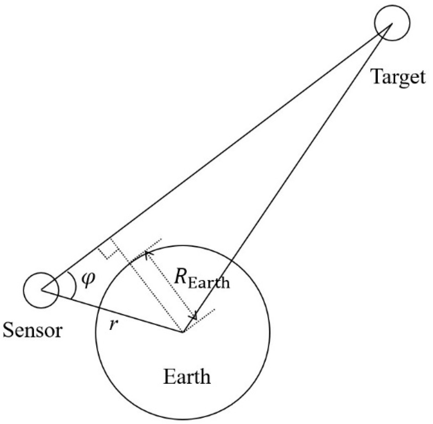
. The orbital data were simulated over the coming 48 h, with the line-of-sight not being blocked by the Earth as the visible condition. The specific judgment conditions are shown in
Figure 1. The target is blocked by the Earth when
and
. Here,
is the sensor orbit radius;
is the radius of the Earth; and
is the angle subtended by the Earth, the sensor, and the target. Then, 400 s continuous observation data were selected in different visible arc segments. The observation interval was 10 s, and the observation error was five arc seconds.
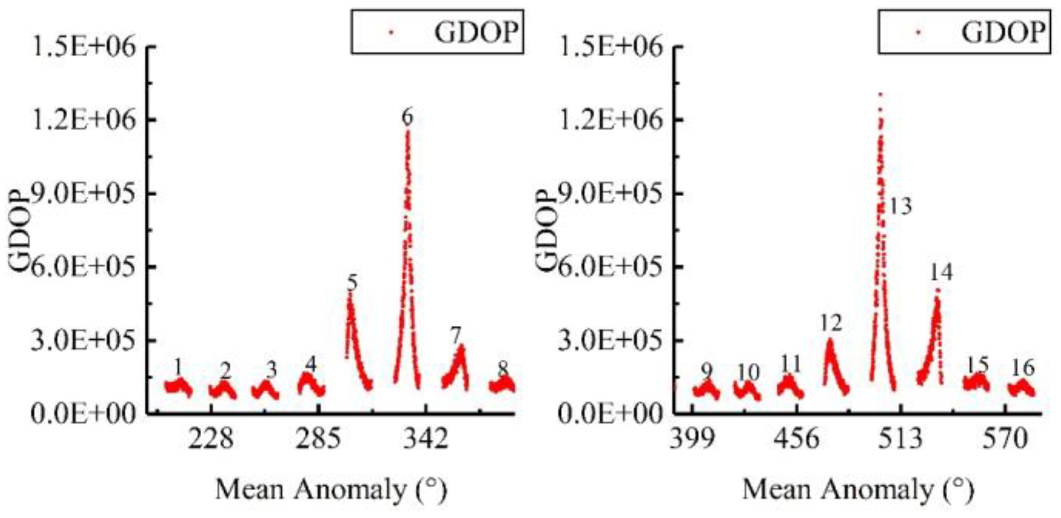
The GDOPs of different observable arc segments obtained through simulations using Equation (10) are shown in
Figure 2. Monte Carlo simulations were performed 100 times under each observation condition, following which, the covariance matrix and the GDOP were calculated. The results of the simulation experiment are shown in
Figure 3. It is worth noting that the situation of the UVM’s iterative process not converging occurred in the simulation experiments. If the iterative process of the UVM does not converge, the data are discarded. The iterative process is very complex. Dichter [
20] characterized the convergence behaviours of the orbit determination algorithm applied to the three angles-only data. There is no perfect method to determine whether UVM applied to multiple angles-only data converges so far.
As shown in
Figure 2, it is reasonable to calculate the GDOP using the analytic form of the target state obtained by assuming that the values of
,
, and
under short-arc conditions are constant. It can also be seen that the orbit determination accuracy varies periodically at different visible arc segments when observing the same target continuously. The period is approximately the orbital period of the optical sensor located in a lower orbit.
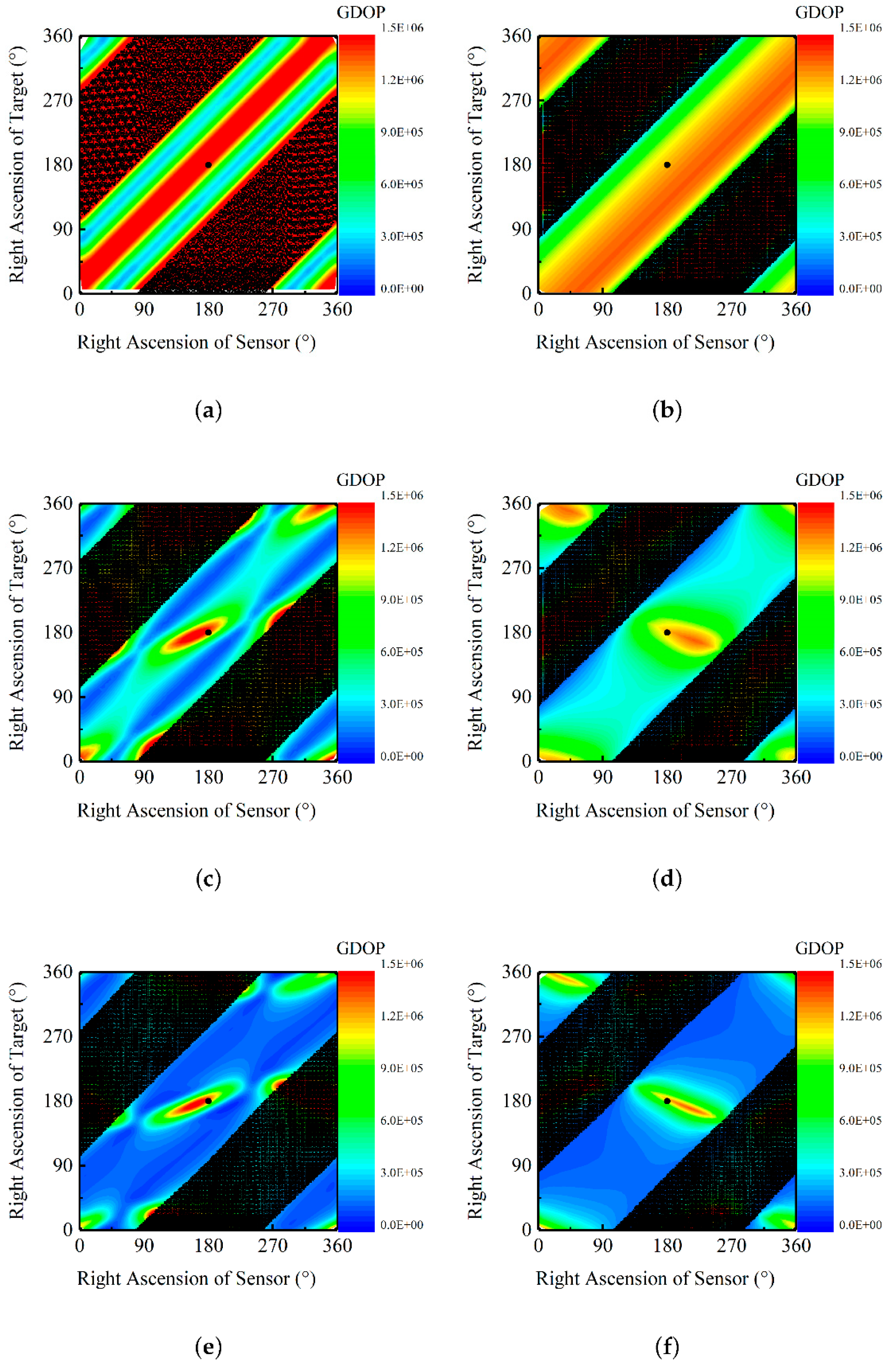
5.2. Effect of the Observation Geometry on GDOP
The radii of the optical sensor and target in the simulation experiment were
and
, respectively. The observation interval was 10 s, the observation arc length was 400 s, and the observation error was 5 arc seconds. The GDOPs corresponding to
and
were simulated as the starting observation times at different values of
. This corresponds to the accuracy of the initial orbit determination for all possible observation geometries under the specified radius of the target and optical sensor. It can be used to express the effect of the observation geometry on initial orbit determination. The simulation results are shown in
Figure 4.
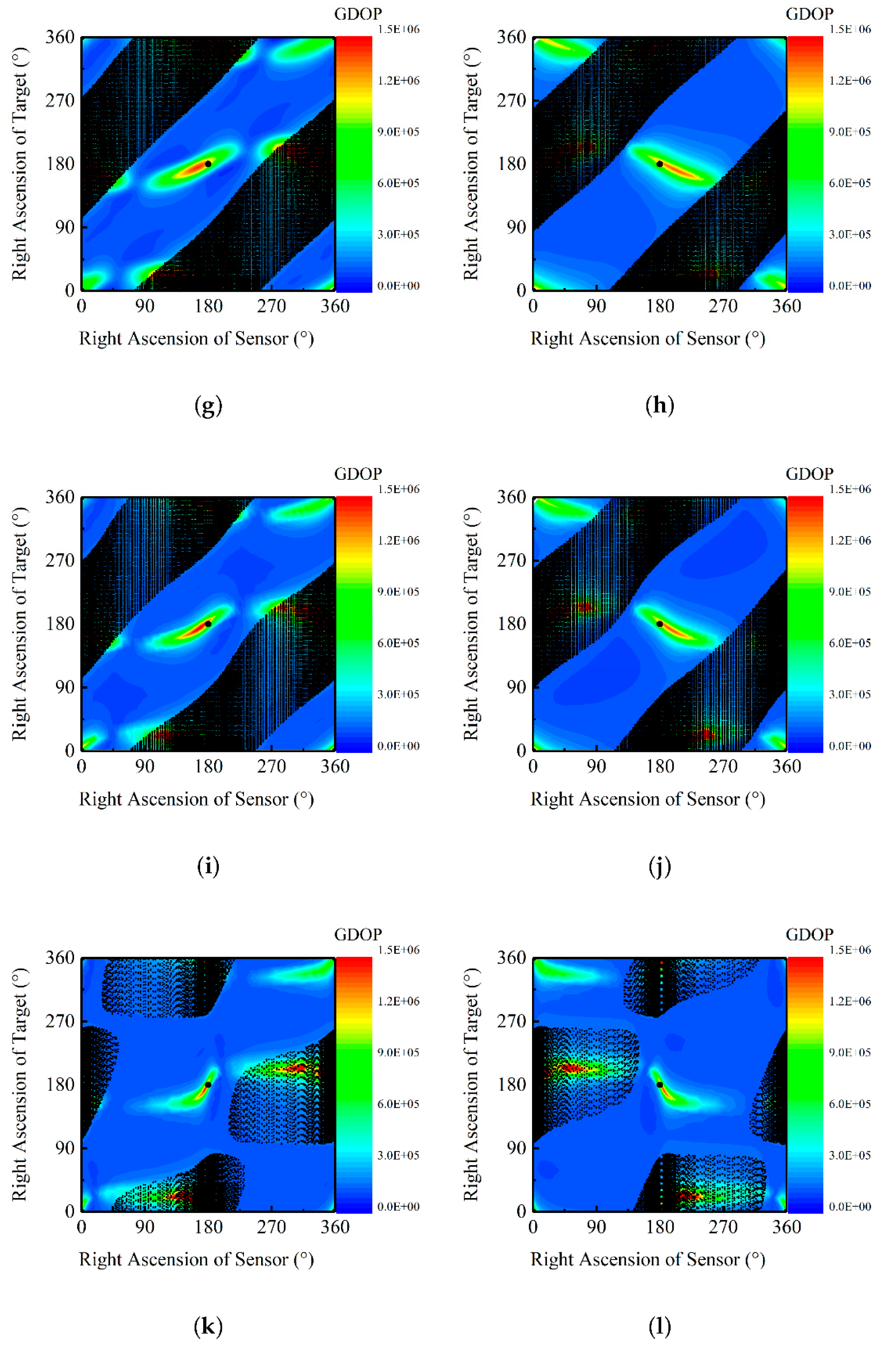
The shaded area in
Figure 4 indicates regions that are not visible. The simulation results are consistent with the conclusion that the initial orbit determination accuracy is poor when the target and optical sensor orbit planes are coplanar. The variation characteristics of GDOP with the right ascension of the target and the optical sensor are similar when the angles between the orbital planes of the target and the optical sensor are the same. However, owing to the different directions of the target and optical sensor motion, there are some differences in the GDOP for the same angle between orbital planes. Further, the GDOP is significantly larger when the right ascensions of the target and the optical sensor are close to
,
. The declination of the optical sensor is 0 when the right ascension of the optical sensor is 0°, 180° and 360°. At these times, the right ascension and declination of the target and the optical sensor are the same; the right ascension and declination of the target and the optical sensor in the natural coordinate system are also the same. It is important to note that, if we do not consider Earth blocking, it can be summarized that the GDOP is significantly larger when the target and the optical sensor are both close to the orbital plane intersection line than the other situations. The values of GDOP differ by more than 10 times. The actual calculation of the initial orbit with a large GDOP often results in iterative divergence. In other words, the optical sensor has the worst surveillance capability for targets in the same orbital plane or those nearly directly above it.
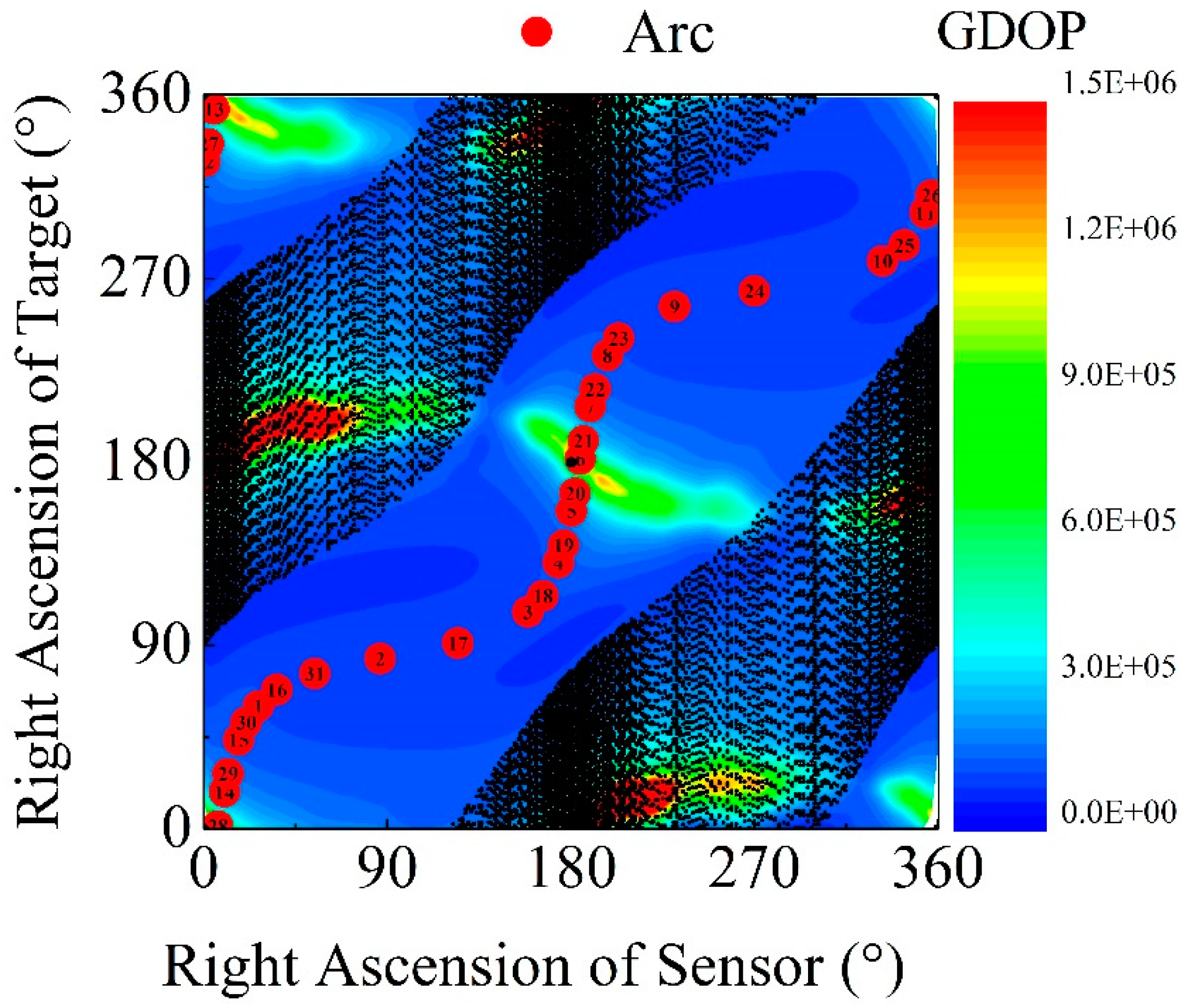
In the simulation experiment in
Section 5.1, the angle between the target and the optical sensor orbital plane was approximately 114.6°. Then, 400 s visible arcs were taken at the midpoint of each visible arc. The right ascension of the target and the optical sensor at the beginning of each observation arc segment are shown in
Figure 5. The arcs 6, 13, 20, 21, and 28—with large GDOPs—correspond to scenarios where the target and the optical sensor are close to the same right ascension and declination.
6. Discussion
This study analyses the effect of the observation geometry on the short-arc angles-only initial orbit determination, finding that the optical sensor has the worst surveillance capability for targets in the same orbital plane or those nearly directly above it.
First, the GDOP is chosen to describe the accuracy of initial orbit determination. The specific form of the GDOP is derived using the UVM, which is the linear orbit determination equation for the target state. Simulation experiments show that the approximate Lagrangian coefficients and distances are constant for short observation arcs and have little effect on the covariance matrix. At this point, the GDOP is close to the analytical form. Then, a method is proposed to represent all possible observation geometries in terms of the right ascension of the target and optical sensor, along with the angle between the target and optical sensor orbital planes in a new coordinate system. Through simulation experiments, it is concluded that the accuracy of the initial orbit determination is poor in two cases for all conditions—when the target and sensor are at the same right ascension and declination or when the orbital planes of the target and sensor are close to coplanarity.
This article focuses on the influence of the observation geometry on the initial orbit determination algorithm from a computational point of view. The observation error was assumed to be constant in the simulation experiment. The observation conditions of the target are influenced by the observation geometry and the position of the sun. Observation errors may vary for the same optical sensor with different observation geometries. The observation error and GDOP are approximately linearly related. The effect of the Sun’s relative position on the observation error can be added as an additional factor to the conclusions of this paper.


