
An Improved Point Cloud Upsampling Algorithm for X-ray Diffraction on Thermal Coatings of Aeroengine Blades

 ,
,
Abstract
:1. Introduction
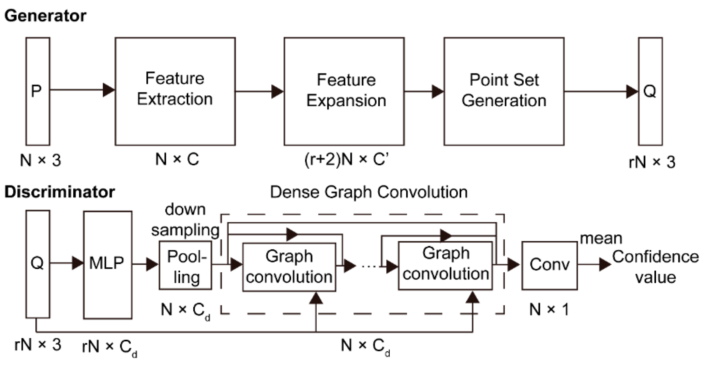
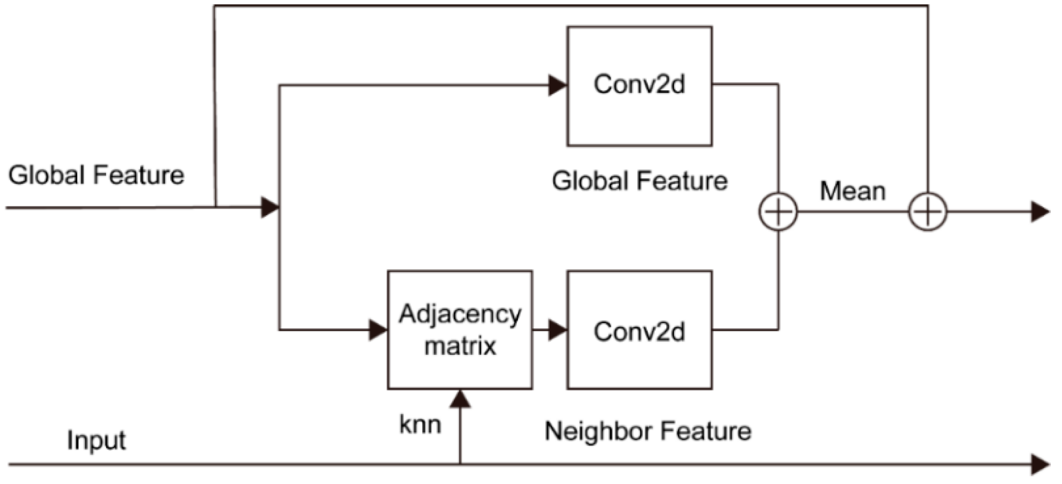
2. Methodology
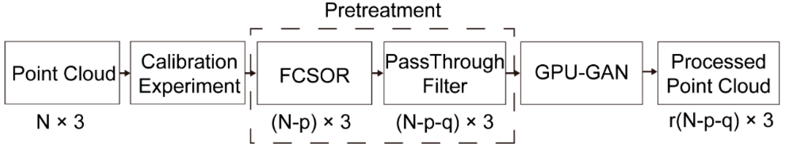
| Algorithm 1 Pretreatment |
| Input: Point cloud |
| Output: Filtered point cloud |
| 1: function Fast cluster statistic outlier removal () 2: Defining cluster size 3: 4: |
| 5: |
| 6: |
| 7: Subdividing point cloud space into N clusters 8: for do 9: |
| 10: add appropriate cluster 11: end for |
| 12: 13: Retain clusters with number of points less than 14: for do 15: 16: 17: 18: end for 19: return 20: end function 21: |
| 22: function Pass-through filter () 23: Defining experimental area (EA) 24: 25: 26: 27: 28: return |
| 29: end function |
3. Experiments
3.1. Data and Implementation Details
3.2. Evaluation Metrics
3.3. Analysis and Comparison of Experimental Results
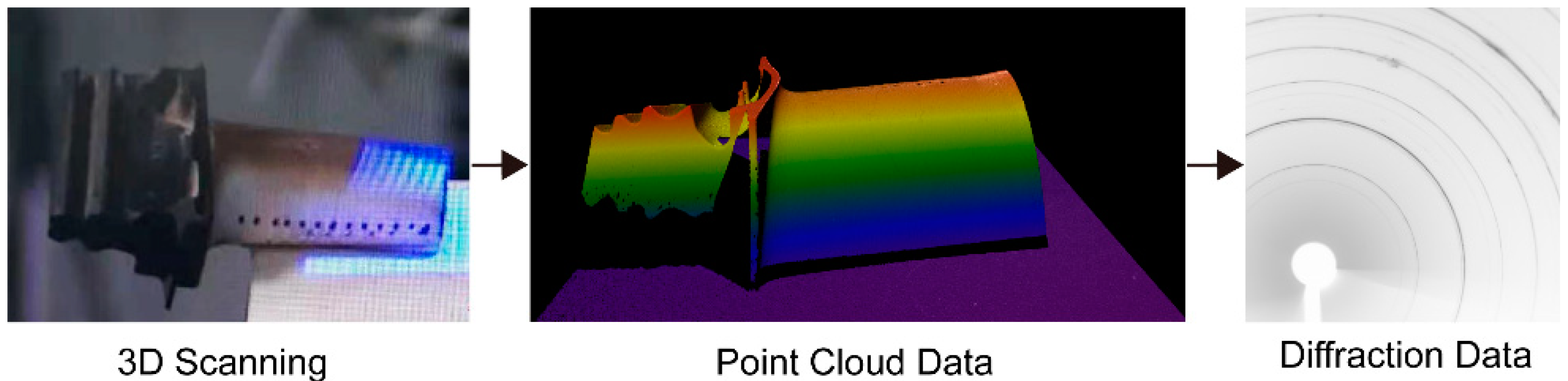
3.4. X-ray Diffraction Experiment
4. Conclusions
Author Contributions
Funding
Data Availability Statement
Acknowledgments
Conflicts of Interest
References
- Padture, N.P.; Gell, M.; Jordan, E.H.J.S. Thermal barrier coatings for gas-turbine engine applications. Science 2002, 296, 280–284. [Google Scholar] [CrossRef]
- Schulz, U.; Leyens, C.; Fritscher, K.; Peters, M.; Saruhan-Brings, B.; Lavigne, O.; Dorvaux, J.-M.; Poulain, M.; Mévrel, R.; Caliez, M.J.A.S.; et al. Some recent trends in research and technology of advanced thermal barrier coatings. Aerosp. Sci. Technol. 2003, 7, 73–80. [Google Scholar] [CrossRef]
- Drakopoulos, M.; Connolley, T.; Reinhard, C.; Atwood, R.; Magdysyuk, O.; Vo, N.; Hart, M.; Connor, L.; Humphreys, B.; Howell, G. I12: The joint engineering, environment and processing (JEEP) beamline at diamond light source. J. Synchrotron Radiat. 2015, 22, 828–838. [Google Scholar] [CrossRef] [PubMed]
- Siddiqui, S.F.; Knipe, K.; Manero, A.; Meid, C.; Wischek, J.; Okasinski, J.; Almer, J.; Karlsson, A.M.; Bartsch, M.; Raghavan, S.J.R.o.S.I. Synchrotron X-ray measurement techniques for thermal barrier coated cylindrical samples under thermal gradients. Rev. Sci. Instrum. 2013, 84, 083904. [Google Scholar] [CrossRef] [PubMed] [Green Version]
- Tie-Ying, Y.; Wen, W.; Guang-Zhi, Y.; Xiao-Long, L.; Mei, G.; Yue-Liang, G.; Li, L.; Yi, L.; He, L.; Xing-Min, Z. Introduction of the X-ray diffraction beamline of SSRF. Nucl. Sci. Tech. 2015, 26, 20101-020101. [Google Scholar] [CrossRef]
- Charles, R.Q.; Su, H.; Kaichun, M.; Guibas, L.J. PointNet: Deep Learning on Point Sets for 3D Classification and Segmentation. In Proceedings of the 2017 IEEE Conference on Computer Vision and Pattern Recognition (CVPR), Honolulu, HI, USA, 21–26 July 2017; pp. 77–85. [Google Scholar] [CrossRef] [Green Version]
- Qi, C.R.; Yi, L.; Su, H.; Guibas, L.J. Pointnet++: Deep hierarchical feature learning on point sets in a metric space. In Proceedings of the Advances in Neural Information Processing Systems, Long Beach, CA, USA, 4–9 December 2017; pp. 5105–5114. [Google Scholar]
- Wang, Y.; Sun, Y.; Liu, Z.; Sarma, S.E.; Bronstein, M.M.; Solomon, J.M. Dynamic graph cnn for learning on point clouds. Acm Trans. Graph. 2019, 38, 1–12. [Google Scholar] [CrossRef] [Green Version]
- Yu, L.; Li, X.; Fu, C.-W.; Cohen-Or, D.; Heng, P.-A. Pu-net: Point cloud upsampling network. In Proceedings of the IEEE Conference on Computer Vision and Pattern Recognition, Salt Lake City, UT, USA, 18–23 June 2018; pp. 2790–2799. [Google Scholar] [CrossRef] [Green Version]
- Yu, L.; Li, X.; Fu, C.-W.; Cohen-Or, D.; Heng, P.-A. Ec-net: An edge-aware point set consolidation network. In Proceedings of the European Conference on Computer Vision (ECCV), Munich, Germany, 8–14 September 2018; pp. 386–402. [Google Scholar] [CrossRef] [Green Version]
- Yifan, W.; Wu, S.; Huang, H.; Cohen-Or, D.; Sorkine-Hornung, O. Patch-based progressive 3d point set upsampling. In Proceedings of the IEEE/CVF Conference on Computer Vision and Pattern Recognition, Long Beach, CA, USA, 15–20 June 2019; pp. 5958–5967. [Google Scholar] [CrossRef] [Green Version]
- Qian, G.; Abualshour, A.; Li, G.; Thabet, A.; Ghanem, B. PU-GCN: Point Cloud Upsampling using Graph Convolutional Networks. In Proceedings of the IEEE/CVF Conference on Computer Vision and Pattern Recognition, Long Beach, CA, USA, 15–20 June 2019. [Google Scholar] [CrossRef]
- Li, R.; Li, X.; Fu, C.-W.; Cohen-Or, D.; Heng, P.-A. Pu-gan: A point cloud upsampling adversarial network. In Proceedings of the IEEE/CVF International Conference on Computer Vision, Seoul, Korea, 27 October–2 November 2019; pp. 7203–7212. [Google Scholar] [CrossRef] [Green Version]
- Rusu, R.B.; Marton, Z.C.; Blodow, N.; Dolha, M.; Beetz, M. Towards 3D point cloud based object maps for household environments. Robot. Auton. Syst. 2008, 56, 927–941. [Google Scholar] [CrossRef]
- Miknis, M.; Davies, R.; Plassmann, P.; Ware, A. Near real-time point cloud processing using the PCL. In Proceedings of the 2015 International Conference on Systems, Signals and Image Processing (IWSSIP), Singapore, 10–12 September 2015; pp. 153–156. [Google Scholar] [CrossRef]
- Balta, H.; Velagic, J.; Bosschaerts, W.; De Cubber, G.; Siciliano, B. Fast statistical outlier removal based method for large 3D point clouds of outdoor environments. IFAC-PapersOnLine 2018, 51, 348–353. [Google Scholar] [CrossRef]
- Wu, H.; Zhang, J.; Huang, K. Point cloud super resolution with adversarial residual graph networks. arXiv Prepr. 2019, arXiv:02111. [Google Scholar] [CrossRef]
- He, K.; Zhang, X.; Ren, S.; Sun, J. Deep residual learning for image recognition. In Proceedings of the 2016 IEEE Conference on Computer Vision and Pattern Recognition (CVPR), Las Vegas, NV, USA, 27–30 June 2016; pp. 770–778. [Google Scholar] [CrossRef] [Green Version]
- Huang, G.; Liu, Z.; Van Der Maaten, L.; Weinberger, K.Q. Densely connected convolutional networks. In Proceedings of the 2017 IEEE Conference on Computer Vision and Pattern Recognition, Honolulu, HI, USA, 21–26 July 2017; pp. 2261–2269. [Google Scholar] [CrossRef] [Green Version]
- Fan, H.; Su, H.; Guibas, L.J. A point set generation network for 3d object reconstruction from a single image. In Proceedings of the IEEE Conference on Computer Vision and Pattern Recognition, London, UK, 21–26 July 2017; pp. 605–613. [Google Scholar] [CrossRef] [Green Version]
- Kingma, D.P.; Ba, J. Adam: A method for stochastic optimization. arXiv Prepr. 2014, arXiv:1412.6980. [Google Scholar] [CrossRef]
- Heusel, M.; Ramsauer, H.; Unterthiner, T.; Nessler, B.; Hochreiter, S. Gans trained by a two time-scale update rule converge to a local nash equilibrium. In Proceedings of the Advances in Neural Information Processing Systems, Long Beach, CA, USA, 4–9 December 2017; pp. 6629–6640. [Google Scholar]
- Abadi, M.; Barham, P.; Chen, J.; Chen, Z.; Davis, A.; Dean, J.; Devin, M.; Ghemawat, S.; Irving, G.; Isard, M. {TensorFlow}: A System for {Large-Scale} Machine Learning. In Proceedings of the 12th USENIX Symposium on Operating Systems Design and Implementation (OSDI 16), Savannah, GA, USA, 2–4 November 2016; pp. 265–283. [Google Scholar]
- Rusu, R.B.; Cousins, S. 3d is here: Point cloud library (pcl). In Proceedings of the 2011 IEEE International Conference on Robotics and Automation, Shanghai, China, 9–13 May 2011; pp. 1–4. [Google Scholar] [CrossRef] [Green Version]
- Cignoni, P.; Callieri, M.; Corsini, M.; Dellepiane, M.; Ganovelli, F.; Ranzuglia, G. Meshlab: An open-source mesh processing tool. In Proceedings of the Eurographics Italian Chapter Conference, Salerno, Italy, 2–4 July 2008; pp. 129–136. [Google Scholar] [CrossRef]


| Method | CD | EMD | F-Score | NUC with Different p | Deviation | Time | |||||
|---|---|---|---|---|---|---|---|---|---|---|---|
| τ = 0.01 | τ = 0.02 | 0.2% | 0.4% | 0.6% | mean | std | Trian (h) | Test (min) | |||
| MPU | 0.026 | 0.888 | 0.091 | 0.495 | 19.087 | 10.807 | 8.225 | 0.021 | 0.068 | 15.7 | 42.1 |
| PU-GAN | 0.032 | 1.357 | 0.258 | 0.564 | 17.967 | 9.641 | 6.753 | 0.018 | 0.017 | 19.2 | 55.6 |
| GPU-GAN | 0.024 | 1.126 | 0.328 | 0.649 | 17.855 | 9.505 | 6.522 | 0.016 | 0.023 | 21.1 | 56.3 |
| Filter + MPU | 0.016 | 0.362 | 0.106 | 0.583 | 13.201 | 9.869 | 5.772 | 0.019 | 0.009 | - | 29.3 |
| Filter + PU-GAN | 0.016 | 0.447 | 0.293 | 0.654 | 12.317 | 8.909 | 4.845 | 0.016 | 0.009 | - | 38.5 |
| Filter + GPU-GAN | 0.014 | 0.405 | 0.375 | 0.753 | 12.295 | 8.866 | 4.792 | 0.014 | 0.008 | - | 38.9 |
Publisher’s Note: MDPI stays neutral with regard to jurisdictional claims in published maps and institutional affiliations. |
© 2022 by the authors. Licensee MDPI, Basel, Switzerland. This article is an open access article distributed under the terms and conditions of the Creative Commons Attribution (CC BY) license (https://creativecommons.org/licenses/by/4.0/).
Share and Cite
Zhao, W.; Wen, W.; Liu, K.; Zhang, Y.; Wang, Q.; Yin, G.; Sun, B.; Zhang, Y.; Gao, X. An Improved Point Cloud Upsampling Algorithm for X-ray Diffraction on Thermal Coatings of Aeroengine Blades. Appl. Sci. 2022, 12, 6807. https://doi.org/10.3390/app12136807
Zhao W, Wen W, Liu K, Zhang Y, Wang Q, Yin G, Sun B, Zhang Y, Gao X. An Improved Point Cloud Upsampling Algorithm for X-ray Diffraction on Thermal Coatings of Aeroengine Blades. Applied Sciences. 2022; 12(13):6807. https://doi.org/10.3390/app12136807
Chicago/Turabian StyleZhao, Wenhan, Wen Wen, Ke Liu, Yan Zhang, Qisheng Wang, Guangzhi Yin, Bo Sun, Ying Zhang, and Xingyu Gao. 2022. "An Improved Point Cloud Upsampling Algorithm for X-ray Diffraction on Thermal Coatings of Aeroengine Blades" Applied Sciences 12, no. 13: 6807. https://doi.org/10.3390/app12136807