Article

Automatic False Alarm Detection Based on XAI and Reliability Analysis

Department of Information Security, Hoseo University, Asan 31499, Korea
*
Author to whom correspondence should be addressed.
Appl. Sci. 2022, 12(13), 6761; https://doi.org/10.3390/app12136761
Submission received: 14 June 2022 / Revised: 29 June 2022 / Accepted: 30 June 2022 / Published: 4 July 2022
(This article belongs to the Special Issue Recent Advances in Cybersecurity and Computer Networks)

Abstract

:
Many studies attempt to apply artificial intelligence (AI) to cyber security to effectively cope with the increasing number of cyber threats. However, there is a black box problem such that it is difficult to understand the basis for AI prediction. False alarms for malware or cyberattacks can cause serious side effects. Due to this limitation, all AI predictions must be confirmed by an expert, which is a considerable obstacle to AI expansion. Compared to the increasing number of cyberattack alerts, the number of alerts that can be analyzed by experts is limited. This paper provides explainability through an interpretation of AI prediction results and a reliability analysis of AI predictions based on explainable artificial intelligence (XAI). In addition, we propose a method for screening high-quality data that can efficiently detect false predictions based on reliability indicators. Through this, even a small security team can quickly respond to false predictions. To validate the proposed method, experiments were conducted using the IDS dataset and the malware dataset. AI errors were detected better than they could be by the existing AI models, with about 262% in the IDS dataset and 127% in the malware dataset from the top 10% of analysis targets. Therefore, the ability to respond to cyberattacks can be improved using the proposed method.

1. Introduction

Due to the development of IT infrastructure, network traffic has increased exponentially, and the number of users has also increased significantly. This has led to an increase in cyber security events. The number of cyber threats detected in 2020 increased by 12% from the previous year according to the McAfee Labs Threats Report published in November 2020 [1]. In 2021, there was a 50% increase in the overall attacks per week on corporate networks compared to in 2020 [2]. To solve this problem, various studies are underway to introduce machine learning and artificial intelligence (AI) technology that detects cyberattacks in an actual security environment. However, AI models often have high false positives due to the wide range of cyber threats. It is important to be able to trust AI predictions, but it is very difficult to understand the model due to the black-box nature of AI models. In high-risk and high-value-added industries such as energy, medical care, and finance, AI predictions are subject to too much risk to place trust in it without an explanation.
No matter how high the accuracy of AI, the additional analysis of an AI prediction by experts is inevitable. Therefore, accurate analysis is required for the security environment, so human analysts must directly intervene to respond to threats. There is a limit to preparing for the increasing security threats with security personnel alone.
One of the concerns in the current security landscape is that cyber threats are evolving rapidly and causing significant damage, but solutions are lacking. False detection applications in a security operation center (SOC) use predefined signatures to identify attacks. The signature database must be updated constantly, which is problematic in that it depends on user input. Additionally, the signature method is effective against known threats but ineffective against unknown threats. Under these limitations, the adoption of AI models has gradually increased, but these models suffer from a lack of reliability due to a high frequency of false detections. Therefore, system administrators are often forced to analyze the data themselves. Explainable artificial intelligence (XAI) analysis methods are being studied to explain the contribution of each feature to AI prediction based on perturbation or propagation. However, only interpretation according to feature contribution is possible, and it has not developed into a framework for the efficient analysis that is currently required [3,4,5]. Ultimately, human analysts will have to judge AI predictions themselves by analyzing the information obtained from the data. Unfortunately, according to a survey, 27% of the SOC’s of organizations receive more than 1 million security alerts daily, and while it is virtually impossible to respond to such an astronomical number, separating actual threats from false-positive alerts is also a crucial problem [6]. This problem occurs not only in NIDS environments but also in all security environments, such as in malware detection.
In this study, we propose a method for screening suspicious AI judgments with high analysis priority in order to analyze efficient attack alarms from limited human resources. The proposed method selects features that have contributed significantly to AI judgment through XAI and then measures the label bias of the data based on important features. Using the measured label bias and the degree of anomaly in the data, the proposed method measures the reliability of the AI judgment to provide an environment in which suspicious AI judgment can be analyzed first. In order to shorten the analysis time for the analyst, it is possible to display suspicious judgment data along with information that humans can understand. It is expected that productivity would be greatly improved if an expert’s analysis proceeds based on a reliability indicator and explainable information obtained through the proposed method.
The composition of this paper is as follows: The next section describes machine learning and XAI-related studies. Section 3 proposes a framework for providing trust indicators for the XAI-based AI models proposed in this paper. Section 4 describes the processes and results of experiments using the IDS dataset and the malware dataset to validate the proposed framework. Section 5 presents the discussion. Finally, Section 6 presents the conclusions.

2. Related Work

2.1. AI Cyber Threat Detection

With the advancement of technology, Internet usage is increasing, and cyberattacks are also increasing. Most cyberattacks can be detected based on signatures, but unknown attacks are difficult to detect. To solve this problem, various AI technologies are being applied, and through this, cyberattacks such as malware and intrusion can be detected [7,8]. Venkatraman et al. proposed a new, integrated hybrid deep learning and visualization approach for effective malware detection and experimentally calculated high classification accuracy to verify the performance of the proposed framework [9]. Ding et al. proposed training an IDS model based on convolution neural networks (CNN), a typical deep learning method, using an IDS dataset [10]. A security expert should form an appropriate response depending on the analysis results of the events that have occurred, the logs, and the detection system. A wrong judgment can cause serious damage, so it is necessary to accurately distinguish between what is normal and what is an attack. However, there are many cases when the AI detection system is actually normal but predicts an attack (FN), or when there is actually an attack that is predicted to be normal (FP). There are two ways to respond to false alarms. The first is a method that reduces false alarms by increasing the accuracy of the model itself, while the second fine-tunes the post-processing of false alarms. Improving the performance of the model is difficult; furthermore, even if the performance improvement is successful and the accuracy is high, the performance may be inadequate to detect cyberattacks that feature future technological advances and evolving attack strategies. Therefore, it is better to improve the quality of false alarms through post-processing. There are studies that have succeeded in processing an alarm set based on the distribution of false alarms [11,12]. Although the rate of false alarms in the overall alarm set has decreased, it can be seen that the number of true alarms has also decreased [13].

2.2. XAI

AI technology can process a large amount of work in real-time, but it is difficult for users to trust it because the basis of and process for the results cannot be known [14]. An interpretation of an AI model should make it possible to overcome this limitation. Research to analyze and improve the results derived through AI is actively being conducted [15]. Guidotti et al. explained the interpretability of black-box decision-making systems through various approaches [16]. This was based on the fact that a hidden internal system comprising a decision support system (DSS) plays an important role in making more useful decisions. DSS is a system that provides information by analyzing a large amount of data, which is critical in the era of big data. Amarasinghe and Manic conducted a study on a methodology for generating feedback to users regarding the decision-making process of deep neural networks—IDS [15].
In order to interpret the predictions of a model, XAI, which can explain model predictions, is being studied to improve the transparency of models [17]. The interpretation of a model can be evaluated from two perspectives, i.e., the possibility of interpretation and the transparency of the model [18]. If the explainer focuses on the transparency of the model, the explanation is difficult to understand from the user’s point of view because the focus is on the purpose for delivering accurate facts. An emphasis on interpretability provides explanations that can be more easily understood by the user, but many elements are excluded to aid in understanding, which makes the explanation less reliable. Therefore, selecting an explainer that fits the situation is also an important process in interpretation.
The AI Explainability 360 toolkit provides an explainer based on the descriptive classification method [18]. There is a What-If Tool, which is an open-source application that allows practitioners to probe, visualize, and analyze machine learning systems while using minimal coding [19]. Given that the analysis of AI models provides confidence in AI through XAI, the need for XAI is emphasized [20]. Users can justify a decision or action based on the explanation presented by the XAI explainer [21].
Shapley additive explanation (SHAP) is a model that can be explained using the SHAP value based on the importance of the feature [3]. In 2017, Lundberg and Lee developed a Python package that could calculate the SHAP for various technologies, including LightGBM, XGBoost, Gboost, CatBoost Scikit-learn, and tree models [22]. For the interpretation of AI models that are difficult to interpret, many researchers have begun using SHAP [23]. Wang et al. proposed a framework to provide regional and global explanations for IDS judgments [24]. The framework presented in the paper explains the reason for the judgment made by IDS as the average of the SHAP value, which is insufficient for analyzing the correlation between the feature and the SHAP value. Only an analysis of the relationship between attacks and features and overall analysis is possible. The limitation of this framework is that it cannot resolve the reliability issues of the AI model. Further, Kim et al. proposed a method for the automatic screening of valuable alerts based on XAI [25]. This study also proposes a method to detect critical alerts that need to be analyzed by humans in real security environments where many attack alerts occur. In Section 4, we compare the results of this paper using the same dataset.

3. Materials and Methods
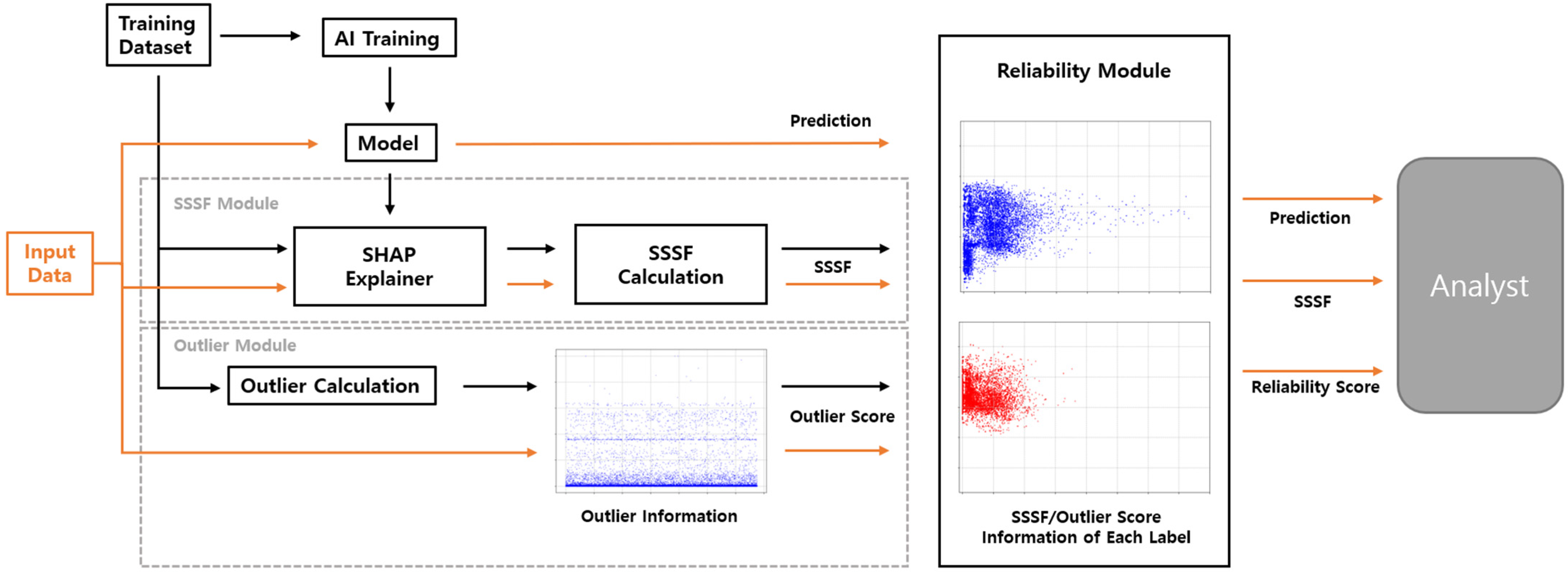
Currently, AI technology is being used to counter a flood of cyberattacks. However, AI models pose a risk of false predictions. There may be cases in which an attack is judged to be normal and allowed, or a normal event is judged to be an attack and is blocked. In order to minimize these errors, additional analysis is carried out by analysis experts in a real environment. However, it is impossible to analyze and respond to all of the countless attack alerts. To compensate for this, in this study, we propose a method for measuring alerts that are highly likely to be false predictions, which should be analyzed by experts in a real environment where many attack alerts occur. In addition, because the proposed method is based on explaining the prediction basis of the AI model, it is possible to provide useful information to the analyst.

3.1. Overview

We can learn the features that are important for the AI model to predict, and based on this, we can measure the reliability of the AI model prediction. The reliability of the AI model has two aspects—the analyst and AI—for calculating the two indicators. A composition diagram of the proposed method is as shown in Figure 1. After we train the AI model with the training dataset, we make a summary plot for each label using the SHAP explainer. The summary plot of each label can be easily compared and identified for each feature by the degree of that SHAP value’s contribution to prediction with the corresponding label. We then select important features that substantially contribute to the prediction with each label. After that, the sum of the SHAP value of the selected feature (SSSF) is used as the first indicator. Here, using the outlier algorithm, the reliability score that additionally considers the outliers based on the feature values is measured and used as the second indicator. We used k-nearest neighbors (k-NN) as an outlier algorithm in the proposed method. SSSF is an indicator of the degree to which the data are biased toward the label based on important features from the human point of view, and the reliability score is an indicator that adds the outlier score, which is a minute difference in the data that the model sees from the AI point of view. Through these two indicators, we propose a method for screening important alerts for subsequent analysis in a real security environment where many threats occur.

3.2. Preparing for Analysis

We learn the AI model after preprocessing the raw dataset so that it is suitable for learning. After that, two tasks must proceed to generate the indicators. First, it is necessary to select important features. Second, we generate an outlier calculation module.
SHAP is an algorithm that measures the contribution of each feature to the prediction when an AI model predicts data. SHAP uses the SHAP value as a basis for explanation. The SHAP value is a sampling value that measures the degree of influence through the extracted SHAP value. The formula for extracting the SHAP value is as follows:
ϕ i = S F \ j | S | ! ( | F | | S | 1 ) ! | F | ! [ f S   i ( x S   i ) f S ( x S ) ] ϕ i
where ϕi represents the SHAP value for the i-th instance; F represents the entire set; S represents all subsets except for the i-th instance in the entire set; f(Si)(x(Si)) represents the contribution that includes the i-th instance; and fS(xS) represents the contribution of the subset without the i-th data. The AI model trained on the training dataset calculates the SHAP value for the training dataset through the SHAP explainer. It is possible to check the extracted SHAP value of one instance through the force plot, as shown in Figure 2. The SHAP value of the feature called “DllCharacteristics” of the instance is 0.7872; thus, this feature can be interpreted as a feature that contributes to malware prediction.
After the algorithm calculates the SHAP value for each instance, the training dataset is classified by the label. We created a SHAP summary plot of the data corresponding to each label and selected important features based on the summary plot. Figure 3 shows the summary plot for predicting malware based on the malware dataset. The x-axis of the plot is the SHAP value of an instance, each point corresponds to an individual instance, and high and low feature values are represented in color. In Figure 3, “CheckSum” has the largest average SHAP value at the top, and it can be seen as the feature that contributes to the prediction the most. It can be interpreted that the blue instances distributed on the left have a negative effect on judging instances as malware because the feature value is small and the SHAP value is small, and it can be interpreted that the instances distributed on the right have a positive effect on judging instances as malware. Based on the distribution of these SHAP values, it is possible to explain the basis for the prediction of the AI model. A summary plot is used to select important features and to generate indicators. The criteria for the selection of important features are as follows. The contribution of the feature itself is ranked high, and the interpretation of the shape value distribution for each feature value should be clear. In addition, features have a positive effect on predicting using the label.
Next, an outlier calculation module is created. Outlier calculation refers to how far the data are from other data and how different they are. The outlier algorithm measures the degree of difference based on all feature values in the training dataset. It implies how far away the input data from the general trend of the training dataset are because AI can precisely determine minute differences that analysts cannot identify.

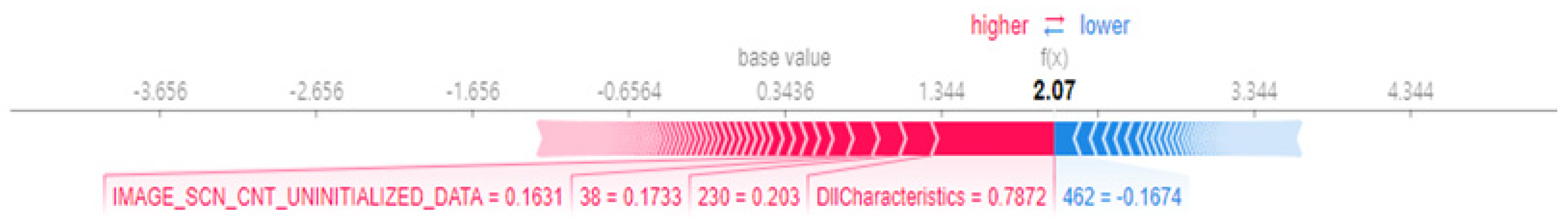
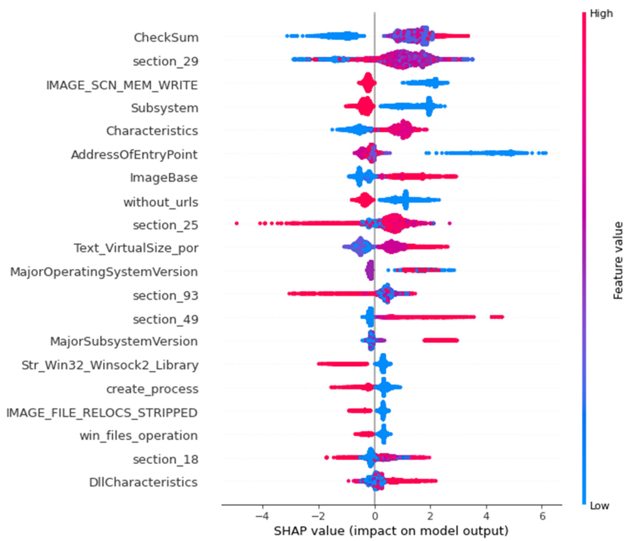
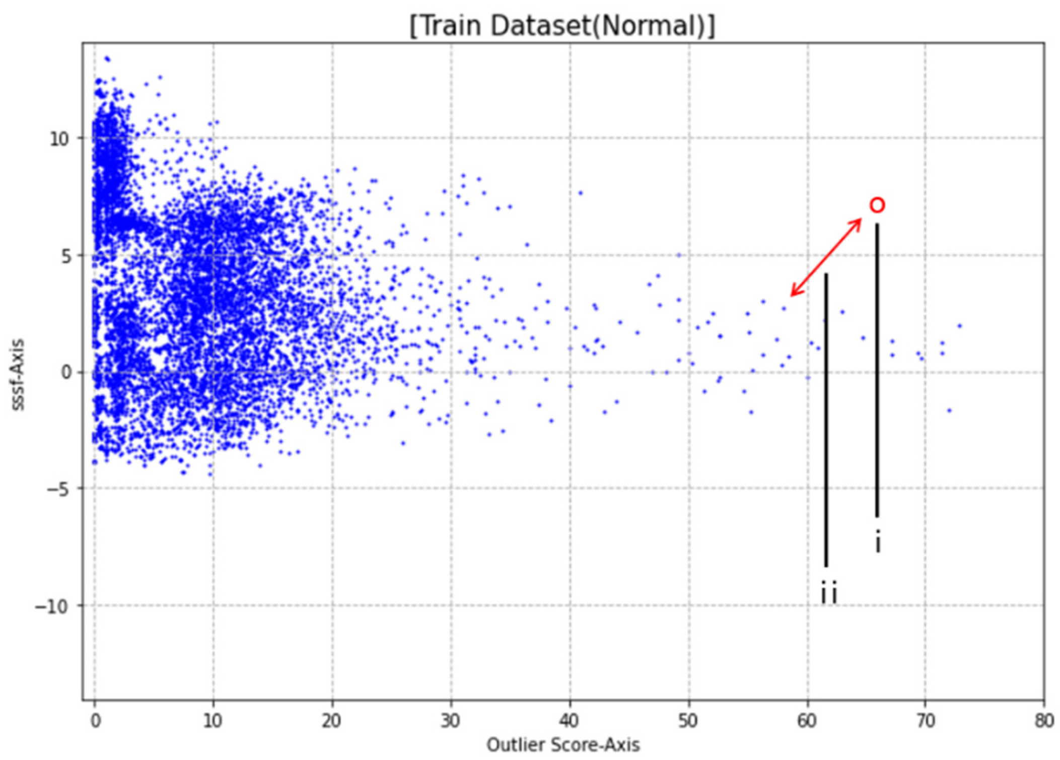
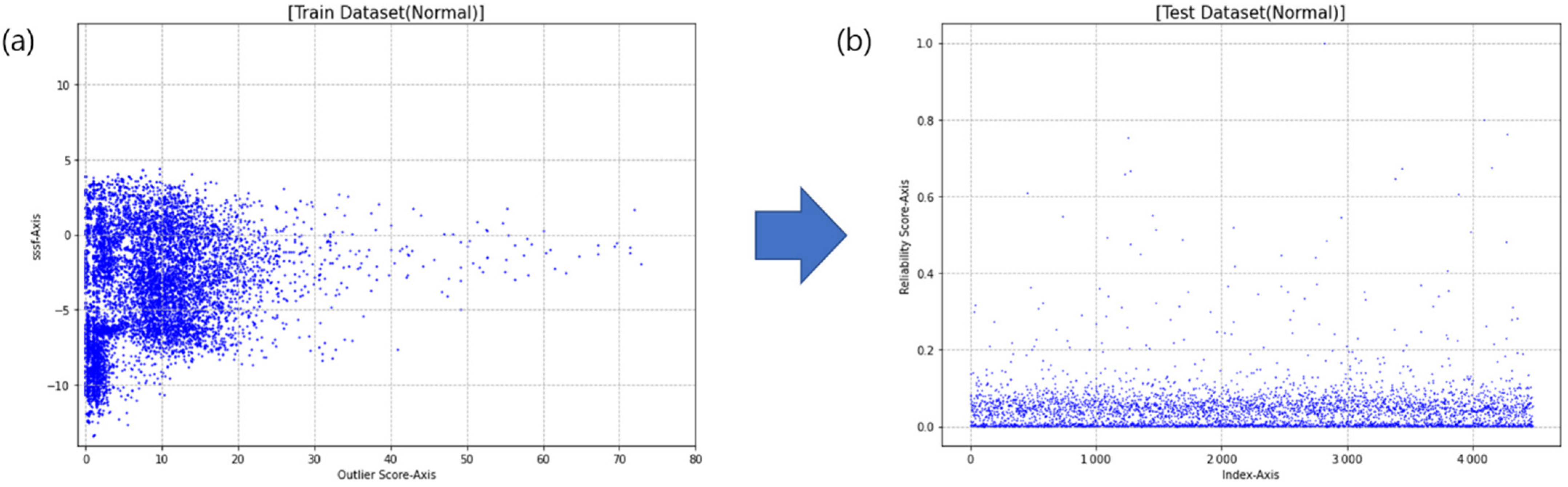
3.3. Reliability Analysis

Indicators are used to examine the parts that AI can predict incorrectly. SSSF is an indicator that can be interpreted intuitively from a human point of view, and here, the part that AI can predict incorrectly by representing the minute differences in data from an AI point of view is examined.
The SHAP value of a single feature provides information about how the feature value contributes to the prediction made by the AI model. The overall properties of the data can be inferred through complex features that represent data rather than a single feature. The features represented here are the important features that were previously selected. The sum of the SHAP value of the selected feature (SSSF) gathers the label tendency of each feature to reveal the overall label tendency of the data.
After we calculate the SSSF of the dataset, we classify the data by label and look at the SSSF distribution to understand the properties of the label. For data predicted to be malware, the SHAP value of the selected features will generally be high, and the SSSF will also naturally be high. For the data predicted by AI as normal, the SHAP value of the selected features will generally be low, and the SSSF will of course also come out low. It is possible to evaluate the reliability of the judgment by looking at the degree of difference from this expectation, and it is possible to interpret from a human point of view based on SHAP.
SSSF is an indicator of what AI judges incorrectly from a human point of view, whereas the reliability score is an indicator of what AI judges incorrectly by adding interpretable indicators that are intuitive from an AI point of view. The reliability score is calculated by measuring the degree of the anomaly of SSSF and the outlier score. Figure 4 briefly explains how the reliability score for the test data is calculated. After calculating the SSSF and outlier score of test data, which are new input data, the distance between the SSSF and outlier score of the training dataset is measured and used as a reliability score. It is calculated in the same way as the existing outlier score, but it is measured based on two-dimensional data consisting of SSSF and an outlier score and not based on all of the feature values. A reliability score that uses the outlier score along with the SSSF analyzes the general trend of the training dataset and means a degree of difference.

4. Experimental Results

We experimented using two datasets to verify the proposed method. The NSL-KDD [26], a public dataset for NIDS, and the 2019 KISA Data Challenge Dataset [27] for malware were used.

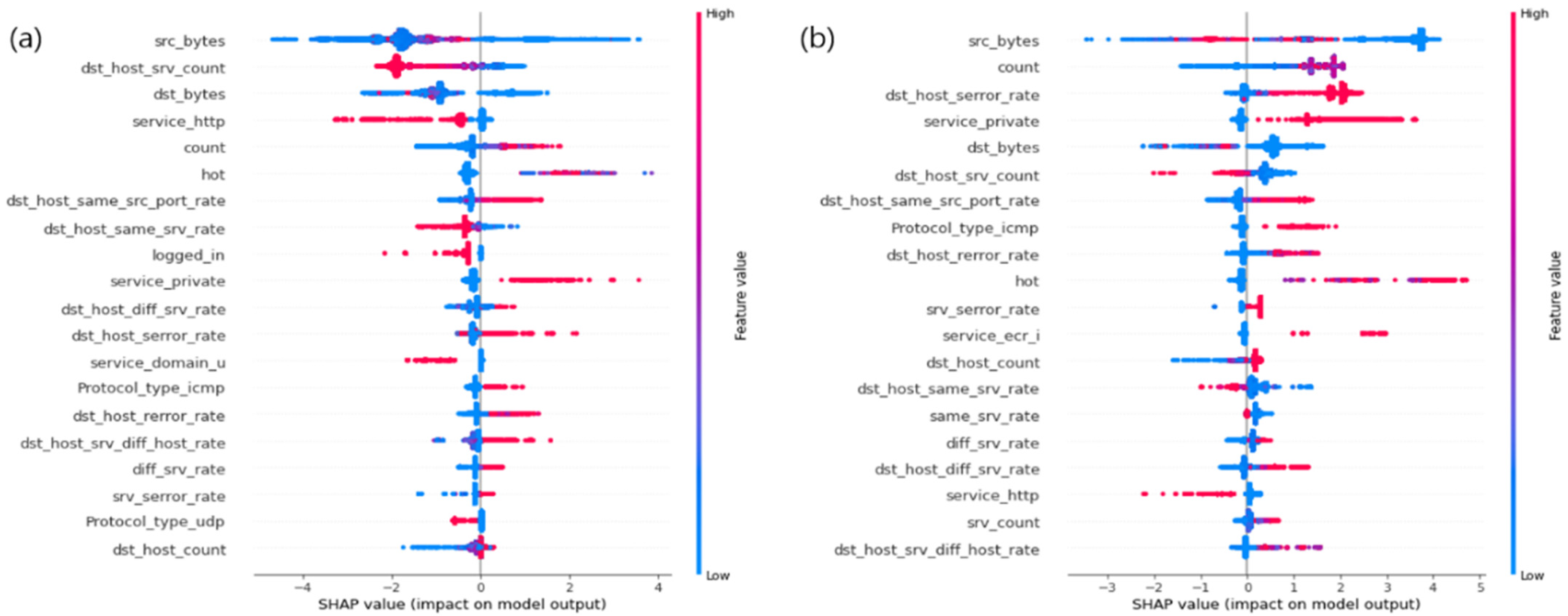
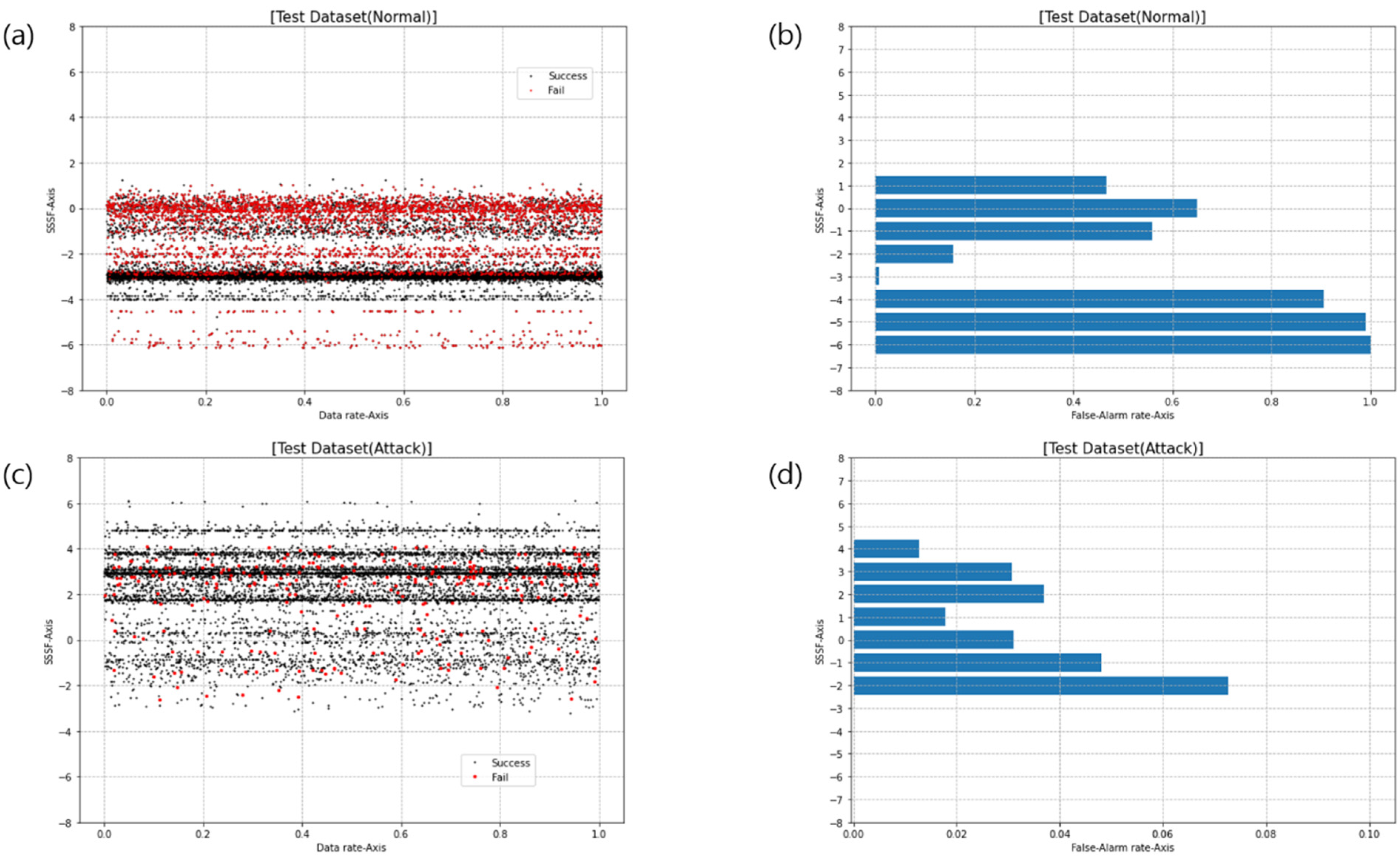
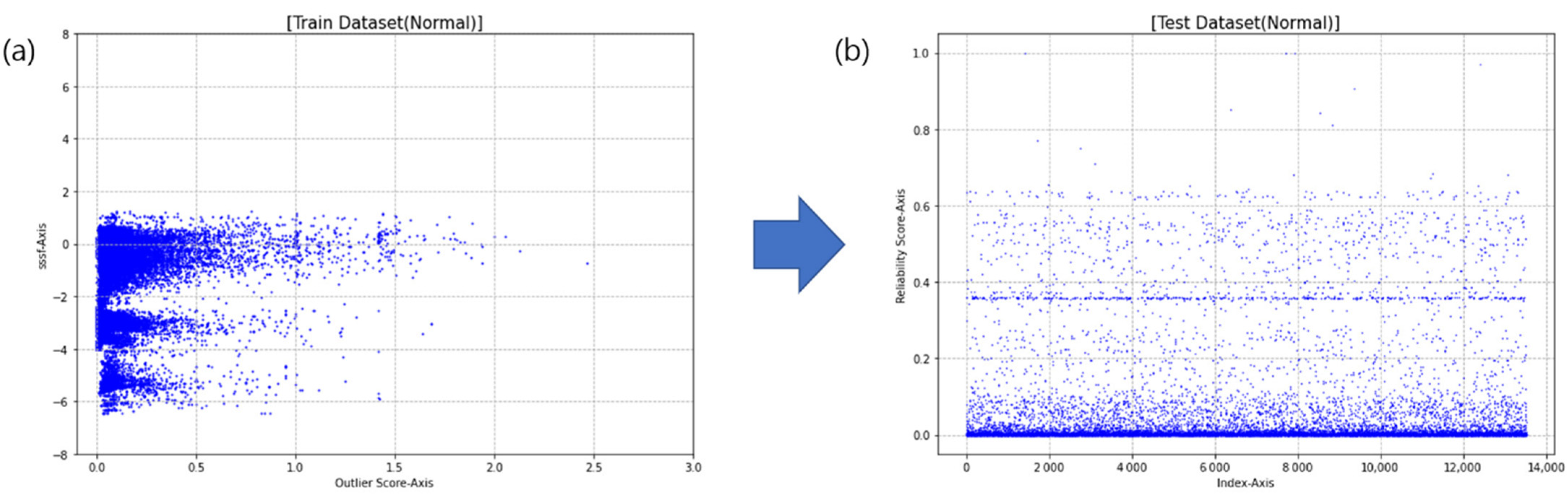
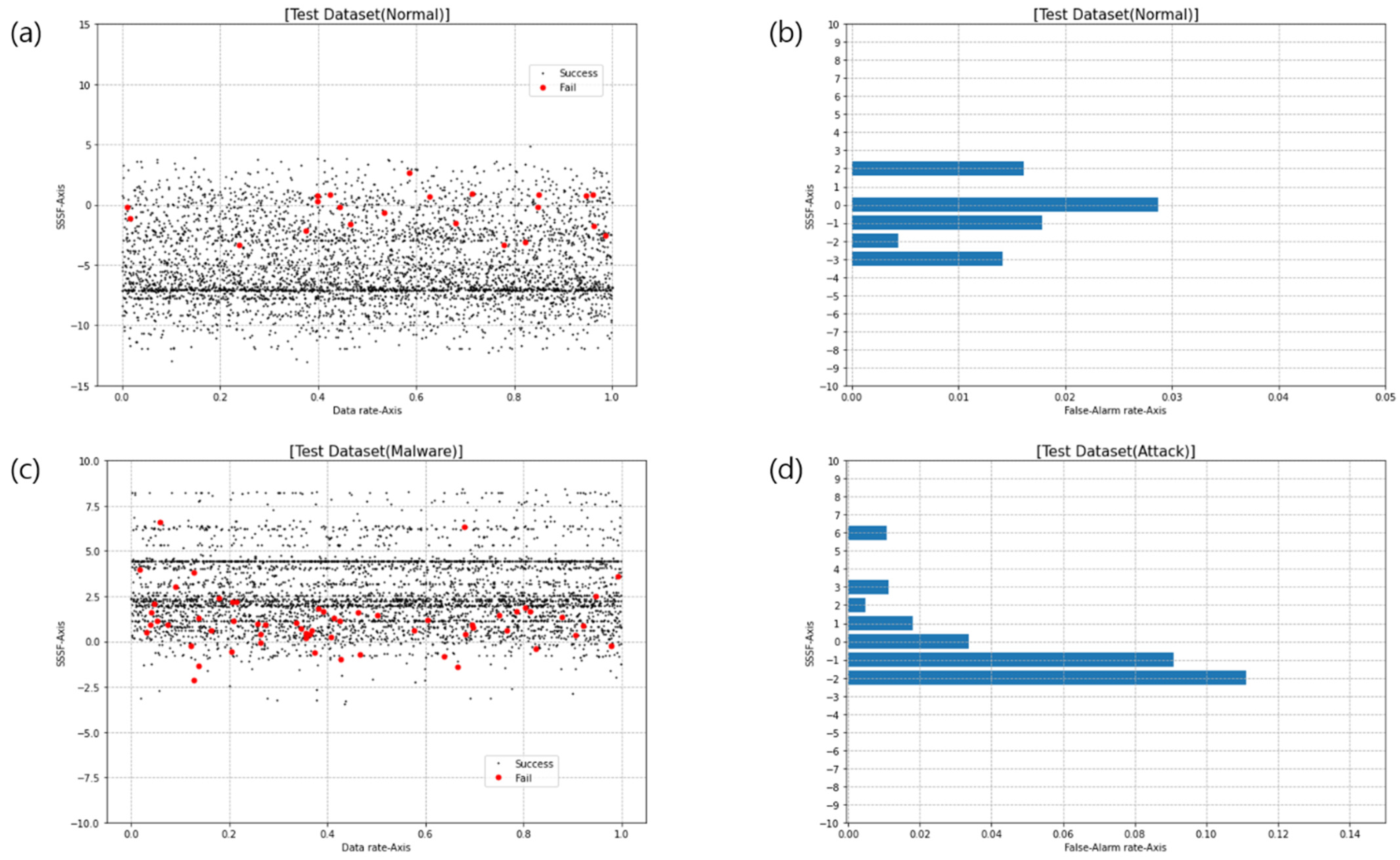
4.1. IDS Dataset Experiment

The KDD’99 dataset, which has been widely used in IDS construction, has been a popular dataset since its launch in 1999. The NSL-KDD is a dataset that has been proposed to supplement some problems in the original dataset, such as removing duplicate records from KDD’99. The labels in the NSL-KDD dataset consist of normal and four main types of attacks. This experiment combines the four attack types into one and predicts the attack types and the normal instances. The detailed composition of the NSL-KDD dataset is shown in Table 1.
Among the 41 features of the NSL-KDD dataset, the protocol type, flag, and service are configured in the form of a string. There are three types of string values for the protocol type, 11 types of string values for the flag, and 70 types of string values for the service. A one-hot encoder is used for three features to convert strings into numbers to train the AI models. Any feature to which the one-hot encoder is applied has a unique feature value. Finally, the 41 features are extended to 122. Next, for the optimization, min–max scaling is applied to all features except for six features that have binary values (“land”, “login_in”, “root_shell_su_attempted”, “is_host_login”, “is_guest_login”). This reduces the deviation between feature values and reduces the error of prediction. After applying min–max scaling, the feature is converted to a value within the range of 0 and 1.
The AI model was learned with a preprocessed training dataset. For learning, XGBoost, an ensemble algorithm that uses a combination of several decision trees, was used. The XGBoost parameters used in the experiment are shown in Table 2. Table 3 summarizes the results generated by predicting the test dataset.
We used TreeExplainer, which quickly and accurately calculated the SHAP value for the tree and tree emblems. Figure 5 is the result of generating a summary plot for each label after calculating the SHAP value of the training dataset. The summary plot shows the SHAP value for each feature value of each instance. The color is determined by the feature value, the x-axis shows the SHAP value, and the y-axis shows the distribution of instances. The left and right graphs are summary plots of the data whose labels are normal and attacks, respectively. According to the criteria described above for selecting the important features, the following 10 features were selected for each label. The important features of normal are “dst_host_srv_count”, “service_http”, “dst_host_same_srv_rate”, “logged_in”, “service_domain_u”, “Protocol_type_udp”, “srv_diff_host_rate”, “service_smtp”, “flag_REJ”, and “flag_S1.” The important features for attack are “count”, “dst_host_serror_rate”, “service_private”, “dst_host_same_src_port_rate”, “Protocol_type_icmp”, “dst_host_rerror_rate”, “hot”, “service_ecr_i”, “dst_host_diff_srv_rate”, and “dst_host_srv_diff_host_rate”. Based on the features selected in this way, SSSF is calculated with features that fit the label corresponding to the data predicted by AI. The SSSF distribution for each label is shown in Figure 6.
The first reliability analysis indicator is SSSF. The SSSF distribution of the data predicted by AI as normal in the test dataset is shown in the graph on the top left in Figure 7. In the graph, the x-axis represents the proportion of the entire dataset, and 0.1 is the data distribution corresponding to 10% of the entire dataset. The current state is a random state that is not sorted based on an indicator and just represents the order in which it was input. The SSSF of most data is distributed below 0. If the AI prediction for the data is accurate, the contribution to the attack of important features would be negative, so the SHAP value would be negative, and the SSSF would also be negative. Therefore, it can be expected that SSSF is calculated at a position less than 0 in the graph. However, on the contrary, if the SSSF is rather positive, then AI is predicted to be normal, but this means that it is considered an attack for important features. It is appropriate to judge these cases as normal based on important features that the analyst considers important but that AI judges as attacks. If an analyst re-analyzes them first, the false AI prediction can be detected in an efficient and explainable way. In Figure 6, if the analyst analyzes the data in the order of high SSSF, it is possible to detect an error with high probability. The graph on the right side of Figure 6 shows the prediction success/failure distribution. Black indicates data that are correctly predicted, and red indicates data that failed to be predicted. In fact, in the case of the data whose labels were predicted to be normal, it can be seen that prediction failure occurs more in the region where the SSSF is higher than expected. Conversely, the data predicted as an attack are expected to have a high SHAP value for important features. The corresponding SSSF will also come out high. If instances with small SSSF are analyzed first, false AI predictions can be detected with high probability.
Next, a reliability analysis is performed based on SSSF and the outlier score. The k-NN algorithm is used to calculate the outlier score by representing minute differences in the data. Based on all the features of the data, the degree of difference in other data is measured. The outlier score is the Euclidean distance between the input data and the k-th closest data in the training dataset. In this paper, k = 5 was set for the experiment.
The degree of anomaly is measured through SSSF, and the outlier score and is used as a reliability analysis indicator. The reliability score is calculated using the k-NN algorithm based on 2D data composed of SSSF and an outlier score and is not based on all features. The left graph of Figure 7 is the result of calculating the SSSF and outlier score of the normal data of the training dataset. We calculated SSSF and outlier score of the new input data. Based on these scores, the reliability score of the input data was calculated. This is to determine reliability by analyzing the general trend of the training dataset and analyzing different degrees. It is also to measure the statistical outlier of the SHAP value according to the feature value. The right graph in Figure 7 represents the distribution of the reliability scores for the data that AI predict as normal in the test dataset. The larger the statistical outlier, i.e., the farther away from the general trend of the training dataset, the higher the reliability score, and the more suspicious the judgment is. Analyzing the order of the data with large reliability scores is to analyze cases that deviate from the general trend as a priority. This enables more effective error detection.

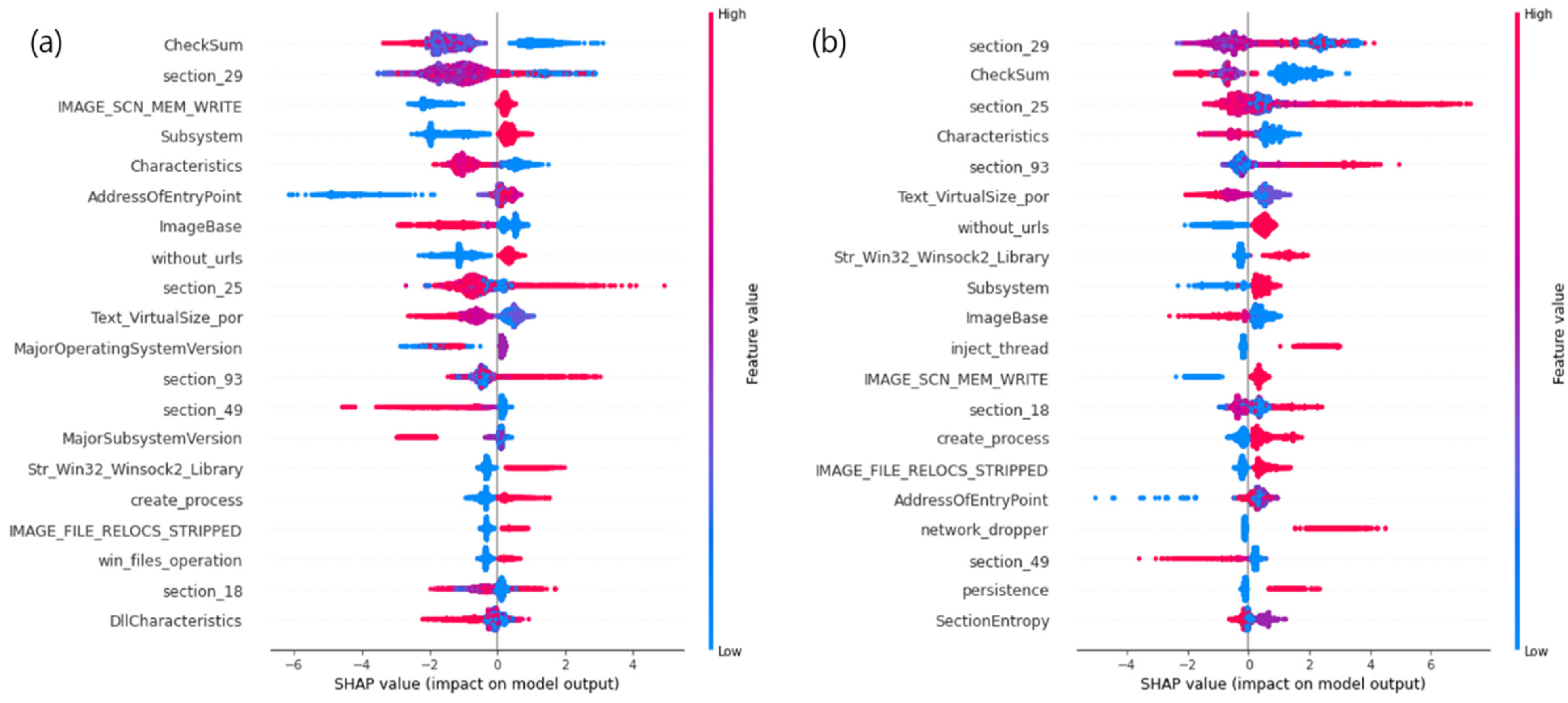
4.2. Malware Dataset Experiment

To verify the validity, an experiment was conducted using the 2019 KISA Data Challenge Dataset. The data composition of the 2019 KISA Data Challenge Dataset is the same as shown in Table 4, with the exception of a file whose features could not be extracted because the format of the PE header did not match. The malware features were extracted using PE static analysis and YARA rules [28]. YARA rules are used to classify and identify malware samples by creating descriptions of malware families based on textual or binary patterns. Through the PE static analysis, 677 features were extracted from the DLL/API, section, entropy, and PE Header, and 104 features were extracted through YARA rules matching information. A total of 781 malware features were used.
The AI learning algorithm used LightGBM, which is an ensemble algorithm similar to XGBoost. The LightGBM parameters used in the experiment are shown in Table 5. Table 6 summarizes the results generated by predicting the test dataset.
The AI that learned the malware dataset also used TreeExplainer. Figure 8 shows the results of generating a summary plot for each label after calculating the SHAP value of the training dataset. The left and right graphs are summary plots of data whose labels are normal and malware. According to the criteria for selecting the important features described above, the following 10 features were selected for each label. The important features of normal were “CheckSum”, “IMAGE_SCN_MEM_WRITE”, “Subsystem”, “Characteristics”, “AddressOfEntryPoint”, “ImageBase”, “without_urls”, “Text_VirtualSize_por”, “MajorSubsystemVersion”, and “section_49.” The important features of malware were “CheckSum”, “Characteristics”, “section_93”, “Str_Win32_Winsock2_Library”, “inject_thread”, “create_process”, “IMAGE_FILE_RELOCS_STRIPPED”, “network_dropper”, “persistence”, and “PointerToLineumbers”. Based on the features selected in this way, the SSSF was calculated with features fitting the label corresponding to the data predicted by AI.
The SSSF distribution of the data predicted by the AI as normal in the test dataset is shown in the graph on the top-left of Figure 9. It can also be seen that the SSSF of most data is distributed below 0 for the malware dataset. As with the IDS dataset, if you analyze the upper data with a high SSSF, you would be able to detect false predictions with a high probability. In fact, as shown in the graph on the top right of Figure 9, it can be seen that false predictions mainly occurred in the data with a high SSSF even though the prediction was normal.
As in the previous experiment with the IDS dataset, the k of the k-NN algorithm was set to 5 to measure the outlier score. The left graph of Figure 10 is the result of calculating the SSSF and the outlier score of the normal data on the training dataset. The right graph of Figure 10 shows the distribution of the reliability scores for the data that the AI predicted to be normal in the test dataset.

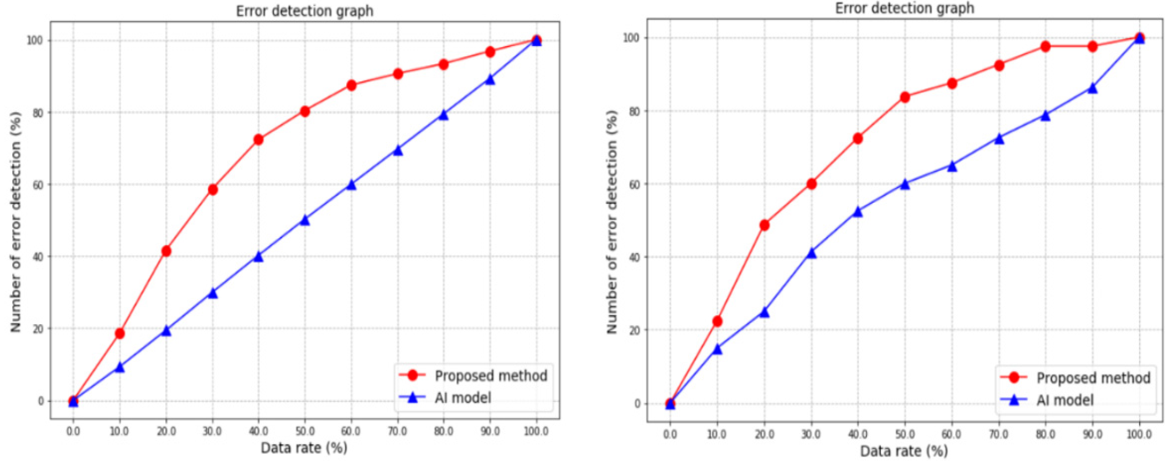
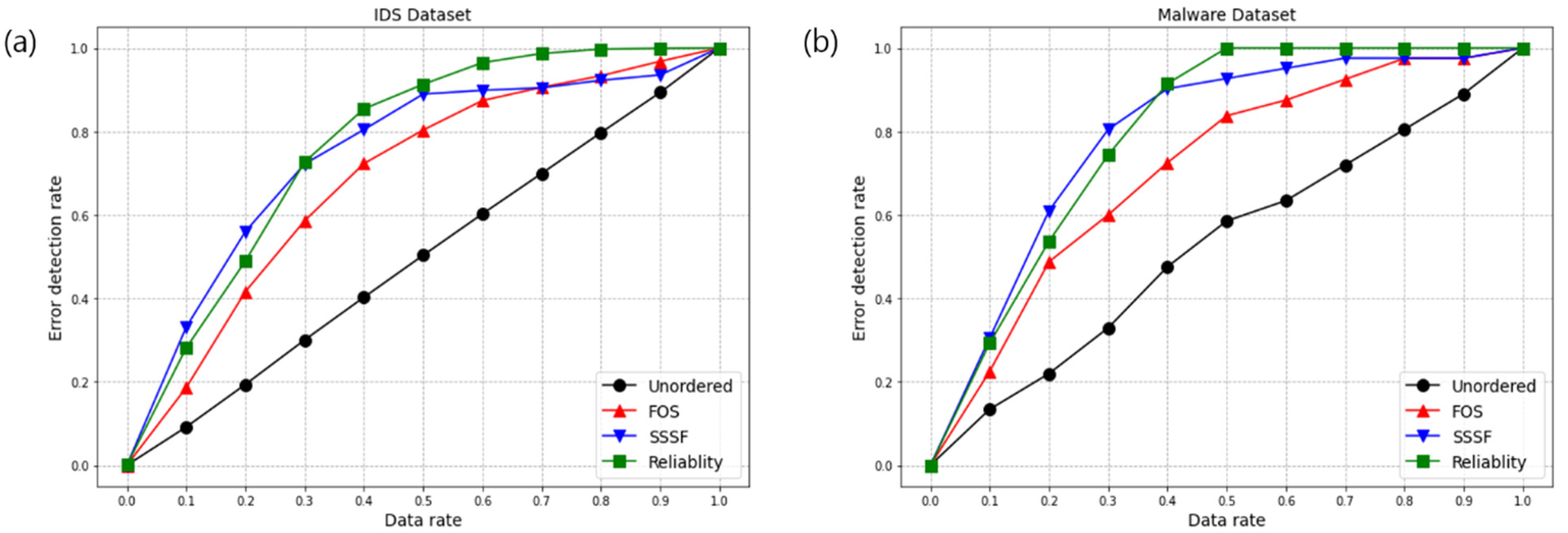
4.3. Comparative Analysis of AI Reliability Evaluation

We compared the results using the same dataset as in the previous paper. Kim et al. proposed a method for the automatic screening of valuable alerts based on XAI [25]. After the method measures the contribution of each feature of the data used for AI prediction, it selects 10 important contributing features. Then, by measuring the contribution of the features to the new input data, the method decides whether to doubt whether AI’s judgment about important features is reliable. AI judgment is analyzed using a confidence indicator called the feature outlier score (FOS). FOS is calculated based on the cumulative probability distribution of the contribution of each feature in the training dataset, and then the suspicion score for the input data is calculated and valuable alerts are selected. Experiments were conducted using the IDS dataset, NSL-KDD, the malware dataset, and the 2019 KISA Data Challenge Dataset. Figure 11 is the result of comparing the number of errors detected by the AI model with those of the proposed method. Compared to the existing AI model, the proposed method showed a 114% improvement in the IDS dataset and a 95% improvement in the malware dataset. This method has the advantage of being able to check the suspicion score for each feature, and the improved performance is insufficient for application in real environments.
Figure 12 represents a graph that compares the experimental results of the IDS dataset and the results calculated based on the FOS. Table 7 is the result of comparing the false alarms that were detected when we analyzed the upper data with high analysis priorities with data that were not ordered with priority. The performance improvement ratio according to the proposed method was calculated by comparing data that were not ordered by priority and data that were ordered by priority using each indicator. The “data rate” represents the proportion of the entire dataset. If the dataset is sorted based on the reliability score, then “data rate = 0.1” represents the top 10% of data. At the same data rate, if 10 false alarms occurred in unordered data, 16 occur in data sorted by FOS, and 20 occur in data sorted by SSSF, the improvement rate can be calculated as follows: FOS improved performance by 60% ((16 − 10)/10) over unordered data, SSSF improved performance by 100% ((20 − 10)/10) over unordered data, and SSSF improved performance by 25% ((20 − 16)/16)) over FOS. Based on the top 10% of data with high analysis priority in the IDS dataset, it was confirmed that the results calculated based on the FOS were 103%, the results calculated with the reliability score were 207%, and the results calculated with SSSF were 262%. For the malware dataset, it was confirmed that the results calculated based on FOS were 68%, the results calculated with the reliability score were 118%, and the results calculated with the SSSF were 127%.

5. Discussion

Although advanced cyber threats are increasing day by day, it is difficult to provide an accurate analysis of and response to most threats due to the lack of effective systems. AI technology is being introduced to solve these problems. However, because of opacity and reliability problems, the AI decision-making process is difficult to understand. As a result, there is a limit to introducing AI technology because it is difficult to fully trust AI predictions. Given the reliability problems of AI, analysts must analyze and process data directly after predictions by AI models. However, for a massive cyber threat, the amount of data that must be analyzed is huge, and there are far too few analysts. This makes it difficult for analysts to directly analyze the predictions of cyberthreat detection AI models and respond in a timely manner.
In this paper, we propose a method for measuring the contribution of each feature through XAI and calculating the reliability by measuring the statistical outliers of new data based on the training dataset. It was actually possible to analyze effective false alarms when using confidence indicators during analysis. The judgment of the AI model was analyzed based on the statistical outlier of the SHAP value indicating the contribution. Therefore, it is important that the XAI scores, including the SHAP value, accurately measure the contribution. It is necessary to evaluate how accurately the SHAP value actually contains the degree to which the feature contributed to AI prediction.
Currently, several XAI evaluation methods are being studied, but no definitive standard exists. It is impossible to measure the accuracy of direct contribution, but indirect measurement is possible through other XAI technologies. However, the results differ depending on the measurement method.
False alarms were able to be analyzed with higher probability compared to previous studies, but there are still disadvantages because the objective verification of the XAI score has not been performed. Further research on XAI evaluation methods is necessary to expand the effectiveness of the XAI-based framework.

6. Conclusions

The proposed method efficiently analyzes large-scale threats using XAI and can identify features that contribute significantly to the training of AI models so that even humans can easily interpret and understand the basis for AI predictions. When we carry out analyses based on the SSSF, which indicates the bias of the label, it is possible to preferentially select the data that the AI judges in disagreement to what the expert expects. This means that it is possible to examine what AI judges incorrectly from a human point of view. When we carry out analyses using the reliability score, this indicator contains sophisticated differences that may affect AI judgment. From the point of view of AI, it is possible to inspect the parts that AI can get wrong by adding indicators that can be intuitively interpreted by humans.
We conducted experiments on the IDS dataset and the malware dataset to verify the performance of the proposed method. As a result of the experiment, the analysis with SSSF and the reliability score was able to detect a false alarm two to three times more efficiently than an analysis using AI models alone. The performance improved from 30% to 80% compared to the FOS used in previous studies [24]. Excellent results were obtained not only on the IDS dataset but also on the malware dataset. Through this, it was confirmed that the proposed method is generally applicable and is not constrained by the dataset. The proposed method can efficiently detect errors in the existing AI model. The proposed method can measure the reliability of the prediction of the AI model. This enables more the efficient and accurate identification of valuable alerts, enabling more efficient workflow for human analysts. Improved identification can also enhance system performance through analysis by promoting AI model approaches in real-world environments.
The reliability indicators generated in this paper go beyond simply measuring reliability. They contain meaningful information that experts can use to analyze data. In addition to reliability, analysts can provide an environment in which efficient analysis can be performed through XAI-based analysis.

Author Contributions

Conceptualization, E.L., Y.L. and T.L.; methodology, E.L. and T.L.; software, E.L. and Y.L.; formal analysis, E.L.; investigation, E.L. and Y.L.; resources, Y.L.; writing—original draft preparation, E.L. and T.L.; writing—review and editing, E.L., Y.L. and T.L.; visualization, E.L.; supervision, T.L. All authors have read and agreed to the published version of the manuscript.

Funding

This work was supported by Institute for Information & communication Technology Planning & evaluation (IITP) grant funded by the Korean Government (MSIT) (No. 2019-0-00026, ICT infrastructure protection against intelligent malware threats).

Institutional Review Board Statement

Not applicable.

Informed Consent Statement

Not applicable.

Data Availability Statement

Not applicable.

Conflicts of Interest

The authors declare no conflict of interest.

References

  1. McAfee, Inc. McAfee Labs Threats Report: November 2020, U.S, CA. 2020. Available online: https://www.mcafee.com/enterprise/en-us/assets/reports/rp-quarterly-threats-nov-2020.pdf (accessed on 27 June 2022).
  2. Check Point Research: Cyber Attacks Increased 50% Year over Year. Available online: https://blog.checkpoint.com/2022/01/10/check-point-research-cyber-attacks-increased-50-year-over-year/ (accessed on 27 June 2022).
  3. Shapley, L.S. A value for N-person games. In Contributions to the Theory of Games; Kuhn, H.W., Tucker, A.W., Eds.; Princeton University Press: Princeton, NJ, USA, 1950; Volume I. [Google Scholar]
  4. Yang, Y.; Tresp, V.; Wunderle, M.; Fasching, P.A. Explaining Therapy Predictions with Layer-Wise Relevance Propagation in Neural Networks. In Proceedings of the 2018 IEEE International Conference on Healthcare Informatics (ICHI), New York, NY, USA, 4–7 June 2018; pp. 152–162. [Google Scholar] [CrossRef]
  5. Zafar, M.R.; Khan, N.M. DLIME: A deterministic local interpretable model-agnostic explanations approach for computer-aided diagnosis systems. arXiv 2019, arXiv:1906.10263. [Google Scholar] [CrossRef]
  6. Survey: 27 Percent of IT Professionals Receive More Than 1 Million Security Alerts Daily. Available online: https://www.imperva.com/blog/27-percent-of-it-professionals-receive-more-than-1-million-security-alerts-daily/ (accessed on 27 June 2022).
  7. Kanimozhi, V.; Jacob, T.P. Artificial Intelligence based Network Intrusion Detection with Hyper-Parameter Optimization Tuning on the Realistic Cyber Dataset CSE-CIC-IDS2018 using Cloud Computing. In Proceedings of the 2019 International Conference on Communication and Signal Processing (ICCSP), Chennai, India, 4–6 April 2019; pp. 0033–0036. [Google Scholar]
  8. Bazrafshan, Z.; Hashemi, H.; Fard, S.M.H.; Hamzeh, A. A survey on heuristic malware detection techniques. In Proceedings of the 5th Conference on Information and Knowledge Technology, Shiraz, Iran, 28–30 May 2013; pp. 113–120. [Google Scholar]
  9. Venkatraman, S.; Alazab, M.; Vinayakumar, R. A hybrid deep learning image-based analysis for effective malware detection. J. Inf. Secur. Appl. 2019, 47, 377–389. [Google Scholar] [CrossRef]
  10. Ding, Y.; Zhai, Y. Intrusion Detection System for NSL-KDD Dataset Using Convolutional Neural Networks. In Proceedings of the 2018 2nd International Conference on Computer Science and Artificial Intelligence, Shenzhen, China, 8–10 December 2018; pp. 81–85. [Google Scholar]
  11. Om, H.; Kundu, A. A hybrid system for reducing the false alarm rate of anomaly intrusion detection system. In Proceedings of the 2012 1st International Conference on Recent Advances in Information Technology(RAIT), Dhanbad, India, 15–17 March 2012; pp. 131–136. [Google Scholar]
  12. Hubballi, N.; Suryanarayanan, V. False alarm minimization techniques in signature-based intrusion detection systems: A survey. Comput. Commun. 2014, 49, 1–17. [Google Scholar] [CrossRef] [Green Version]
  13. Spathoulas, G.P.; Katsikas, S.K. Reducing false positives in intrusion detection systems. Comput. Secur. 2010, 29, 35–44. [Google Scholar] [CrossRef]
  14. Suman, R.R.; Mall, R.; Sukumaran, S.; Satpathy, M. Extracting State Models for Black-Box Software Components. J. Object Technol. 2010, 9, 79–103. [Google Scholar] [CrossRef]
  15. Amarasinghe, K.; Manic, M. Improving User Trust on Deep Neural Networks Based Intrusion Detection Systems. In Proceedings of the IECON 2018—44th Annual Conference of the IEEE Industrial Electronics Society, Washington, DC, USA, 21–23 October 2018; pp. 3262–3268. [Google Scholar]
  16. Guidotti, R.; Monreale, A.; Ruggieri, S.; Turini, F.; Giannotti, F.; Pedreschi, D. A survey of methods for explaining black box models. Assoc. Comput. Mach. 2018, 51, 1–42. [Google Scholar] [CrossRef] [Green Version]
  17. Arrieta, A.B.; Díaz-Rodríguez, N.; del Sera, J.; Bennetot, A.; Tabik, S.; Barbado, A.; Garcia, S.; Gil-Lopez, S.; Molina, D.; Benjamins, R.; et al. Explainable artificial intelligence (XAI): Concepts, taxonomies, opportunities and challenges toward responsible AI. Inf. Fusion 2020, 58, 82–115. [Google Scholar] [CrossRef] [Green Version]
  18. Arya, V.; Bellamy, R.K.E.; Chen, P.; Dhurandhar, A.; Hind, M.; Hoffman, S.C.; Houde, S.; Liao, Q.V.; Luss, R.; Mojsilovi, A. AI Explainability 360: An Extensible Toolkit for Understanding Data and Machine Learning Models. J. Mach. Learn. Res. 2020, 21, 1–6. [Google Scholar]
  19. Wexler, J.; Pushkarna, M.; Bolukbasi, T.; Wattenberg, M.; Viégas, F.; Wilson, J. The What-If Tool: Interactive Probing of Machine Learning Models. IEEE Trans. Vis. Comput. Graph. 2020, 26, 56–65. [Google Scholar] [CrossRef] [PubMed] [Green Version]
  20. Páez, A. The Pragmatic Turn in Explainable Artificial Intelligence (XAI). Minds Mach. 2019, 29, 441–459. [Google Scholar] [CrossRef] [Green Version]
  21. Gunning, D.; Aha, D. DARPA’s explainable artificial intelligence (XAI) program. AI Mag. 2019, 40, 44–58. [Google Scholar]
  22. Lundberg, S.M.; Lee, S.I. A unified approach to interpreting model predictions. In Proceedings of the Advances in Neural Information Processing Systems 30 (NIPS 2017), Long Beach, CA, USA, 4–9 December 2017; pp. 4768–4777. [Google Scholar]
  23. Movahedi, A.; Derrible, S. Interrelated Patterns of Electricity, Gas, and Water Consumption in Large-Scale Buildings. engrXiv, 2020; under review. [Google Scholar] [CrossRef] [Green Version]
  24. Wang, M.; Zheng, K.; Yang, Y.; Wang, X. An explainable machine learning framework for intrusion detection systems. IEEE Access 2020, 8, 73127–73141. [Google Scholar] [CrossRef]
  25. Kim, H.; Lee, Y.; Lee, E.; Lee, T. Cost-Effective Valuable Data Detection Based on the Reliability of Artificial Intelligence. IEEE Access 2021, 9, 108959–108974. [Google Scholar] [CrossRef]
  26. NSL-KDD. Available online: https://www.unb.ca/cic/datasets/nsl.html (accessed on 27 June 2022).
  27. 2019 KISA Data Challenge Dataset. Available online: http://datachallenge.kr/challenge19/rd-datachallenge/malware/introduction/ (accessed on 27 June 2022).
  28. YARA Rules. Available online: https://github.com/InQuest/awesome-yara (accessed on 27 June 2022).
Figure 1. Overall structure of the proposed method.
Applsci 12 06761 g001
Figure 2. Force plot to provide the explainability of a single-model prediction.
Applsci 12 06761 g002
Figure 3. Summary plot designed to display an information-dense summary of how the top features in a dataset impact the model’s output.
Applsci 12 06761 g003
Figure 4. Reliability score calculation method. (i) Test data calculated with SSSF and outlier score. (ii) Reliability score calculated based on two-dimensional data, SSSF, and outlier score.
Applsci 12 06761 g004
Figure 5. Summary plots by label in training dataset: (a) instances labeled normal in the training dataset; (b) instances labeled attack in the training dataset.
Applsci 12 06761 g005
Figure 6. Prediction success/failure distribution in SSSF of IDS dataset: (a) success/failure distribution of the data predicted as normal in the test dataset; (b) group of SSSF success/failure distribution of the data predicted as normal in the test dataset; (c) success/failure distribution of the data predicted as an attack in the test dataset; (d) group of SSSF success/failure distribution of the data predicted as an attack in the test dataset.
Applsci 12 06761 g006
Figure 7. Process of calculating the reliability score of the test dataset with the training dataset of IDS dataset: (a) SSSF/outlier score distribution calculated from the training dataset labeled normal; (b) reliability score distribution of the data predicted as normal in the test dataset.
Applsci 12 06761 g007
Figure 8. Summary plots by label in the training dataset: (a) instances labeled normal in the training dataset; (b) instances labeled attack in the training dataset.
Applsci 12 06761 g008
Figure 9. Prediction success/failure distribution in SSSF of malware dataset: (a) success/failure distribution of the data predicted as normal in the test dataset; (b) group of SSSF success/failure distribution of the data predicted as normal in the test dataset; (c) success/failure distribution of the data predicted as an attack in the test dataset; (d) group of SSSF success/failure distribution of the data predicted as an attack in the test dataset.
Applsci 12 06761 g009
Figure 10. Process of calculating the reliability score of the test dataset with the training dataset of malware dataset: (a) SSSF/outlier score distribution calculated from the training dataset labeled normal; (b) reliability score distribution of the data predicted as normal in the test dataset.
Applsci 12 06761 g010
Figure 11. The number of errors detected by the AI model and the proposed method (IDS and malware datasets) [25].
Applsci 12 06761 g011
Figure 12. Error detection results when we analyzed the data in the order of highest analysis priority: (a) results of the experiment with the IDS dataset; (b) results of the experiment with the malware dataset.
Applsci 12 06761 g012
Table 1. Composition of the NSL-KDD.
DatasetTotal No. of Instances
InstanceNormalDoSProbeU2RR2L
Train125,97367,34345,92711,65652995
Test22,544971174602421672885
Table 2. XGBoost parameters.
ParameterValueParameterValue
BoosterGbtreeSubsample1
ObjectiveBinary:logisticColsample_bytree1
Max_depth4Learning_rate0.1
Table 3. XGBoost classification results in the test dataset.
AccuracyPrecisionRecallF1 Score
0.80640.85230.80640.8055
Table 4. Composition of the 2019 KISA Data Challenge Dataset.
DatasetTotal No. of Instance
InstanceNormalMalware
Train29,13011,56817,562
Test930145184513
Table 5. LightGBM parameters.
ParameterValueParameterValue
Boosting_typegbdtLearning_rate0.08
ObjectivebinaryFeature_fraction0.9
MetricAucBagging_fraction0.8
Is_training_metricTrueBagging_freq5
Num_leaves31verbose1
Table 6. LightGBM classification results on the test dataset.
AccuracyPrecisionRecallF1 Score
0.99090.99100.99090.9909
Table 7. Error detection comparison of unordered datasets and reliability analysis results.
DatasetData RateFOSReliability Score
(Compared with FOS)
SSSF
(Compared with FOS)
IDS Dataset10%103%207% (51%)262% (78%)
20%115%153% (18%)189% (35%)
30%95%142% (24%)140% (23%)
40%80%112% (18%)100% (11%)
Malware Dataset10%68%118% (30%)127% (36%)
20%122%144% (10%)178% (25%)
30%82%126% (24%)144% (34%)
40%52%92% (26%)90% (24%)
Publisher’s Note: MDPI stays neutral with regard to jurisdictional claims in published maps and institutional affiliations.

