
Shape Optimization with a Flattening-Based Morphing Method

School of Aerospace and Mechanical Engineering, Korea Aerospace University, Goyang 10540, Korea
*
Author to whom correspondence should be addressed.
Appl. Sci. 2022, 12(13), 6565; https://doi.org/10.3390/app12136565
Submission received: 28 May 2022
/
Revised: 17 June 2022
/
Accepted: 25 June 2022
/
Published: 28 June 2022
(This article belongs to the Section Aerospace Science and Engineering)
Abstract
:In shape optimization problems, generating variously shaped designs is an important task. In this study, a new design method called the flattening-based morphing method, which can create various designs efficiently based on baseline objects, is proposed. In the flattening-based method, anchor points are defined for each baseline object to set correspondence among the baseline objects, and each baseline object is mapped to 2D parametric space in a way that places all corresponding anchor points of the baseline objects at the same location. Then, remeshing is carried out to make the baseline objects’ mesh topologically identical in the parametric space. After these remeshed baseline objects are parameterized back to the physical space, the morphed object is created by computing the positions of its vertices as a weighted sum of the baseline meshes’ vertices. When the flattening-based morphing method is applied to find the optimal shape of a blended-wing body aircraft using an artificial neural network (ANN), the aerodynamic performance enhanced optimal model with an appropriate loading capacity is successfully achieved using three baseline models. The simulation results of the baseline models and optimization results are also provided in the current study.
1. Introduction
The shapes of engineering objects are significant design factors that affect their functionality, particularly their aerodynamic aspects. For example, engineers have developed the shapes of ground vehicles for many years to reduce aerodynamic drag and increase fuel efficiency [1,2,3,4,5]. They have also attempted to reduce wind noise and increase the driving stability at high-speed operating conditions via the modification of a vehicle’s body shape [6,7,8,9]. Not only this, but designing the system’s proper configuration also becomes important for an aircraft because the shape significantly affects its performance, such as aerodynamic drag, lift, pitching moment, and stability margin [10,11,12,13].
Optimizing the shape of an object to achieve performance improvements is an iterative process that cannot be performed in a single attempt but that instead requires the initial design to be modified several times. One of the most widely used shape design methods is to parameterize the given shape (frequently called the baseline design or baseline model) by using representative variables relating to the configuration, such as length, width, or angle of the baseline model [14,15,16]. However, this shape parameterization is so simple that it cannot be used to explore a wide range of designs in the shape optimization process. Instead, representing the shape of the baseline model based on B-spline curves [17,18,19] and non-uniform rational B-splines (NURBS) [20,21,22] and searching for the optimal shape by using the control points of these entities is a better method that many researchers have been using in optimization problems [8,23,24,25,26,27,28]. Although this approach can search for a larger variety of shapes than the representative variables-based parameterization method, shape exploration is still limited and generating global and radical shape changes from the baseline design requires numerous co-constrained control points. The Free Form Deformation (FFD) [29,30] and mesh deformation using radial basis function [31,32,33] are other shape deformation methods that vary the baseline design based on the control points, but these methods not only require many design parameters in finding the optimal shapes, but unreasonable optimal shapes are sometimes given when the shape optimization is performed using these methods [34].
To overcome the disadvantages of the previous shape design methods, Oh et al. [35] propose an efficient shape design method called the design-by-morphing method. In their study, configurations of the multiple baseline models are represented in the functional space with spectral basis functions, and the coefficients of the spectral basis functions for new objects are computed to conduct morphing. When the design-by-morphing method is applied to generate the optimal head and tail shapes of a high-speed train, the authors show the usefulness of the method by creating the optimal high-speed train whose aerodynamic performance is enhanced by approximately 13.5% compared with the best-performing baseline model. Later, Kim and Oh [36] invent a multi-resolution morphing method based on the design-by-morphing method. In their method, the coefficients of the spectral basis functions of the baseline models are divided into low- and high-frequency groups, where the coefficients in the low-frequency group are likely to define the baseline models’ abstract shapes, while those in the high-frequency group are associated to the local geometric features of the models; then, they create a new design by computing new spectral coefficients in which the low-frequency coefficients are obtained by calculating the weighted sum of the low-frequency coefficients of the baseline models and the high-frequency coefficients are obtained by assigning the high-frequency coefficients of the best-performing baseline model. In the study, they apply the multi-resolution method in optimizing the shape of a hyperloop pod and discover a new design whose drag and lift are well balanced compared with the baseline models.
Despite the superiority of the design-by-morphing and multi-resolution morphing methods, applying these methods in the shape optimization problem becomes difficult when baseline models do not have star-shaped configurations. (Here, the object is called star shaped if there is an origin where the radius is single valued as a function of longitudinal and latitudinal angles [35].) This is because the previous morphing-based design methods use longitudinal and latitudinal angles as mapping variables when their shapes are parameterized using spherical harmonics. This issue may be properly handled by using a special mapping function, for example, arclength-based parameterization, when the baseline models’ configurations are transformed into the function space; however this task increases the complexity of the entire morphing process. To overcome this drawback, a new shape design method called flattening-based morphing is proposed in the current study. Unlike the previous morphing-based shape design methods, the baseline models do not need to be star-shaped objects in the proposed method. In addition, spectral basis functions do not need to represent the configurations of the baseline objects in the flattening-based morphing method because the morphing occurs directly in the physical space. In the current study, the proposed method is applied to the conceptual design of a blended-wing body (BWB) aircraft to identify its applicability in the shape optimization problem. An artificial neural network (ANN) is used to construct a surrogate model during the optimization process due to the ANN’s high prediction accuracy [37,38,39,40,41]. When the optimization is performed, the aerodynamic-performance-improved BWB with the required loading capacity is successfully achieved. Further explanation about the flattening-based method and its application is described in the next sections.
2. Flattening-Based Morphing Method
Before explaining the flattening-based morphing method, the symbols and terminologies used in the current study are described. Let us consider a baseline model whose surface is represented as triangular mesh and define this triangular mesh as M. When the mesh M is mapped to the 2D parametric space by a mapping function , the parameterized mesh of M is denoted by U. Then, the locations of the i-th vertex of M and U can be defined as and , respectively. In addition, the one-ring neighborhood of the i-th vertex, meaning the vertices that are connected to the vertex i, is defined as and the edge between the vertices i and j is defined as .
When baseline models are morphed, if their meshes are topologically the same (meaning the number of vertices and their connectivity are identical to each other), establishing one-to-one correspondences among their vertices becomes straightforward, and morphing can be easily implemented by linear interpolations among corresponding sets of baseline meshes’ vertices. However, there is no guarantee that the topologically equivalent baseline meshes will be provided. Rather, it is more reasonable to claim that the process to match the topology of the baseline meshes is required to perform morphing. In the flattening-based morphing method, this task is implemented in the parametric space because creating the topology of the baseline models is much easier in the planar space than in 3D. For a more detailed explanation, suppose two meshes (which will be referred to as Baseline models 1 and 2) are given and we want to morph them to create a new design. The first step of the proposed method is to distribute the anchor points on the baseline models. The purpose of defining anchor points is to obtain proper connections among the baseline models in the morphing process. To create a reasonably shaped new design, the geometric features of the baseline models should be matched during the morphing process. For example, when two aircraft are morphed, the leading edge of Baseline model 1 should be morphed with that of Baseline model 2. Similarly, the cockpit of Baseline model 1 should be morphed with the corresponding part of Baseline model 2. These proper connections can be secured by linking the corresponding anchor points between the baseline models. The locations of the anchor points are manually determined by a user, but it is recommended to place the anchor points where the baseline objects’ geometry features are varied, such as the ends of leading edge line and trailing edge line of the BWBs.
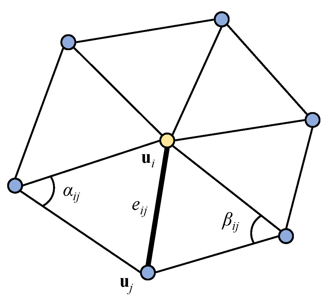
Once the anchor points have been defined, the baseline meshes are mapped to the parametric space for the remeshing. In the proposed method, a conformal mapping conceptually indicating the minimization of angle distortion between M and U is used. With a triangular mesh, the conformal mapping can be constituted by using the cotangent Laplace matrix, which can be derived by minimizing the energy over [42,43,44,45]. If the energy saved in the mesh U over is defined as E, it can be computed as
where and are the opposite angles of the edge of M and is the length of of U (see Figure 1). Minimizing E with respect to is required to find a proper mapping between M and U, which leads to the following equation:
This equation can be expressed as
in a matrix form where is the cotangent Laplace matrix of M computed by the left side of Equation (2), represents the 2D coordinate of U, and c is the zero column vector. If the boundary vertices of U are defined as and the arclength along the boundary of M and its total length are defined as l and L, respectively, solving Equation (2) with the subsequent boundary condition
allows us to parameterize the surface of M (defined in the physical space) into a unit circle.
However, when the baseline meshes are parameterized to the planar space, an anchor point should be located at the same position with its counterparts. To accomplish this, modification of the boundary condition is needed. When the anchor point is not located on the boundary, matching the position of the anchor point in the parametric space to its counterparts can be easily performed by replacing a row of the and column vector b to the Dirichlet boundary condition [46]. However, when the anchor points are located on the boundary, a special function specifying the locations of is needed. For example, let us consider the case that all anchor points are located on the boundary. Then, let us define the 2D location of the i-th anchor point in the parametric space and its 3D location in the physical space as and , respectively. Let us also define the angle measured in the parametric space between and the horizontal axis in the counter-clockwise direction as . In addition, the j-th boundary point in the parametric space and its 3D position in the physical space are defined as and , respectively. Once the angle of the first anchor point (defined as ) is set to zero, can be computed as
where is the edge length from to . Then, if the azimuthal angle of that is located between and is defined as , this can be computed as
where is the edge length between and and, is the edge length between and (see Figure 2). After computing , the boundary points in the parametric space can be obtained as
To compute , the values of need to be determined first. For this, one of the baseline models (let us use the k-th baseline model) is mapped to the parametric space with the boundary parameterization presented in Equation (4). Based on this parameterization, the azimuthal angle of the mapped k-th baseline mesh’s anchor points can be obtained from their positions. As the anchor points should be located at the same positions as their counterparts, the anchor points of other baseline models should be placed at the same locations as those of the k-th baseline model. This consequently leads to defining the values of in Equation (6), allowing us to designate the positions of the boundary points of the other baseline models in the parametric space.
As a next step, the baseline models mapped to the parametric space are remeshed to make all the mapped baseline meshes topologically identical. That is, the vertices of all the baseline meshes are located at the same positions, and their connectivity also becomes the same. This leads to securing a one-to-one correspondence among the baseline models when the remeshed baseline meshes in the parametric space are mapped back to the physical space. After the baseline models have been reconstructed from the parametric space, performing morphing among the baseline models becomes a straightforward task due to the topological consistency among the baseline models, which can be carried out as
where is the i-th vertex of the morphed model, is the weight of the j-th baseline model, and is the i-th vertex of the (remeshed) j-th baseline model. The entire process of the proposed method is described in Figure 3 with two BWB baseline models. Several examples of the morphed BWBs using the proposed method will be provided in the next section.
3. Application
In the current study, the flattening-based morphing method is applied to find an optimal shape of a BWB aircraft to identify the capability of the proposed method regarding the shape optimization problem. The knowledge necessary to conduct this optimization will be described in this section.
3.1. Baseline Models
Multiple baseline models are required to create a new design in the flattening-based morphing method. For the BWB optimization problem that is solved in the current study, the three intuition-based BWB configurations (which do not exist as real BWB models) are handled as the baseline models. The configurations of these baseline models are presented in Figure 4, along with their geometry details. In the rest of the present paper, the models presented in Figure 4a–c will be called Baseline models 1, 2, and 3, respectively.
The wingspan b of all baseline models is set to 0.93 m, but their respective lengths for Baseline models 1, 2, and 3 are 0.509, 0.577, and 0.455 m, respectively. Baseline models 1 and 2 have a large centerbody area compared to Baseline model 3, which means that they have a higher loading capacity than the latter baseline model. In fact, Baseline model 3 is a relatively thin aircraft with wide and long outer wings whose configuration is somewhat different than the other baseline models.
As presented in Equation (8), morphing among the baseline models occurs by assigning the values of the baseline models’ weights. Suppose the weights of Baseline models 1, 2, and 3 are defined as , , and , respectively. To maintain the size of a morphed model similar to that of the baseline models, the sum of all weights should be equal to 1. This condition allows us to constrain one weight to the others. In the current study, the weight of Baseline model 3 is constrained to and by
Due this relation, the morphed shape of the BWB can be controlled by two independent weights, and .
3.2. CFD Simulation
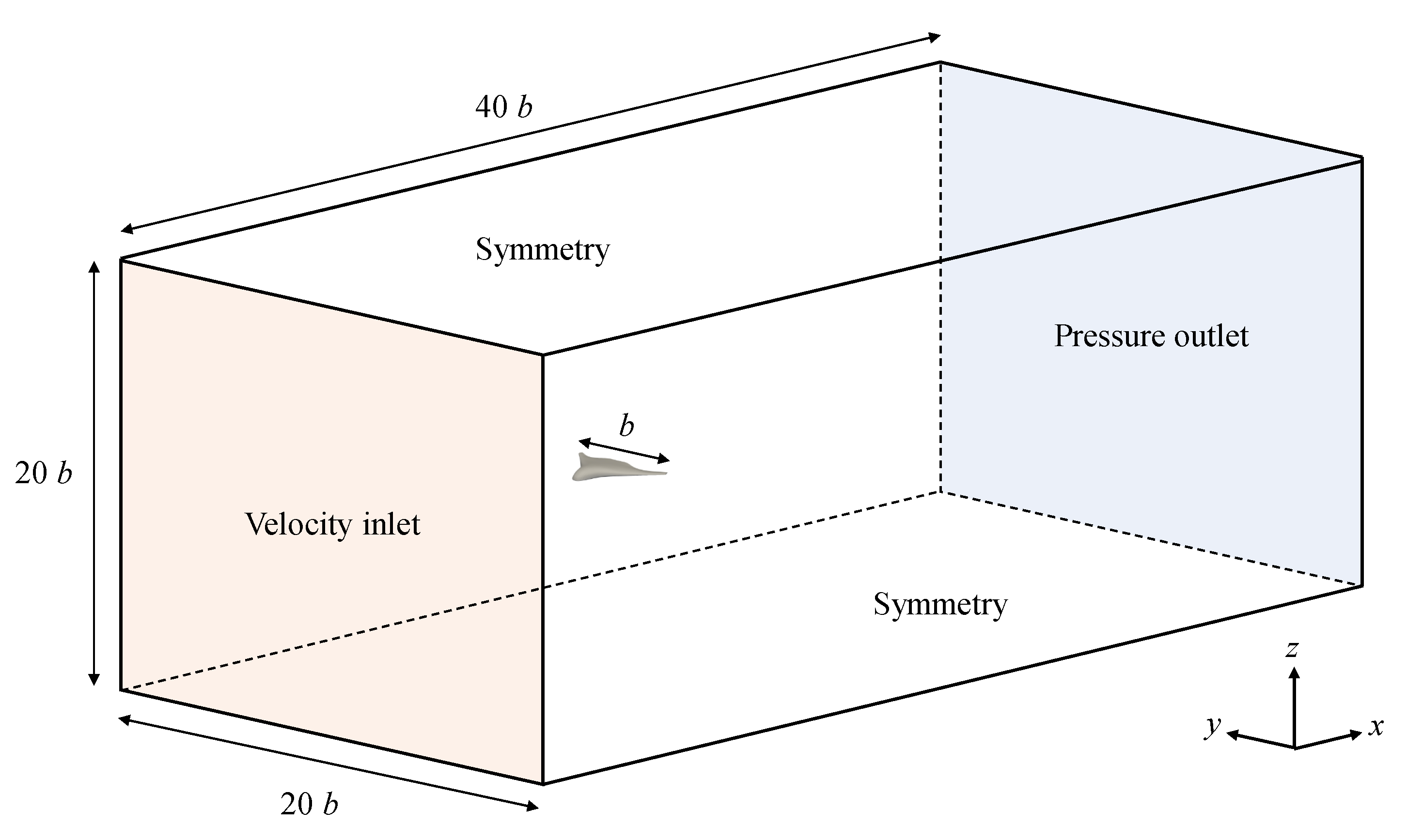
Figure 5 shows the computational domain for the BWB aircraft simulations. The flow is simulated at the freestream velocity = 27.78 m/s, which is the usual flight condition of this type of unmanned blended wing body aircraft [47]. The velocity inlet boundary and pressure outlet boundary conditions are used at the inlet and outlet of the computational domain. The no-slip boundary condition is applied on the surface of the aircraft. The symmetry boundary condition is applied at the top, bottom, front, and back sides of the computational domain. The steady Reynold-averaged Navier–Stokes (RANS) equations are solved using the Spalart–Allmaras turbulence model to compute the flow. The distribution of the grid around the aircraft is presented in Figure 6. To efficiently generate mesh elements for the simulation, the grid is refined as it approaches the aircraft. To properly capture the effect of the wall, the 20 structure inflation layers are generated near the surface of the aircraft with a 1:1 growth ratio. To solve the momentum equations, the SIMPLE algorithm is used with second-order spatial discretization schemes. When the residuals of the conservative variables are less than , the simulations are treated as converged. To simulate the flow around BWB aircraft, the open-source CFD software OpenFOAM v7 (London, United Kingdom) is used.
To analyze the reliability of the simulation, the grid sensitivity test is carried out, as presented in Table 1. The CFD simulations are conducted when the angle of attack is zero with the three types of grids (entitled to coarse, intermediate, and fine meshes). The total number of elements for the coarse-to-fine meshes is approximately 5.51, 8.75, and 13.08 million, respectively. The simulation results among these three meshes are compared with respect to the drag coefficient. The value provided in the last column of the table is the percentage of the drag coefficient difference that the corresponding mesh has compared with the fine mesh. For the coarse mesh, the relative error is computed as 2.4%. This error is reduced by up to approximately 1% at the intermediate mesh, showing the robustness of the current study’s CFD simulation. Based on the results of the grid sensitivity test, the intermediate mesh is selected for the remaining BWB’s CFD simulations.
3.3. Design Parameters and Objective Function
To optimize the configuration of the BWB, the aerodynamic performance of the aircraft should be evaluated. The lift and drag forces of the aircraft are the two most important factors affecting its performance from an aerodynamic aspect. As increasing the lift and decreasing the drag helps improve the aerodynamic performance of the aircraft, numerous researchers have considered the value of the lift-to-drag ratio to be a useful quantity for aircraft aerodynamic performance measurement [48,49,50,51]. Based on this, the current study also evaluates the aircraft’s performance based on the lift-to-drag ratio; thereby, the configuration optimization of the BWB aircraft has been implemented to maximize the lift-to-drag ratio of the morphed BWB aircraft.
The next step of the BWB optimization is to define the range of the design parameters (which are and in the current study). To properly set the ranges of the design parameters, several morphed BWBs are plotted in Figure 7 with their weights. As shown by the figure, the proposed method can generate variously shaped BWB aircraft by only considering two variables, but not every morphed BWB design is physically acceptable. For example, assigning generates a morphed BWB with a very high wing aspect ratio, which can cause structural weakness when the aircraft is put into operation (see Figure 7e). This type of aircraft tends to be generated as the sum of and increases. In addition, a thin morphed aircraft is created as decreases, and the intersection between the upper and lower surface of the morphed aircraft is detected when is smaller than (as shown by Figure 7f). To exclude these physically unacceptable morphed BWB aircraft from the design space, the ranges of and in the optimization process are restricted, as presented in Table 2. The constraint condition in the table is dealt with as two inequality constraints ( and ). These inequality constraints are handled using the augmented Lagrangian barrier algorithm when the optimization problem is solved [52].
3.4. Optimization
In the experiment design, a full factorial design was used. When this method is applied, equally spaced design points were distributed in the design space and the distance between the neighbor design points was set to 0.25 in both the and directions. This allowed us to distribute a total of 19 design points in the experiment design step (see Figure 8). At each design point, the morphed BWB aircraft was created with the flattening-based morphing method, and the CFD simulation was performed to compute its lift-to-drag ratio.
After all calculations were finished, a surrogate model computing the relation between the lift-to-drag ratio and weights was constructed using an ANN. When constructing the ANN, all 19 simulations performed in the experiment design step were used as training data. To evaluate the accuracy of the ANN with data that the ANN have never seen before, four additional simulations were performed at arbitrarily chosen design parameter’ sets (which are and , and these simulation results were used as the test data. The ANN was trained to minimize the cost function J, which is defined as
where and are the i-th lift-to-drag ratios computed from ANN and CFD, respectively, is the regularization constant, and is the vector of the neural network connectivity weights. The multi-layer perceptron approach is used to construct the neural network. The Relu function is used as the activation function, and the Adam optimizer is applied as the optimization algorithm. The regularization constant was set to , and the ANN with two hidden layers, in which each hidden layer consists of 32 neurons, was used in the optimization process. The way these ANN-related parameters were determined is described in Section 4.
After the surrogate model was constructed, an optimal set of weights that maximized the lift-to-drag ratio was searched for. As an optimization algorithm, a genetic algorithm that stochastically finds an optimal solution was used [40,53,54]. When solving the optimization problem, two geometrical constraints can be considered because these are needed to secure proper loading capacity of a new BWB aircraft. To ensure proper loading capacity, a certain amount of centerbody’s volume should be maintained for the morphed BWB aircraft. In the current study, proper volume of the centerbody was assumed to be secured by defining the lower limits of the surface area of the centerbody and cross-sectional area at the symmetry plane. With these two constraints, the optimization problem handled in the current study can be stated as
where and are the surface area of the centerbody of the morphed and reference aircraft, respectively, and are the cross-sectional areas of the morphed and reference aircraft on the symmetry plane, respectively, and is the constant that determines the relative loading capacity of the morphed aircraft compared with the reference aircraft. Baseline model 1 was used as the reference aircraft, and here the value of c was set to 0.95, implying the loading capacity of the morphed aircraft needed to at least be 95% of that of Baseline model 1.
4. Results
The distribution of the lift-to-drag ratio over the design space is illustrated in Figure 9. The lift-to-drag ratio of Baseline model 1 (at ) is measured as 3.885, while that of Baseline model 2 (at ) is approximately 5.926. Although Baseline model 3, whose the weights are , shows the highest lift-to-drag ratio among the baseline models, its loading capacity is so low that it fails to satisfy the constraints presented in Equation (11), indicating that this type of aircraft design cannot be an optimal shape. In the design space, the high lift-to-drag ratio region is found around the left top corners. From this observation, an optimal solution can be found close to this region if the constraints related to the aircraft loading capacity are satisfied at the region. In addition, when the change in the BWB aircraft’s performance is analyzed as a function of the design parameters, a moderate inverse proportion between the lift-to-drag ratio and is observed, as shown by Figure 10. When this distribution is modeled using a linear regression analysis, the regression model () is obtained, here with an R-squared value . However, unlike , no apparent association of with the lift-to-drag ratio is found.
When an ANN-based surrogate model is constructed, the ANN-related parameters, such as number of neurons, number of hidden layers, and value of the regularization constant, are important factors that affect the predication accuracy of the surrogate model. To find the proper values of these parameters, numerical investigations are performed by varying these parameters’ values; here, the change in the ANN’s prediction accuracy is analyzed. For the ANN-related parameters, three parameters (number of neurons, number of hidden layers, and value of regularization constant) are chosen, and the effects of these parameters on the prediction accuracy are investigated. If the number of neurons, number of hidden layers, and regularization constant are defined as N, M, and , respectively, numerical studies are conducted at 5 Ns (8, 16, 32, 64, and 128), 4 Ms (1, 2, 3, and 4), and 4 s (0.1, 0.01, 0.001, and 0.0001), totaling 80 cases. When M is greater than 1 (meaning that multiple hidden layers are used in constructing the ANN), the number of neurons at each hidden layer is defined as being equal so as to reduce the complexity of the analysis (see Figure 11). Based on the numerical investigations, the proper values of the ANN-related parameters are determined based on the following steps: First, the effect of is studied with the 80 numerical cases, and the best value of is determined. Then, by fixing the value of , the influences of M are identified, and its best value is decided. After this, the best value of N is searched for while fixing the values of and M to their best values. The prediction error of the constructed ANN is evaluated by using the norm.
The values of obtained only with test data sets are used for predicting ANN accuracy, because obtained with the training data sets is not a good measurement for the prediction accuracy due to the possibility of the overfitting.
Figure 12 shows the influence of ANN-related parameters on the prediction accuracy. To identify the influence of the regularization constant on ANN accuracy, the prediction error (measured by the averaged value of ) of the 80 test cases is plotted with respect to in Figure 12a. No clear difference of the error is observed at , 0.01, or 0.001, but the best regularization constant is set at 0.001 in the current study because a slightly smaller error is measured at compared with the other cases. Based on this result, the variation of the prediction accuracy is investigated as a function of M while fixing to 0.001. As shown in Figure 12b, the influence of M on the prediction accuracy is certainly more distinguishable than that of , and the best value of M is set to 3 based on the results. Finally, the graph plotted in Figure 12c presents the change of the prediction accuracy with respect to N when and . As the smallest error is obtained at , the 32 neurons are distributed at each hidden layer when the surrogate model is constructed. With these ANN-related parameters, the training data error is , while the test data error is , demonstrating the high prediction accuracy of the current study’s constructed surrogate model (see Figure 13).
To find the optimal shape of the BWB aircraft, the iterative optimization step is used, as shown in Figure 14. Once the ANN-based surrogate model is constructed with the simulation results of the design of experiment, an optimal set of the weights maximizing the lift-to-drag ratio are searched for over the design space using the genetic algorithm. Then, with the searched optimal set of weights, a morphed BWB aircraft is created using the flattening-based morphing method, and the CFD simulation is carried out to compute the lift-to-drag ratio. After doing this, the optimal set of weights and its lift-to-drag ratio is added to the training data sets; then, the surrogate model is updated. An optimal solution is computed again, and the process is repeated until the loop reaches the maximum iteration number. In the current study, the maximum iteration number for this optimization loop is set to 5.
Table 3 shows the changes of the optimal sets of weights during the iterative optimization process. For all the optimization iterations, is almost fixed to , while slightly varies from 0.775 to 0.805. The fourth and fifth columns from the left show the ANN-computed and CFD-computed lift-to-drag ratios, respectively, and the rightmost column presents their percentage difference compared with the CFD-computed lift-to-drag ratio. Although the monotonical decrease in the discrepancy between the ANN-computed and CFD-computed lift-to-drag ratio is not observed, the discrepancy tends to reduce as the optimization iteration number increases, indicating that the prediction accuracy of the constructed ANN is improved as the optimization loop repeats. Due to the improvement of the ANN’s prediction accuracy, the lift-to-drag ratio of the optimal models become better in the optimization step. When the optimization loop has been completed, the best performing optimal model is found at and , for which the lift-to-drag ratio is about 6.703. When the computational times for conducting CFD simulations and constructing the surrogate model are compared (approximately 4 h vs. less than a minute when the computational times are measured using a 32 GB RAM and 16-core computer), applying ANN is a highly efficient way of solving the BWB shape optimization problem.
Figure 15 demonstrates the pressure on the surfaces of the baseline and optimal models. For each figure, the left half of the plot presents the pressure on the upper surface, while the right half shows this on the lower surface. Among the baseline models, Baseline model 3 shows the widest high-pressure region on the rear of the lower surface compared with the others, which is the one factor that increases the lift at Baseline model 3. When the pressure distribution of the optimal model is analyzed, the aerodynamic advantage of Baseline model 3 is also investigated for the optimal model. Although the configuration of the optimal model is the most like that of Baseline model 2, the optimal model has a wider high pressure area, especially in the lower surface, compared to Baseline model 2’s case. Rather, the optimal model’s pressure distribution is similar to that of Baseline model 3, which shows the highest lift-to-drag ratio among the baseline models. This phenomenon indicates that the flattening-based morphing method generates the optimal shape by finding the weights that can retain the beneficial aerodynamic characteristic of the baseline models. To identify this feature more specifically, when the pressure coefficients of Baseline model 2 and the optimal model are compared at the symmetry plane, most of the lift increment at the optimal model is caused by the high pressure on the rear of the lower surface, which is the same phenomenon detected in Baseline model 3 (see Figure 16).
5. Conclusions
A new shape design method called flattening-based morphing is proposed and applied in finding the optimal shape of a BWB aircraft. In the proposed method, the anchor points that guide the geometrical correspondences among the baseline models are defined, and each baseline model is mapped to the parametric space by constructing the cotangent Laplace matrix. When the baseline models are transformed, the anchor points are constrained to be located at the specified positions to place all corresponding anchor points of the baseline models at the same positions in the parametric space. Then, the parameterized baseline meshes are remeshed to make them topologically identical. Mapping the remeshed baseline meshes back to the physical space allows us to find the one-to-one correspondence of the vertices among the baseline models. Due to this correspondence, the creation of a morphed object can be straightforwardly conducted as the interpolation of the baseline meshes’ vertices. In the current study, the flattening-based morphing method has been applied to the shape optimization of a BWB aircraft. An ANN is used to search for the association between the input and output parameters of the optimization problem. Based on the prediction accuracy test, an ANN with two hidden layers, each consisting of 32 neurons, is constructed. To prevent overfitting of the training data sets, a regularization constant (whose value is 0.001) is used to define the cost function of the ANN. During the optimization loop, a reduction in the discrepancy between the ANN-computed and CFD-computed lift-to-drag ratios is detected, showing improvement in the ANN’s prediction accuracy as the optimization loop is repeated. As a result of the optimization, an enhanced aerodynamic performance BWB model with the proper loading capacity can be successfully obtained. When the pressure distribution on the baseline and optimal models are compared, the beneficial feature of Baseline model 3 (which shows the highest lift-to-drag ratio among the baseline models) is also found at the optimal model, even though the configuration of the optimal model is the most similar to that of Baseline model 2. This indicates that the flattening-based morphing method creates an optimal shape that can retain the beneficial feature of its baseline models. As the flattening-based morphing method has an advantage in morphing complicated-shaped baseline models over previous morphing-based shape design methods, the proposed method can extend the application areas of the morphing-based shape optimization technique.
Author Contributions
Conceptualization, S.O.; Data curation, H.K.; Formal analysis, H.K. and S.O.; Funding acquisition, S.O.; Investigation, H.K.; Methodology, S.O.; Project administration, S.O.; Resources, S.O.; Software, H.K.; Supervision, S.O.; Validation, H.K.; Visualization, H.K.; Writing—original draft, H.K. and S.O.; Writing—review & editing, S.O. All authors have read and agreed to the published version of the manuscript.
Funding
This work was supported by 2020 Korea Aerospace University faculty research grant.
Conflicts of Interest
The authors declare no conflict of interest.
References
- Sun, Z.; Yao, S.; Yang, G. Research on aerodynamic optimization of high-speed train’s slipstream. Eng. Appl. Comput. Fluid Mech. 2020, 14, 1106–1127. [Google Scholar] [CrossRef]
- Sudin, M.N.; Abdullah, M.A.; Shamsuddin, S.A.; Ramli, F.R.; Tahir, M.M. Review of research on vehicles aerodynamic drag reduction methods. Int. J. Mech. Mechatron. Eng. 2014, 14, 37–47. [Google Scholar]
- Lyu, Z.; Martins, J.R. Aerodynamic shape optimization of an adaptive morphing trailing-edge wing. J. Aircr. 2015, 52, 1951–1970. [Google Scholar] [CrossRef] [Green Version]
- Guerrero, A.; Castilla, R.; Eid, G. A numerical aerodynamic analysis on the effect of rear underbody diffusers on road cars. Appl. Sci. 2022, 12, 3763. [Google Scholar] [CrossRef]
- Sun, Z.; Yao, S.; Wei, L.; Yao, Y.; Yang, G. Numerical Investigation on the Influence of the Streamlined Structures of the High-Speed Train’s Nose on Aerodynamic Performances. Appl. Sci. 2021, 11, 784. [Google Scholar] [CrossRef]
- Ju, S.; Sun, Z.; Guo, D.; Yang, G.; Wang, Y.; Yan, C. Aerodynamic-Aeroacoustic Optimization of a Baseline Wing and Flap Configuration. Appl. Sci. 2022, 12, 1063. [Google Scholar] [CrossRef]
- Maizi, M.; Mohamed, M.; Dizene, R.; Mihoubi, M. Noise reduction of a horizontal wind turbine using different blade shapes. Renew. Energy 2018, 117, 242–256. [Google Scholar] [CrossRef]
- Sanaye, S.; Hassanzadeh, A. Multi-objective optimization of airfoil shape for efficiency improvement and noise reduction in small wind turbines. J. Renew. Sustain. Energy 2014, 6, 053105. [Google Scholar] [CrossRef] [Green Version]
- Sun, C.; Song, B.; Wang, P. Parametric geometric model and shape optimization of an underwater glider with blended-wing-body. Int. J. Nav. Archit. Ocean Eng. 2015, 7, 995–1006. [Google Scholar] [CrossRef] [Green Version]
- Jha, A.K.; Kudva, J.N. Morphing aircraft concepts, classifications, and challenges. In Proceedings of the Smart Structures and Materials 2004: Industrial and Commercial Applications of Smart Structures Technologies, San Diego, CA, USA, 14–18 March 2004; International Society for Optics and Photonics: Bellingham, WA, USA, 2004; Volume 5388, pp. 213–224. [Google Scholar]
- Wang, Y.; Shen, S.; Li, G.; Huang, D.; Zheng, Z. Investigation on aerodynamic performance of vertical axis wind turbine with different series airfoil shapes. Renew. Energy 2018, 126, 801–818. [Google Scholar] [CrossRef]
- Peifeng, L.; Zhang, B.; Yingchun, C.; Changsheng, Y.; Yu, L. Aerodynamic design methodology for blended wing body transport. Chin. J. Aeronaut. 2012, 25, 508–516. [Google Scholar]
- Panagiotou, P.; Yakinthos, K. Parametric aerodynamic study of Blended-Wing-Body platforms at low subsonic speeds for UAV applications. In Proceedings of the 35th AIAA Applied Aerodynamics Conference, Denver, CO, USA, 5–9 June 2017; p. 3737. [Google Scholar]
- Brujic, D.; Ristic, M.; Mattone, M.; Maggiore, P.; De Poli, G.P. CAD based shape optimization for gas turbine component design. Struct. Multidiscip. Optim. 2010, 41, 647–659. [Google Scholar] [CrossRef]
- Sun, J.; Frazer, J.H.; Mingxi, T. Shape optimisation using evolutionary techniques in product design. Comput. Ind. Eng. 2007, 53, 200–205. [Google Scholar] [CrossRef]
- Luo, X.; Yang, B.; Sheng, L.; Chen, J.; Li, H.; Xie, L.; Chen, G.; Yu, M.; Guo, W.; Tian, W. CAD based design sensitivity analysis and shape optimization of scaffolds for bio-root regeneration in swine. Biomaterials 2015, 57, 59–72. [Google Scholar] [CrossRef]
- Gordon, W.J.; Riesenfeld, R.F. B-spline curves and surfaces. In Computer Aided Geometric Design; Elsevier: Amsterdam, The Netherlands, 1974; pp. 95–126. [Google Scholar]
- Boehm, W. Inserting new knots into B-spline curves. Comput.-Aided Des. 1980, 12, 199–201. [Google Scholar] [CrossRef]
- Farin, G.; Rein, G.; Sapidis, N.; Worsey, A.J. Fairing cubic B-spline curves. Comput. Aided Geom. Des. 1987, 4, 91–103. [Google Scholar] [CrossRef]
- Piegl, L. On NURBS: A survey. IEEE Comput. Graph. Appl. 1991, 11, 55–71. [Google Scholar] [CrossRef]
- Xie, W.C.; Zou, X.F.; Yang, J.D.; Yang, J.B. Iteration and optimization scheme for the reconstruction of 3D surfaces based on non-uniform rational B-splines. Comput.-Aided Des. 2012, 44, 1127–1140. [Google Scholar] [CrossRef]
- Liang, Y.; Cheng, X.; Li, Z.; Xiang, J. Multi-objective robust airfoil optimization based on non-uniform rational B-spline (NURBS) representation. Sci. China Technol. Sci. 2010, 53, 2708–2717. [Google Scholar] [CrossRef]
- Tang, P.S.; Chang, K.H. Integration of topology and shape optimization for design of structural components. Struct. Multidiscip. Optim. 2001, 22, 65–82. [Google Scholar] [CrossRef]
- Han, X.; Zingg, D.W. An adaptive geometry parametrization for aerodynamic shape optimization. Optim. Eng. 2014, 15, 69–91. [Google Scholar] [CrossRef]
- Qian, X. Full analytical sensitivities in NURBS based isogeometric shape optimization. Comput. Methods Appl. Mech. Eng. 2010, 199, 2059–2071. [Google Scholar] [CrossRef]
- Painchaud-Ouellet, S.; Tribes, C.; Trepanier, J.Y.; Pelletier, D. Airfoil shape optimization using NURBS representation under thickness constraint. In Proceedings of the 42nd AIAA Aerospace Sciences Meeting and Exhibit, Reno, NV, USA, 5–9 January 2004; p. 1095. [Google Scholar]
- Yu, G.; Müller, J.D.; Jones, D.; Christakopoulos, F. CAD-based shape optimisation using adjoint sensitivities. Comput. Fluids 2011, 46, 512–516. [Google Scholar] [CrossRef]
- Samareh, J. Aerodynamic shape optimization based on free-form deformation. In Proceedings of the 10th AIAA/ISSMO multidisciplinary analysis and optimization conference, Albany, NY, USA, 30 August–1 September 2004; p. 4630. [Google Scholar]
- Sederberg, T.W.; Parry, S.R. Free-form deformation of solid geometric models. In Proceedings of the 13th Annual Conference on Computer Graphics and Interactive Techniques, Dallas, TX, USA, 18–22 August 1986; pp. 151–160. [Google Scholar]
- Lyu, Z.; Martins, J.R. Aerodynamic design optimization studies of a blended-wing-body aircraft. J. Aircr. 2014, 51, 1604–1617. [Google Scholar] [CrossRef] [Green Version]
- Allen, C.B.; Rendall, T. CFD-based optimization of hovering rotors using radial basis functions for shape parameterization and mesh deformation. Optim. Eng. 2013, 14, 97–118. [Google Scholar] [CrossRef]
- De Boer, A.; Van der Schoot, M.S.; Bijl, H. Mesh deformation based on radial basis function interpolation. Comput. Struct. 2007, 85, 784–795. [Google Scholar] [CrossRef]
- Jakobsson, S.; Amoignon, O. Mesh deformation using radial basis functions for gradient-based aerodynamic shape optimization. Comput. Fluids 2007, 36, 1119–1136. [Google Scholar] [CrossRef]
- Sieger, D.; Menzel, S.; Botsch, M. On shape deformation techniques for simulation-based design optimization. In New Challenges in Grid Generation and Adaptivity for Scientific Computing; Springer: Berlin/Heidelberg, Germany, 2015; pp. 281–303. [Google Scholar]
- Oh, S.; Jiang, C.H.; Jiang, C.; Marcus, P.S. Finding the optimal shape of the leading-and-trailing car of a high-speed train using design-by-morphing. Comput. Mech. 2018, 62, 23–45. [Google Scholar] [CrossRef]
- Kim, H.; Oh, S. Shape optimization of a hyperloop pod’s head and tail using a multi-resolution morphing method. Int. J. Mech. Sci. 2022, 223, 107227. [Google Scholar] [CrossRef]
- Karimmaslak, H.; Najafi, B.; Band, S.S.; Ardabili, S.; Haghighat-Shoar, F.; Mosavi, A. Optimization of performance and emission of compression ignition engine fueled with propylene glycol and biodiesel–diesel blends using artificial intelligence method of ANN-GA-RSM. Eng. Appl. Comput. Fluid Mech. 2021, 15, 413–425. [Google Scholar] [CrossRef]
- Oh, S. Comparison of a response surface method and artificial neural network in predicting the aerodynamic performance of a wind turbine airfoil and its optimization. Appl. Sci. 2020, 10, 6277. [Google Scholar] [CrossRef]
- Seo, Y.M.; Pandey, S.; Lee, H.U.; Choi, C.; Park, Y.G.; Ha, M.Y. Prediction of heat transfer distribution induced by the variation in vertical location of circular cylinder on Rayleigh-Bénard convection using artificial neural network. Int. J. Mech. Sci. 2021, 209, 106701. [Google Scholar] [CrossRef]
- Yoo, S.; Oh, S. Flow analysis and optimization of a vertical axis wind turbine blade with a dimple. Eng. Appl. Comput. Fluid Mech. 2021, 15, 1666–1681. [Google Scholar] [CrossRef]
- Varrecchia, T.; De Marchis, C.; Draicchio, F.; Schmid, M.; Conforto, S.; Ranavolo, A. Lifting activity assessment using kinematic features and neural networks. Appl. Sci. 2020, 10, 1989. [Google Scholar] [CrossRef] [Green Version]
- Pinkall, U.; Polthier, K. Computing discrete minimal surfaces and their conjugates. Exp. Math. 1993, 2, 15–36. [Google Scholar] [CrossRef]
- Desbrun, M.; Meyer, M.; Alliez, P. Intrinsic parameterizations of surface meshes. In Proceedings of the Computer Graphics Forum; Wiley Online Library: Hoboken, NJ, USA, 2002; Volume 21, pp. 209–218. [Google Scholar]
- Oh, S. A new triangular mesh repairing method using a mesh distortion energy minimization-based mesh flattening method. Adv. Eng. Softw. 2019, 131, 48–59. [Google Scholar] [CrossRef]
- Sorkine, O. Laplacian mesh processing. Eurographics (State Art Rep.) 2005, 4. [Google Scholar] [CrossRef]
- Karim, R.; Ma, Y.; Jang, M.; Housden, R.J.; Williams, S.E.; Chen, Z.; Ataollahi, A.; Althoefer, K.; Rinaldi, C.A.; Razavi, R.; et al. Surface flattening of the human left atrium and proof-of-concept clinical applications. Comput. Med. Imaging Graph. 2014, 38, 251–266. [Google Scholar] [CrossRef] [PubMed] [Green Version]
- Dehpanah, P.; Nejat, A. The aerodynamic design evaluation of a blended-wing-body configuration. Aerosp. Sci. Technol. 2015, 43, 96–110. [Google Scholar] [CrossRef]
- Siouris, S.; Qin, N. Study of the effects of wing sweep on the aerodynamic performance of a blended wing body aircraft. Proc. Inst. Mech. Eng. Part G J. Aerosp. Eng. 2007, 221, 47–55. [Google Scholar] [CrossRef]
- Giguere, P.; Dumas, G.; Lemay, J. Gurney flap scaling for optimum lift-to-drag ratio. AIAA J. 1997, 35, 1888–1890. [Google Scholar] [CrossRef]
- Haryanto, I.; Utomo, T.S.; Sinaga, N.; Rosalia, C.A.; Putra, A.P. Optimization of maximum lift to drag ratio on airfoil design based on artificial neural network utilizing genetic algorithm. In Applied Mechanics and Materials; Trans Tech Publ: Zurich, Switzerland, 2014; Volume 493, pp. 123–128. [Google Scholar]
- Fatehi, M.; Nili-Ahmadabadi, M.; Nematollahi, O.; Minaiean, A.; Kim, K.C. Aerodynamic performance improvement of wind turbine blade by cavity shape optimization. Renew. Energy 2019, 132, 773–785. [Google Scholar] [CrossRef]
- Conn, A.; Gould, N.; Toint, P. A globally convergent Lagrangian barrier algorithm for optimization with general inequality constraints and simple bounds. Math. Comput. 1997, 66, 261–288. [Google Scholar] [CrossRef]
- Wang, S.; Jian, G.; Xiao, J.; Wen, J.; Zhang, Z. Optimization investigation on configuration parameters of spiral-wound heat exchanger using Genetic Aggregation response surface and Multi-Objective Genetic Algorithm. Appl. Therm. Eng. 2017, 119, 603–609. [Google Scholar] [CrossRef]
- Mirjalili, S. Genetic algorithm. In Evolutionary Algorithms and Neural Networks; Springer: Berlin/Heidelberg, Germany, 2019; pp. 43–55. [Google Scholar]
Figure 1.
The vertex i and its one-ring neighborhood vertices are represented as yellow and blue points. The edge between the vertices i and j is denoted by , and two opposite angles of are defined as and .
Figure 1.
The vertex i and its one-ring neighborhood vertices are represented as yellow and blue points. The edge between the vertices i and j is denoted by , and two opposite angles of are defined as and .

Figure 2.
Notations related to the boundary points. The j-th boundary point of U and i-th anchor point located on the boundary are defined as and , respectively. Their azimuthal angles are defined as and , respectively, in the current study.
Figure 2.
Notations related to the boundary points. The j-th boundary point of U and i-th anchor point located on the boundary are defined as and , respectively. Their azimuthal angles are defined as and , respectively, in the current study.

Figure 3.
The diagram of the flattening-based morphing method. After the anchor points have been defined on the baseline models, the baseline meshes are mapped to the parametric space by matching the location of the anchor points with their counterparts. Then, the mapped baseline meshes are remeshed to make them topologically the same. The remeshed baseline models are parameterized back to the physical space, and a new morphed model is created by interpolating the configuration of the remeshed baseline models. Here, for BWB morphing, the upper and lower sides of the BWB are separately mapped to the parametric space.

Figure 4.
The configurations of the three baseline BWB aircraft. (a) Baseline model 1, (b) Baseline model 2, and (c) Baseline model 3.
Figure 4.
The configurations of the three baseline BWB aircraft. (a) Baseline model 1, (b) Baseline model 2, and (c) Baseline model 3.

Figure 5.
Computational domain for the BWB aircraft CFD simulation with boundary conditions.

Figure 6.
The computational mesh around the BWB aircraft. The red boxed area in (a) is magnified in (b).
Figure 6.
The computational mesh around the BWB aircraft. The red boxed area in (a) is magnified in (b).

Figure 7.
Several BWB aircraft created with the flattening-based morphing method. The weights of each morphed BWB aircraft are presented in the caption. The weights of the aircraft plotted in (a–d) exist in the current study’s design space, but the ones plotted in (e,f) are located outside of the design space.

Figure 8.
The illustration of the design space with 19 initial design points. The bold black lines show the design space of the optimization problem, while the black dotted points are the 19 design points in the design of experiment.
Figure 8.
The illustration of the design space with 19 initial design points. The bold black lines show the design space of the optimization problem, while the black dotted points are the 19 design points in the design of experiment.

Figure 9.
Distribution of the lift-to-drag ratio in the design space.

Figure 10.
Correlation between and . The black dots show the lift-to-drag ratio of the 19 design points at the design of experiment and four test data sets. The red line shows the linear regression model computed with data from the 23 simulations. The R-squared value of this regression model is , representing a moderate correlation between and .

Figure 11.
Structure of the constructed ANN. The number of hidden layers and neurons at each hidden layer are defined as M and N, respectively. Using the ANN, the value of the lift-to-drag ratio is predicted as a function of and .
Figure 11.
Structure of the constructed ANN. The number of hidden layers and neurons at each hidden layer are defined as M and N, respectively. Using the ANN, the value of the lift-to-drag ratio is predicted as a function of and .

Figure 12.
The influence of the ANN-related parameters on its prediction accuracy. (a) Regularization constant, (b) number of hidden layers, and (c) number of neurons.
Figure 12.
The influence of the ANN-related parameters on its prediction accuracy. (a) Regularization constant, (b) number of hidden layers, and (c) number of neurons.

Figure 13.
The accuracy of the ANN in predicting the CFD-computed lift-to-drag ratio. The black dots are the 19 data sets used to train the ANN, while the red dots are four test data sets used to measure the ANN’s accuracy. The R-squared values of the training data sets and test data sets with a 45 line are 0.9992 and 0.9643, respectively.

Figure 14.
Flow chart of the iterative optimization process.

Figure 15.
The distributions of the pressure on the surfaces of the baseline and optimal models. For each figure, the left and right contours show the pressure on the upper and lower surfaces of the BWB aircraft, respectively. (a) Baseline model 1, (b) Baseline model 2, (c) Baseline model 3, and (d) the optimal model.

Figure 16.
The pressure coefficients of Baseline model 2 and optimal model at the symmetry plane. The solid and dashed lines present the pressure coefficient on the upper and lower surfaces, respectively.
Figure 16.
The pressure coefficients of Baseline model 2 and optimal model at the symmetry plane. The solid and dashed lines present the pressure coefficient on the upper and lower surfaces, respectively.


Table 1.
Results of the grid sensitivity test. The “relative error” in the last column presents the percentage of the drag coefficient difference that the corresponding mesh has compared with the fine mesh.
Table 1.
Results of the grid sensitivity test. The “relative error” in the last column presents the percentage of the drag coefficient difference that the corresponding mesh has compared with the fine mesh.
| Meshes | Number of Cells () | Number of Layers | Averaged | First Layer Thickness ( m) | Drag Coefficients | Relative Error (%) |
|---|---|---|---|---|---|---|
| Coarse | 5.51 | 20 | 2.36 | 3.58 | 0.01492 | 2.40 |
| Intermediate | 8.75 | 20 | 2.09 | 3.17 | 0.01473 | 1.10 |
| Fine | 13.08 | 20 | 1.82 | 2.76 | 0.01457 | - |
Table 2.
Bounds and constraint of the design parameters.
| Parameters | Lower Bounds | Upper Bounds |
|---|---|---|
| 1 | ||
| 1 | ||
| Constraint | 0 1 | |
Table 3.
Evolution of the optimization results during the optimization loop. The “error” in the last row shows the percentage difference between the ANN-computed and CFD-computed lift-to-drag ratios compared with the latter one.
Table 3.
Evolution of the optimization results during the optimization loop. The “error” in the last row shows the percentage difference between the ANN-computed and CFD-computed lift-to-drag ratios compared with the latter one.
| Optimization Iteration | Error (%) | ||||
|---|---|---|---|---|---|
| 1 | 0.7907 | 6.7128 | 6.6567 | 0.8432 | |
| 2 | 0.8047 | 6.7110 | 6.6816 | 0.4386 | |
| 3 | 0.7853 | 6.6935 | 6.6812 | 0.1847 | |
| 4 | 0.7792 | 6.6784 | 6.6958 | 0.2600 | |
| 5 | 0.7751 | 6.6941 | 6.7030 | 0.1332 |
Publisher’s Note: MDPI stays neutral with regard to jurisdictional claims in published maps and institutional affiliations. |
© 2022 by the authors. Licensee MDPI, Basel, Switzerland. This article is an open access article distributed under the terms and conditions of the Creative Commons Attribution (CC BY) license (https://creativecommons.org/licenses/by/4.0/).
Share and Cite
MDPI and ACS Style
Kim, H.; Oh, S. Shape Optimization with a Flattening-Based Morphing Method. Appl. Sci. 2022, 12, 6565. https://doi.org/10.3390/app12136565
AMA Style
Kim H, Oh S. Shape Optimization with a Flattening-Based Morphing Method. Applied Sciences. 2022; 12(13):6565. https://doi.org/10.3390/app12136565
Chicago/Turabian StyleKim, Honghee, and Sahuck Oh. 2022. "Shape Optimization with a Flattening-Based Morphing Method" Applied Sciences 12, no. 13: 6565. https://doi.org/10.3390/app12136565
Note that from the first issue of 2016, this journal uses article numbers instead of page numbers. See further details here.