Requirements and Hardware Limitations of High-Frame-Rate 3-D Ultrasound Imaging Systems

Abstract

The spread of high frame rate and 3-D imaging techniques has raised pressing requirements for ultrasound systems. In particular, the processing power and data transfer rate requirements may be so demanding to hinder the real-time (RT) implementation of such techniques. This paper first analyzes the general requirements involved in RT ultrasound systems. Then, it identifies the main bottlenecks in the receiving section of a specific RT scanner, the ULA-OP 256, which is one of the most powerful available open scanners and may therefore be assumed as a reference. This case study has evidenced that the “star” topology, used to digitally interconnect the system’s boards, may easily saturate the data transfer bandwidth, thus impacting the achievable frame/volume rates in RT. The architecture of the digital scanner was exploited to tackle the bottlenecks by enabling a new “ring“ communication topology. Experimental 2-D and 3-D high-frame-rate imaging tests were conducted to evaluate the frame rates achievable with both interconnection modalities. It is shown that the ring topology enables up to 4400 frames/s and 510 volumes/s, with mean increments of +230% (up to +620%) compared to the star topology.

1. Introduction

Ultrasound imaging systems have become fundamental in several medical specialties thanks to their capability of providing, noninvasively and in real-time, tens of frames/s of the human tissues. These systems involve high-speed data transfer between a multi-element probe, a transmission (TX) section, which drives the probe with appropriate signals, and a reception (RX) section, which collects the backscattered echoes [1,2]. The RX section includes signal conditioning, analog to digital conversion, data storage into memories, and all processing stages needed for the formation of the final image (from dynamic beamforming to filtering) [3,4,5,6].

There are two main approaches to implementing all the above RX functionalities. In “software-based” ultrasound scanners, each function is implemented in programmable devices such as the graphic processor units (GPUs) [7,8,9]. In the so-called hardware-based scanners, specific devices such as field-programmable gate arrays (FPGAs), digital signal processors (DSPs), and GPUs are used [10,11,12].

Both approaches are valuable for standard real-time ultrasound echography. However, recent studies have highlighted the possible advantages derived from the real-time re-construction of thousands of frames per second (High Frame Rate—HFR—imaging), which is typically based on the transmission of defocused waves, such as plane or diverging waves [6,13,14,15], or multiple simultaneously focused beams [16,17,18]. These techniques enable the high temporal resolution useful in echocardiography to capture rapid cardiac events or in blood flow measurements to identify flow abnormalities in the cardiovascular system [19,20,21,22,23,24,25,26,27,28]. HFR imaging is also mandatory for 3-D imaging with 2-D probes [29,30,31,32], in which the scan of the region of interest, i.e., one volume, heavily increases the number of reconstructed 2-D frames per second.

In a 2-D probe, hundreds/thousands of small transducers are included. To electronically scan any volume with adequate flexibility, these transducers should be individually controlled both in TX and RX. Such a task can be optimally performed by powerful hardware-based scanners, possibly containing special (and expensive) application-specific integrated circuits (ASICs) [33,34,35,36,37] and, typically, a high number of TX/RX channels.

The design of a hardware-based scanner with a high-channel count and capable of HFR imaging involves critical aspects, especially in terms of data storage, processing, and transfer. A high number of channels involves memories that should be sufficiently large to store the raw echo data received during multiple cardiac cycles and, at the sampling rates that are typically used (several tens of MHz), they must sustain fast write/read cycles. HFR imaging requires the processing of thousands of lines per second, involving the computation of billions of operations per second, even for the most efficient beamforming algorithm. Therefore, the combination of high-channel count and HFR imaging imposes strict requirements on processing devices and their communication channels. For these reasons, ultrasound data processing and data transfer bandwidths must be accurately designed and balanced to avoid bottlenecks that compromise the overall system performance. In this paper, we first examine the fundamental requirements in receiving sections of hardware-based scanners facing high-frame-rate imaging applications. Examples of 2-D and 3-D imaging requirements are discussed, and the complexity of the problem is highlighted. As a case study, ULA-OP 256 [11], one of the most powerful hardware-based programmable research platforms was analyzed in detail, and the related possible bottlenecks and performance limitations when performing HFR and 3-D imaging are identified. This study highlights that, although the ULA-OP 256 was so far demonstrated sufficiently efficient to process hundreds of images per second in real-time [27,31,38], the adopted data transfer topology was not optimal in all cases and determined a performance “bottleneck”. A different topology has thus been proposed and implemented to balance the data transfer between the boards of the system. When experimentally compared to the previous topology for different HFR imaging modalities, the new topology shows an average three-fold increase in frame/volume rate, with a peak of 4400 frames/s and 510 volumes/s.

The paper is organized as follows. Section 2 defines the metrics involved in the reception stage of hardware-based scanners and calculates the corresponding digital devices’ requirements for sample 2-D and 3-D imaging modes. Then, the original and the updated communication topologies adopted in ULA-OP 256 are described. Section 3 describes the experiments performed with the scanner, while Section 4 shows the corresponding results. A discussion and conclusions are reported in Section 5.

2. Materials and Methods

2.1. Data Flow

This section analyses the RX data flow (from raw data acquisition and storage to beamforming and demodulation) and the corresponding real-time digital processing requirements.

The analog-to-digital converters (ADCs) connected to the active probe elements produce the total number of bits per volume or frame of the region of interest equal to RD. The latter depends on the number of channels (N_ch), the ADC resolution (N_bit), the number of depths (i.e., the samples) acquired by each channel after each transmission event (N_depths), and the number of TX events (N_TX) required to reconstruct one frame or one volume (Equation (1)). In line-by-line focused imaging, N_TX matches the number of lines per frame or volume, N_L, while for plane wave or diverging wave-based HFR imaging [13,21], N_TX could even be reduced to 1.

RD = N_ch × N_depths × N_bit × N_TX

(1)

The RD bits are saved on memories that must be sufficiently large and capable to sustain the ADC bitstreams with data write bandwidth (B_wr):

B_wr = RD × R

(2)

which must cope with the desired volume or frame rate R [Hz], to avoid possible loss of data or reduction of performance.

In most scanners, the beamformer stage is based on a delay-and-sum (DAS) algorithm [39], which applies dynamic delay and apodization coefficients to the acquired raw data. Depending on the scan sequence and on the required frame/volume rate, beamforming can be implemented line-by-line or by multiline acquisition (MLA). MLA consists in simultaneously beamforming multiple lines of one frame/volume so that the frame/volume rate is increased. Of course, reading and processing the same raw data with a number, nMLA, of beamforming instances (i.e., the delay and weighting coefficient sets) involves a read memory bandwidth, nMLA-fold faster than the B_wr.

The computational load required to beamform each point of one frame or volume corresponds to the application of a delay (operation that results in N_ch memory accesses to specific address), an apodization (corresponding to N_ch multiplications, i.e., one per channel), and a coherent summation. For N_L lines, the total amount of multiply-and-accumulate operations per second (MAC/s) is thus equivalent to:

MAC/s ≈ N_ch × N_depths × N_L × R

(3)

In HFR imaging, these operations can be extremely demanding. The beamformer output, involving samples with a number of representing bits BF_bits, must sustain a rate:

B_BF = N_L × N_depths × BF_bits × R

(4)

which can be even higher than the memory read input rate.

Typically, the next stage is In-phase Quadrature (I/Q) demodulation, involving the multiplication of beamformed data by sine and cosine coefficients based on the demodulation frequency, low pass filtering, and possible downsampling to a lower number, N_G, of demodulated output samples per line. Since this type of demodulation requires far fewer operations compared to beamforming, such operations will not be included in the overall computational load.

The corresponding output data rate, B_IQ, is given by:

B_IQ = N_L × N_G × IQ_bits × R

(5)

It is worth noting that, unless the number of samples, N_G, and/or the number of bits used for their representation, IQ_bits, are significantly different than N_depths and BF_bits, respectively, B_IQ turns out to have the same order of magnitude as B_BF.

2.2. Requirement Examples for 2-D and 3-D Imaging

In this Section, the dependence of digital RX requirements on the adopted TX/RX strategy is investigated. Specifically, for both 2-D and 3-D imaging, the following cases have been considered: line-by-line (LL) focused scan and plane-wave (PW) scan.

The 2-D imaging examples are based on a small (128-element) linear array. The first example (2-D LL 128) reconstructs the image through a LL scan sequence, while the second one (2-D PW 128) implements an HFR imaging sequence consisting of the TX of a plane wave followed by parallel beamforming in RX (with nMLA = 6).

In the first of the following 3-D examples, each image is reconstructed through a line-by-line (3-D LL 256) scan sequence based on a 256-element 2-D-probe. The same probe is considered in the second example (3-D PW 256), which assumes that 6 lines are parallel beamformed (i.e., nMLA = 6) after the transmission of each plane wave. In the last example (3-D PW 1024), the same sequence is assumed to be transmitted from a 2-D-probe having 1024 elements.

In all cases, the pulse repetition frequency (PRF) was set to 1000 Hz, the number of channels was considered coincident with the number of transducer elements, and the ADC resolution was N_bit = 12. Furthermore, it was assumed that BF_bits = IQ_bits = 32 and, N_depths = N_G = 1280, which involves that B_BF = B_IQ.

For the 2-D imaging cases, a beamformed frame of N_L = 96 lines by N_G = 1280 depths, corresponding to roughly 123k points, was considered. The transition to 3-D imaging heavily weighs on the system metrics: even considering a relatively small volume (N_L = 32 × 32 lines, each with N_G = 1280), the number of beamformed points roughly increases by a factor of 10 (1.3M).

The digital device requirements corresponding to each test case are on the right side of

Table 1. Example of requirements for 2-D and 3-D imaging.

			Digital Device Requirements
Imaging Mode	NCH	NL × NG	RD [MB]	R [Hz]	Bwr [MB/s]	MAC/s	BBF, BIQ [MB/s]
2-D LL 128	128	123 k	22.5	10.4	234.4	1.6 × 108	4.9
2-D PW 128	128	123 k	0.23	1000	234.4	1.6 × 1010	468.8
3-D LL 256	256	1.3 M	480	0.98	468.8	3.2 × 108	4.9
3-D PW 256	256	1.3 M	0.47	1000	468.8	3.3 × 1011	5000
3-D PW 1024	1024	1.3 M	1.88	1000	1875	1.3 × 1012	5000

. The comparison between the 2-D imaging cases highlights that:

(1)

in 2-D LL 128, a significantly higher amount of raw data (22.5 MB vs. 0.23 MB) per frame is involved although the frame rate turns out to be very limited (R ≈ 10 Hz);

(2)

the bandwidth B_wr is the same for both 2-D LL 128 and 2-D PW 128 while B_BF, MAC/s, and B_IQ are much higher for 2-D PW 128.

In all 3-D cases, the number of points needed to reconstruct one volume significantly increases. The 3-D LL 256 case confirms that the reconstruction of a single volume requires a huge amount of data (RD = 480 MB), although the achievable volume rate (R ≈ 1 Hz) does not enable a sufficient time resolution.

When HFR (R = 1 kHz) 3-D PW imaging methods are used, RD drops down (0.47–1.88 MB) while B_wr linearly increases with the number of channels (468.8–1875 MB/s). At the same time, B_BF, B_IQ, and, overall, MAC/s dramatically raise making the real-time implementation extremely challenging.

2.3. Case Study: ULA-OP 256 towards 3-D High Frame Rate Imaging

The research scanner ULA-OP 256 was thoroughly analyzed to highlight its bottlenecks that may determine performance limitations when HFR and 3-D imaging are implemented. It is then shown that by choosing different digital RX topologies, the system’s performance can drastically improve.

2.3.1. The ULA-OP 256

The ULA-OP 256 (ULtrasound Advanced Open Platform) is a research scanner capable of managing 256 independent TX/RX channels. The system includes up to eight Front-end (FE) boards, and one master control board (MC). The latter performs signal and image processing tasks and communicates through a universal serial bus interface with the host personal computer, in which a dedicated software runs [11].

As sketched in Figure 1, each FE board hosts the electronics to perform the TX, RX, and real-time processing of signals to/from 32 probe elements. The echo signals are digitized with 12-bit resolution, at a maximum rate of 78.125 mega samples per second (MSPS), by four ultrasound analog front end integrated circuits (AFE5807, Texas Instruments, Austin, TX, USA). The 32 acquired echo-signals are DAS beamformed (this is here called “partial beamforming” since it refers to part of the channels) by an FPGA (ARRIA V GX Family, Altera, San Jose, CA, USA). The FPGA implements six beamforming units working in parallel. A suitable combination of sequential and parallel beamforming [40] can process hundreds of thousands of lines/s. The beamformed samples are then coherently demodulated, low-pass filtered and optionally compounded by two DSPs (320C6678 family, Texas Instruments, Austin, TX, USA).

The number, N_FE, of boards installed on the ULA-OP 256 should guarantee that the number of channels, N_CH, matches the number of transducer elements to be simultaneously controlled. The N_FE boards are digitally interconnected with each other and with the MC board through a high-speed communication SerialRapidIO (SRIO) ring. The data produced by each FE board are sent to the MC board, which hosts a DSP (320C6678 family, Texas Instruments, Austin, TX, USA) and an FPGA (Cyclone V SoC, Altera, San Jose, CA, USA). The MC DSP adds up the demodulated partially beamformed baseband data from the N_FE boards and transfers the final frame to the personal computer.

2.3.2. Identification of Bottlenecks

The beamformer performance strongly depends on the efficiency with which the FE FPGA resources (362,000 logic elements, 1726 memory blocks on each FPGA) are exploited [40]. The FPGA firmware has been accurately optimized and the overall DAS beamformer output bandwidth (B_BF) can currently sustain up to ≈630 MSPS with 32-bit resolution. Such a rate, although sufficiently high to beamform relatively small images at FR up to 1500 Hz [40] may represent a bottleneck in applications in which higher frame rates are needed.

Each FE FPGA transfers, through direct memory access, the partially beamformed RF data to the dedicated memories of the DSPs. In turn, the FE DSPs transfer, with bandwidth B_MC, the partially beamformed baseband samples to the MC board. As illustrated in Figure 2 (left panel), the communication between the FE boards and the MC board is based on a star configuration. In this data transfer topology, each FE board reconstructs a low-resolution, full-size image with the contribution of only 32 channels. The bandwidth B_IQ needed to transfer the low-resolution image is thus the same needed to transfer a high-resolution (256-channel) image. Since, in real-time, all the N_FE FE boards simultaneously transfer their samples to the MC board, the overall transfer bandwidth, B_MC, becomes equal to N_FE × B_IQ. B_MC must be sustained by the SRIO link, which, according to our experimental test, achieves a maximum transfer rate ≈ 1.8 GB/s. When N_FE = 8, B_IQ is thus limited to about 200 MB/s. A second bottleneck due to communication congestion of the master control board may thus arise.

2.3.3. New Ring Topology

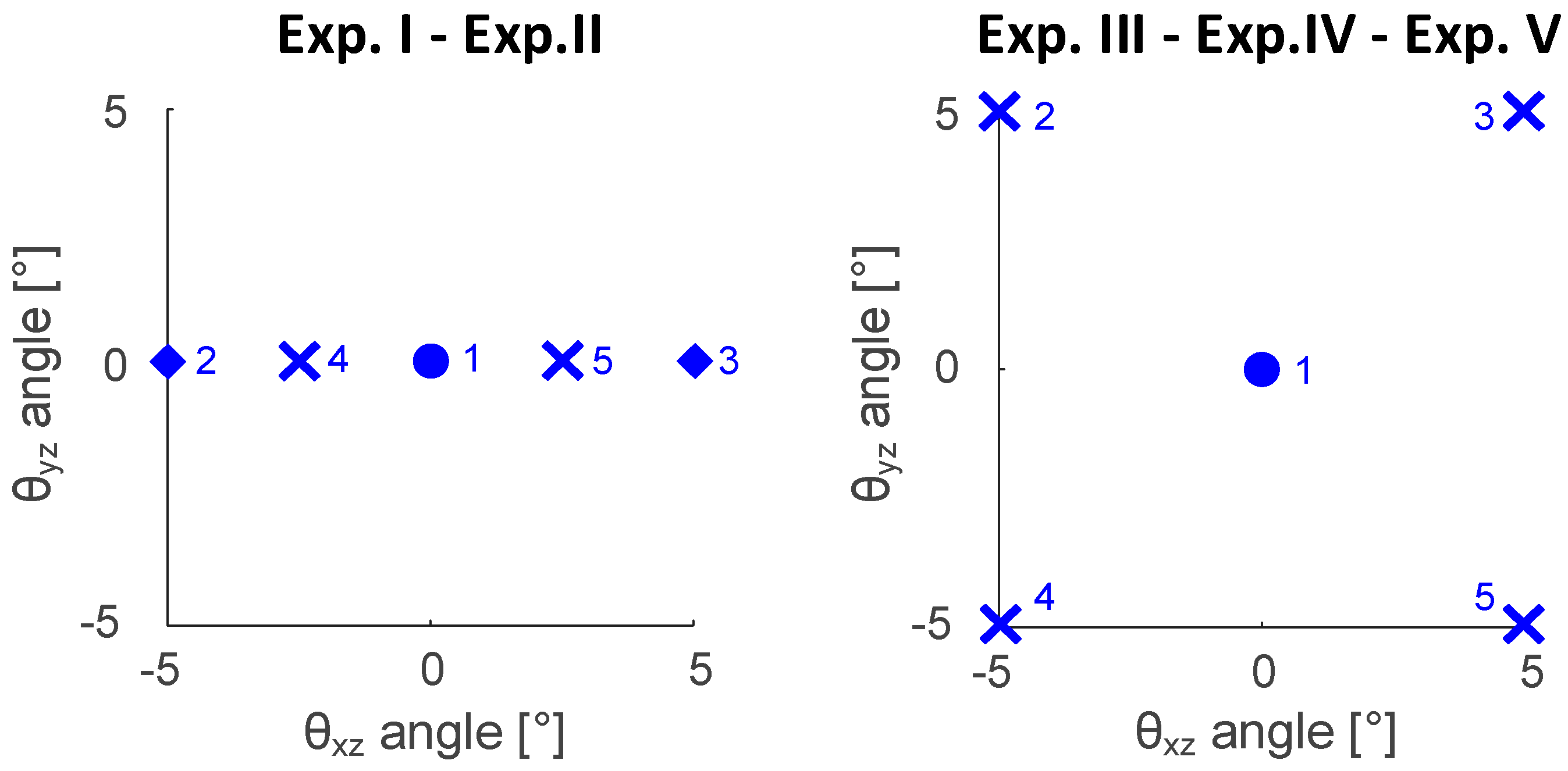
To overcome the B_MC limitation, a new communication channel between the DSPs hosted by “adjacent” FE boards has been established by exploiting the SRIO link. The new topology transfers the baseband samples from the DSPs of one FE to the DSPs on a neighboring FE board. Specifically, as shown in Figure 2 (right panel), the DSPs of FE₁ transfer the baseband partially beamformed samples to the DSPs of FE₂. These DSPs coherently sum such samples with the partially beamformed samples created by FE₂, thus contributing to a 64-channel beamformed image. This operation is repeated until the last installed FE board, FE_N, completes the beamforming addition. Therefore, in this topology, only the last board sends data to the MC board, and a transfer bandwidth B_MC = B_IQ rather than B_MC = N_FE × B_IQ must be sustained. Furthermore, the transmission of final fully beamformed data, rather than of N_FE groups of partially beamformed data, correspondingly reduces the amount of data to be transferred to the MC board. The ring sum operations are performed in pipeline thanks to a special scheduling implementation, which exploits the multi-core architecture of the DSPs, thus no significative delays are introduced. Furthermore, it is worth highlighting that the acquisition task, which is the same in both topology, is handled in parallel to the elaboration chain, so, the ring topology does not affect in any way the TX/RX sequences of the scanner.

3. Experiments

Five HFR experimental tests were performed by using, in each case, both star and ring topologies. In all experiments, a 2-D spiral array probe [41] capable of scanning either a single plane, a bi-plane, or a full volume, was used. Such a probe was obtained by selecting 256 elements from the 1024-element Vermon matrix probe [42].

In addition, 3.7 MHz 4-cycle sinusoidal bursts were used as TX signals. The ULA-OP 256 was programmed to transmit sequences of diverging waves originating from one (DW1), three (DW3), or five (DW5) virtual sources. The position (x, y, z) of each virtual source was defined as follows:

$$\{\begin{array}{c}z=\frac{-\mathsf{\rho }}{\sqrt{1+\mathrm{tg}{\left({\mathsf{\theta }}_{\mathrm{xz}}\right)}^2+\mathrm{tg}{\left({\mathsf{\theta }}_{\mathrm{yz}}\right)}^2}}\\ \mathrm{x}=\mathrm{z} \mathrm{t}\mathrm{g}\left({\mathsf{\theta }}_{\mathrm{xz}}\right)\\ \mathrm{y}=\mathrm{z} \mathrm{t}\mathrm{g}\left({\mathsf{\theta }}_{\mathrm{yz}}\right)\end{array}$$

(6)

where $\mathsf{\rho }$ is the virtual source distance from the center of the array, θ_xz and θ_yz are the projection of the steering angle over the xz and yz planes, respectively.

The FPGA beamformers [40] were configured to reconstruct all the lines of one frame during each RX interval. Therefore, for DW1 sequences the FR was equal to PRF. For DW3 and DW5, in which three and five frames were coherently compounded, the corresponding FR values were calculated by dividing the PRF by three or five, respectively.

Table 2. Table of the experiments performed on star and ring topologies.

	Experiment I	Experiment II	Experiment III	Experiment IV	Experiment V
Mode	DW1 DW3 DW5	DW1 DW3 DW5	DW1   DW5	DW1   DW5	DW1   DW5
Fs [MHz]	39.06			26.04
NCH	128	256
Ndepths	1280			896
NL	96		96 × 2		32 × 30

summarizes the main settings used in the experiments. A depth range of 25 mm (from 5 to 30 mm) was covered in all cases. In experiments I-III such range was obtained through 1280 RF samples (N_depths) at F_S = 39.06 MHz, while in the remaining experiments N_depths was 896 and F_S was 26.04 MHz. In all experiments, N_G was set to 512. N_L represents the number of lines contributing to the final image or volume.

In Experiment I, 128 active elements (i.e., N_FE = 4) contributed to the formation of. 2-D images composed of 96 lines each. These settings allowed us to evaluate the performance achievable when a small number of elements/channels are involved in 2-D HFR imaging.

Experiment II aimed to demonstrate the performance obtainable with a higher number of elements (N_CH = 256). Since 2-D images over the xz-plane were obtained in both Experiment I and Experiment II, the positions of the virtual sources were steered only over the xz-plane (θ_yz = 0° and θ_xz = −5, −2.5, 0, 2.5, 5°), as shown in the left panel of Figure 3, ρ was here 6.28 mm, to ensure a diverging wave opening angle of 60°.

In Experiment III, the 2-D probe was used to perform bi-plane imaging, i.e., the simultaneous creation of two images, each of 96 lines, over planes at rotational angles of 0° and 90°, respectively.

Bi-plane imaging was also performed in Experiment IV, but the computational load was reduced by decreasing the sampling frequency (from 39.06 to 26.04 MHz) and the number (N_depths) of RF samples (from 1280 to 896). This test permitted us to evaluate whether relaxing the requirements on the memories through a reduction of the number of samples could improve the overall system performance.

Experiment V finally considered full 3-D imaging of a small volume scanned through 32 × 30 lines. In this experiment, the sampling frequency was the same as that used in Experiment IV.

Since Experiment III, IV, and V aimed at 3-D imaging, the DW5 imaging sequences exploited diverging waves steered both over the xz and yz planes, as shown in the right panel of Figure 3, while ρ was maintained at 6.28 mm. In these experiments, the DW3 scan sequence was not implemented, because the transmission of three diverging waves does not produce a symmetrical sonification of the volumetric region of interest, as necessary to ensure the same compound image quality in both lateral directions of the volume.

The maximum imaging frame/volume rate achievable in real-time, FR_MAX, was evaluated as follows: the PRF was increased, with a minimum step of 50 Hz in Experiments I–IV, and 10 Hz in Experiment V, by checking, at each step, that the scanner continued to work correctly. Specific debugging signals were appropriately set on the most critical sections of the transfer and elaboration chains to verify their correct execution. In addition, other signals were set to highlight possible overflow on the system’s memories. The highest PRF value that produced properly reconstructed images was considered PRF_MAX. The FR_MAX value was then calculated according to the scan sequence and the number of compounded frames.

For each condition corresponding to the achievement of FR_MAX, the corresponding average beamformer output bandwidth (B_BF, here expressed in terms of beamformed samples per second), and the MC bandwidth (B_MC) were measured to establish whether any of them was acting as a bottleneck.

4. Results and Discussion

Table 3. System performance achieved during experiments I–V.

		Exp. I			Exp. II			Exp. III		Exp. IV		Exp. V
	NL × Ndepths NCH	96 × 1280 128			96 × 1280 256			(96 × 2) × 1280 256		(96 × 2) × 896 256		(32 × 30) × 896 256
	Mode	DW1	DW3	DW5	DW1	DW3	DW5	DW1	DW5	DW1	DW5	DW1	DW5
STAR	FRMAX [Hz]	1500	1500	1000	750	733	740	360	370	360	370	75	74
	BBF [MSPS]	184	553	614	92	270	455	88	455	65	318	65	318
	BMC [GB/s]	1.77	1.77	1.18	1.77	1.73	1.75	1.70	1.75	1.77	1.75	1.77	1.75
RING	FRMAX [Hz]	4200	1700	1020	4400	1667	1000	2200	500	2700	650	510	140
	BBF [MSPS]	516	627	627	541	614	614	541	614	464	568	439	602
	BMC [GB/s]	1.24	0.50	0.30	1.30	0.49	0.29	1.30	0.29	1.59	0.39	1.50	0.41
	FRMAX incr.	+180%	+13%	+2%	+487%	+127%	+35%	+529%	+35%	+620%	+78%	+580%	+89%

summarizes the system performance assessed for the five experiments. The estimated FR_MAX values are bold highlighted. All metrics that correspond to the achievement of the expected maximum limit (bottleneck) are highlighted in orange.

The results show that, compared to the star topology, the ring topology allows the achievement of higher FR_MAX in all cases, with increments up to 620% (see the row at bottom) for DW1 imaging sequences. However, the increments are not homogeneous throughout the experiments. The minimum differences were found when a small number of channels was processed (Experiment I): in this case, the star topology, especially for the DW3 and DW5 imaging sequences, turns out to be almost as efficient as the ring one. The results also confirm that the FR_MAX differences are, in general, significantly reduced when compounding is applied.

These results can be explained as follows. As suggested by the orange-highlighted values, for the star configuration, B_MC is, in most cases, close to the upper limit (≈1.8 GB/s), while the beamformer output rate is much lower than the achievable B_BF value (≈630 MSPS). This means that, in general, the bottleneck was represented by the rate of the SRIO link between the FE boards and the MC board, rather than by the beamformer. Conversely, for the ring configuration, B_BF is always closer to (and B_MC farther from) the upper limit, especially when compounding was applied. This means that the bottleneck was not related to the rate of the SRIO link anymore, i.e., FR_MAX could be increased up to the value permitted by the beamforming rate. Only in the tests of Experiment I that involved compounding (DW3 and DW5), B_BF achieved values close to 630 MSPS for both topologies: correspondingly, the frame rates turned out to be similar, especially in DW5 mode.

It is worth noting that, in the ring topology, for all DW1 cases, both B_MC and B_BF are lower than the theoretical upper limits. This means that the bottleneck is elsewhere. Although this limit could not be quantitatively and systematically assessed, a reasonable hypothesis is that, for PRF values beyond FR_MAX, the DSP cannot sustain the requested working load.

The comparison between the results of Experiment II and Experiment I confirm that the N_CH increase (from 128 to 256) linearly affects FR_MAX for the star (all values are nearly halved) but not for the ring topology. This is consistent with the observation that a two-fold increase in N_CH corresponds to the doubling of the required B_MC in the star topology, but not in the ring topology.

The results of Experiment III confirm that the performance linearly depends on the number of reconstructed lines. Indeed, doubling the number of lines (up to 192), as needed in bi-plane imaging, resulted in a halved FR_MAX.

The results of Experiment IV highlight that relaxing the requirements on the memories by reducing the number of read/write cycles, does not impact the performance of the star topology, which performs as in Experiment III. Although fewer samples were beamformed, the saturation of B_MC still limited FR_MAX. On the other hand, in the ring topology, reducing the RF samples by 33% and relaxing the requirements on the memories led to a 22% increase in FR_MAX compared to Experiment III.

Finally, Experiment V assessed the system performance for HFR imaging of a small volume composed of 960 lines. The results (Table 3 fifth column) show that, in the star topology, the maximum volume rate, FR_MAX, is ≈75 Hz in both DW1 and DW5 sequences. Here, the bottleneck was the saturation of ${\mathrm{B}}_{\mathrm{MC}}$. The ring topology enabled higher FR_MAX values, up to 510 Hz in DW1 and 140 Hz in DW5 mode, respectively: here, the bottleneck was B_BF.

Figure 4 shows sample images obtained when working at FR_MAX for Experiments I, II, and IV on a cylindrical anechoic cyst phantom (Model 040, CIRS Inc., Norfolk, VA, USA). The top images highlight the different qualities obtained when 128 (Exp I—DW1) or 256 (Exp II—DW1) active elements were used. The bottom panels of Figure 4 show B-mode images obtained over two perpendicular planes in Experiment IV—DW5. The images show the cross (left) and longitudinal (right) sections of the cylindrical anechoic cyst.

5. Conclusions

Relevant metrics for the reception stage of an ultrasound system have been identified in Section 2. The results in Table 1 point out that the most critical issues are related to the number of MAC/s operations needed by beamforming, and to the corresponding output data rate. Specifically, for the HFR imaging modalities, more than 1.3 TMAC/s, and data rates as high as 5000 MB/s can be yielded. Such demanding requirements strongly influence both the hardware and the digital architecture of a scanner. Typically, hardware-based scanners use modular architectures [11,43], in which each module manages part of the channels to fit the real-time constraints. Modularity, anyway, also increases the complexity of the system, and special attention must be taken to efficiently distribute the computational and data transfer loads. If this need is not respected, the benefits can be nullified by the bottlenecks that may occur. For example, for HFR 3-D imaging, the amount of beamformed data can be much higher than the amount of raw data (see the examples 3-D PW 256 and 3-D PW 1024 in Table 1): correspondingly, the overall system performance is easily limited by the communication bus.

For the ULA-OP 256, a representative hardware-based scanner, excessively high PRF values determined system instability while performing real-time high frame rate imaging. This could be due to the available resources and their interconnection topology, which in turn caused beamforming limitations, data transfer bottlenecks, or a DSP computational power bottleneck.

Taking advantage of the ring topology over the star topology allowed overcoming the data transfer bottleneck, obtaining up to 4400 frames/s, and more than 1000 compounded frames/s. This is, to the best of our knowledge, the top level HFR performance achieved by an open scanner in real-time. Experiment V also highlighted the requirements and capabilities of a real-time volumetric imaging system. For a small (960 lines) volume, the ULA-OP 256 enabled a maximum volume rate, FR_MAX, of 510 Hz in DW1 and 140 Hz in DW5 mode, respectively. Such volume rates are high enough for morphological imaging and enable the processing by methods based on contour or speckle tracking algorithms with high temporal resolution. Furthermore, it is worth highlighting that the high sampling frequency (39.06 MHz) used in the experiments are high enough to immediately transfer the results shown in Table 3 to probes operating at up to 9.75 MHz.

The results in Table 3 point out that concerning the new ring topology, the remaining bottleneck is, in most cases, represented by the parallel beamforming output rate. However, for all (DW1) cases, in which both B_MC and B_BF are lower than the achievable limits, the bottleneck is probably related to the DSP’s inability to sustain the requested working load.

The possible drawbacks of this topology can also be highlighted. First, data handling and synchronization are surely more complex with respect to the star configuration, especially when many boards are involved. Furthermore, this topology’s results are convenient only in those cases where the performance of a board acting as a central node is limited by a saturation of input transfer bandwidth. This topology in fact cannot increase the parallelization capabilities of a system but can be useful to solve localized and unbalanced transfer bandwidths that limit the computational capacity of a scanner. In conclusion, the proposed ring topology efficiently increased the overall HFR imaging performance of the ULA-OP 256, and these results move a step towards HFR 3-D imaging in real-time. In the next steps, special attention should be given to techniques that could increase the image quality and reduce the overall computational effort of the system. Since 3-D images may suffer from low contrast, the techniques so far proposed in 2-D imaging to increase contrast and spatial resolution [44,45,46] should be considered for application to 3-D imaging. Furthermore, exciting approaches for an efficient delay calculation [47], compressive sensing [48], machine and deep learning-based techniques, intelligent sub-sampling and frequency domain beamforming [49,50], compressed and adaptive beamforming [51,52] are desirable to increase both 3-D image quality and systems performance, pushing future work to be focused on these techniques.

References

1. Szabo, T.L. Diagnostic Ultrasound Imaging: Inside Out, 2nd ed.; Academic Press: Amsterdam, The Netherland; Boston, MA, USA, 2013; ISBN 978-0-12-396487-8. [Google Scholar]
2. Hoskins, P.R.; Martin, K.; Thrush, A. Diagnostic Ultrasound: Physics and Equipment, 3rd ed.; CRC Press: Boca Raton, FL, USA, 2019; ISBN 978-0-367-19041-5. [Google Scholar]
3. Manes, G.; Tortoli, P.; Andreuccetti, F.; Avitabile, G.; Atzeni, C. Synchronous dynamic focusing for ultrasound imaging. IEEE Trans. Ultrason. Ferroelectr. Freq. Control 1988, 35, 14–21. [Google Scholar] [CrossRef] [PubMed]
4. Pye, S.D.; Wild, S.R.; McDicken, W.N. Adaptive time gain compensation for ultrasonic imaging. Ultrasound Med. Biol. 1992, 18, 205–212. [Google Scholar] [CrossRef]
5. Burger, W.; Burge, M.J. Principles of Digital Image Processing: Core Algorithms; Springer: London, UK, 2009; ISBN 978-1-84800-194-7. [Google Scholar]
6. Montaldo, G.; Tanter, M.; Bercoff, J.; Benech, N.; Fink, M. Coherent plane-wave compounding for very high frame rate ultrasonography and transient elastography. IEEE Trans. Ultrason. Ferroelectr. Freq. Control 2009, 56, 489–506. [Google Scholar] [CrossRef] [PubMed]
7. Lewandowski, M.; Walczak, M.; Witek, B.; Kulesza, P.; Sielewicz, K. Modular & scalable ultrasound platform with GPU processing. In Proceedings of the 2012 IEEE International Ultrasonics Symposium, Dresden, Germany, 7–10 October 2012; pp. 1–4. [Google Scholar]
8. So, H.; Chen, J.; Yiu, B.; Yu, A. Medical ultrasound imaging: To GPU or not to GPU? IEEE Micro 2011, 31, 54–65. [Google Scholar] [CrossRef] [Green Version]
9. Jeong, M.K.; Kwon, S.J.; Park, C.D.; Kim, B.S.; Chang, S.H.; Jang, K.S. Ultrasonic imaging research platform with GPU-based software focusing. In Proceedings of the 2017 IEEE International Ultrasonics Symposium (IUS), Washington, DC, USA, 6–9 September 2017; pp. 1–4. [Google Scholar]
10. Jensen, J.A.; Holten-Lund, H.; Nilsson, R.T.; Hansen, M.; Larsen, U.D.; Domsten, R.P.; Tomov, B.G.; Stuart, M.B.; Nikolov, S.I.; Pihl, M.J.; et al. SARUS: A synthetic aperture real-time ultrasound system. IEEE Trans. Ultrason. Ferroelectr. Freq. Control 2013, 60, 1838–1852. [Google Scholar] [CrossRef] [PubMed] [Green Version]
11. Boni, E.; Bassi, L.; Dallai, A.; Guidi, F.; Meacci, V.; Ramalli, A.; Ricci, S.; Tortoli, P. ULA-OP 256: A 256-Channel open scanner for development and real-time implementation of new ultrasound methods. IEEE Trans. Ultrason. Ferroelectr. Freq. Control 2016, 63, 1488–1495. [Google Scholar] [CrossRef]
12. Smith, P.R.; Cowell, D.M.J.; Raiton, B.; Ky, C.V.; Freear, S. Ultrasound array transmitter architecture with high timing resolution using embedded phase-locked loops. IEEE Trans. Ultrason. Ferroelectr. Freq. Control 2012, 59, 40–49. [Google Scholar] [CrossRef] [Green Version]
13. Hasegawa, H.; Kanai, H. High-frame-rate echocardiography using diverging transmit beams and parallel receive beamforming. J. Med. Ultrason. 2011, 38, 129–140. [Google Scholar] [CrossRef]
14. Poree, J.; Posada, D.; Hodzic, A.; Tournoux, F.; Cloutier, G.; Garcia, D. High-frame-rate echocardiography using coherent compounding with doppler-based motion-compensation. IEEE Trans. Med. Imaging 2016, 35, 1647–1657. [Google Scholar] [CrossRef]
15. Fadnes, S.; Wigen, M.S.; Nyrnes, S.A.; Lovstakken, L. In vivo intracardiac vector flow imaging using phased array transducers for pediatric cardiology. IEEE Trans. Ultrason. Ferroelectr. Freq. Control 2017, 64, 1318–1326. [Google Scholar] [CrossRef] [Green Version]
16. Mallart, R.; Fink, M. Improved imaging rate through simultaneous transmission of several ultrasound beams. In Proceedings of the SPIE San Diego ’92, San Diego, CA, USA, 19 July 1992; Volume 1733, pp. 120–130. [Google Scholar]
17. Tong, L.; Gao, H.; D’hooge, J. Multi-transmit beam forming for fast cardiac imaging-a simulation study. IEEE Trans. Ultrason. Ferroelectr. Freq. Control 2013, 60, 1719–1731. [Google Scholar] [CrossRef] [PubMed]
18. Tong, L.; Ramalli, A.; Jasaityte, R.; Tortoli, P.; D’hooge, J. Multi-transmit beam forming for fast cardiac imaging: Experimental validation and in vivo application. IEEE Trans. Med. Imaging 2014, 33, 1205–1219. [Google Scholar] [CrossRef] [PubMed]
19. Ekroll, I.K.; Swillens, A.; Segers, P.; Dahl, T.; Torp, H.; Lovstakken, L. Simultaneous quantification of flow and tissue velocities based on multi-angle plane wave imaging. IEEE Trans. Ultrason. Ferroelectr. Freq. Control 2013, 60, 727–738. [Google Scholar] [CrossRef] [PubMed]
20. Yiu, B.Y.S.; Yu, A.C.H. High-frame-rate ultrasound color-encoded speckle imaging of complex flow dynamics. Ultrasound Med. Biol. 2013, 39, 1015–1025. [Google Scholar] [CrossRef] [PubMed]
21. Tanter, M.; Fink, M. Ultrafast imaging in biomedical ultrasound. IEEE Trans. Ultrason. Ferroelectr. Freq. Control 2014, 61, 102–119. [Google Scholar] [CrossRef]
22. Jensen, J.A.; Nikolov, S.I.; Yu, A.C.H.; Garcia, D. Ultrasound vector flow imaging—Part II: Parallel systems. IEEE Trans. Ultrason. Ferroelectr. Freq. Control 2016, 63, 1722–1732. [Google Scholar] [CrossRef] [Green Version]
23. Posada, D.; Porée, J.; Pellissier, A.; Chayer, B.; Tournoux, F.; Cloutier, G.; Garcia, D. Staggered multiple-prf ultrafast color doppler. IEEE Trans. Med. Imaging 2016, 35, 1510–1521. [Google Scholar] [CrossRef]
24. Faurie, J.; Baudet, M.; Assi, K.C.; Auger, D.; Gilbert, G.; Tournoux, F.; Garcia, D. Intracardiac vortex dynamics by high-frame-rate doppler vortography—In vivo comparison with vector flow mapping and 4-D Flow MRI. IEEE Trans. Ultrason. Ferroelectr. Freq. Control 2017, 64, 424–432. [Google Scholar] [CrossRef]
25. Ricci, S.; Ramalli, A.; Bassi, L.; Boni, E.; Tortoli, P. Real-time blood velocity vector measurement over a 2-D region. IEEE Trans. Ultrason. Ferroelectr. Freq. Control 2018, 65, 201–209. [Google Scholar] [CrossRef]
26. Toulemonde, M.; Li, Y.; Lin, S.; Cordonnier, F.; Butler, M.; Duncan, W.C.; Eckersley, R.J.; Sboros, V.; Tang, M.-X. High-frame-rate contrast echocardiography using diverging waves: Initial in vitro and in vivo evaluation. IEEE Trans. Ultrason. Ferroelectr. Freq. Control 2018, 65, 2212–2221. [Google Scholar] [CrossRef] [Green Version]
27. Guidi, F.; Tortoli, P. Real-time high frame rate color flow mapping system. IEEE Trans. Ultrason. Ferroelectr. Freq. Control 2021, 68, 2193–2201. [Google Scholar] [CrossRef] [PubMed]
28. Orlowska, M.; Bézy, S.; Ramalli, A.; Voigt, J.-U.; D’hooge, J. High-Frame-Rate Speckle Tracking For Echocardiographic Stress Testing. Ultrasound Med. Biol. 2022. [Google Scholar] [CrossRef]
29. Provost, J.; Papadacci, C.; Demene, C.; Gennisson, J.L.; Tanter, M.; Pernot, M. 3-D ultrafast doppler imaging applied to the noninvasive mapping of blood vessels in Vivo. IEEE Trans. Ultrason. Ferroelectr. Freq. Control 2015, 62, 1467–1472. [Google Scholar] [CrossRef] [PubMed]
30. Wei, L.; Wahyulaksana, G.; Meijlink, B.; Ramalli, A.; Noothout, E.; Verweij, M.D.; Boni, E.; Kooiman, K.; van der Steen, A.F.W.; Tortoli, P.; et al. High frame rate volumetric imaging of microbubbles using a sparse array and spatial coherence beamforming. IEEE Trans. Ultrason. Ferroelectr. Freq. Control 2021, 68, 3069–3081. [Google Scholar] [CrossRef]
31. Ramalli, A.; Harput, S.; Bezy, S.; Boni, E.; Eckersley, R.J.; Tortoli, P.; D’Hooge, J. High-frame-rate tri-plane echocardiography with spiral arrays: From simulation to real-time implementation. IEEE Trans. Ultrason. Ferroelectr. Freq. Control 2020, 67, 57–69. [Google Scholar] [CrossRef] [PubMed] [Green Version]
32. Harput, S.; Christensen-Jeffries, K.; Ramalli, A.; Brown, J.; Zhu, J.; Zhang, G.; Leow, C.H.; Toulemonde, M.; Boni, E.; Tortoli, P.; et al. 3-D super-resolution ultrasound imaging with a 2-D sparse array. IEEE Trans. Ultrason. Ferroelectr. Freq. Control 2020, 67, 269–277. [Google Scholar] [CrossRef] [PubMed]
33. Savord, B.; Solomon, R. Fully sampled matrix transducer for real time 3D ultrasonic imaging. In Proceedings of the 2003 IEEE Ultrasonics Symposium (IUS), Honolulu, HI, USA, 5–8 October 2003; Volume 1, pp. 945–953. [Google Scholar]
34. Blaak, S.; Yu, Z.; Meijer, G.C.M.; Prins, C.; Lancée, C.T.; Bosch, J.G.; de Jong, N. Design of a micro-beamformer for a 2D piezoelectric ultrasound transducer. In Proceedings of the 2009 IEEE International Ultrasonics Symposium, Roma, Italy, 20–23 September 2009; pp. 1338–1341. [Google Scholar]
35. Matrone, G.; Savoia, A.S.; Terenzi, M.; Caliano, G.; Quaglia, F.; Magenes, G. A volumetric CMUT-based ultrasound imaging system simulator with integrated reception and μ-beamforming electronics models. IEEE Trans. Ultrason. Ferroelectr. Freq. Control 2014, 61, 792–804. [Google Scholar] [CrossRef]
36. Chen, C.; Chen, Z.; Bera, D.; Raghunathan, S.B.; Shabanimotlagh, M.; Noothout, E.; Chang, Z.-Y.; Ponte, J.; Prins, C.; Vos, H.J.; et al. A front-end ASIC with receive sub-array beamforming integrated with a PZT matrix transducer for 3-D transesophageal echocardiography. IEEE J. Solid-State Circuits 2017, 52, 994–1006. [Google Scholar] [CrossRef] [Green Version]
37. Janjic, J.; Tan, M.; Daeichin, V.; Noothout, E.; Chen, C.; Chen, Z.; Chang, Z.-Y.; Beurskens, R.H.S.H.; van Soest, G.; van der Steen, A.F.W.; et al. A 2-D ultrasound transducer with front-end ASIC and low cable count for 3-D forward-looking intravascular imaging: Performance and characterization. IEEE Trans. Ultrason. Ferroelectr. Freq. Control 2018, 65, 1832–1844. [Google Scholar] [CrossRef]
38. Giangrossi, C.; Meacci, V.; Ricci, S.; Matera, R.; Boni, E.; Dallai, A.; Tortoli, P. Virtual real-time for high PRF multiline vector doppler on ULA-OP 256. IEEE Trans. Ultrason. Ferroelectr. Freq. Control 2021, 68, 624–631. [Google Scholar] [CrossRef]
39. Perrot, V.; Polichetti, M.; Varray, F.; Garcia, D. So you think you can DAS? A viewpoint on delay-and-sum beamforming. Ultrasonics 2021, 111, 106309. [Google Scholar] [CrossRef] [PubMed]
40. Boni, E.; Bassi, L.; Dallai, A.; Meacci, V.; Ramalli, A.; Scaringella, M.; Guidi, F.; Ricci, S.; Tortoli, P. Architecture of an ultrasound system for continuous real-time high frame rate imaging. IEEE Trans. Ultrason. Ferroelectr. Freq. Control 2017, 64, 1276–1284. [Google Scholar] [CrossRef] [PubMed]
41. Ramalli, A.; Boni, E.; Savoia, A.S.; Tortoli, P. Density-tapered spiral arrays for ultrasound 3-D imaging. IEEE Trans. Ultrason. Ferroelectr. Freq. Control 2015, 62, 1580–1588. [Google Scholar] [CrossRef] [PubMed]
42. Roux, E.; Ramalli, A.; Liebgott, H.; Cachard, C.; Robini, M.C.; Tortoli, P. Wideband 2-D array design optimization with fabrication constraints for 3-D US imaging. IEEE Trans. Ultrason. Ferroelectr. Freq. Control 2017, 64, 108–125. [Google Scholar] [CrossRef] [PubMed]
43. Song, J.; Zhang, Q.; Zhou, L.; Quan, Z.; Wang, S.; Liu, Z.; Fang, X.; Wu, Y.; Yang, Q.; Yin, H.; et al. Design and implementation of a modular and scalable research platform for ultrasound computed tomography. IEEE Trans. Ultrason. Ferroelectr. Freq. Control 2022, 69, 62–72. [Google Scholar] [CrossRef] [PubMed]
44. Nguyen, N.Q.; Prager, R.W. A spatial coherence approach to minimum variance beamforming for plane-wave compounding. IEEE Trans. Ultrason. Ferroelectr. Freq. Control 2018, 65, 522–534. [Google Scholar] [CrossRef] [Green Version]
45. Matrone, G.; Ramalli, A.; D’hooge, J.; Tortoli, P.; Magenes, G. A comparison of coherence-based beamforming techniques in high-frame-rate ultrasound imaging with multi-line transmission. IEEE Trans. Ultrason. Ferroelectr. Freq. Control 2020, 67, 329–340. [Google Scholar] [CrossRef]
46. Wiacek, A.; González, E.; Bell, M.A.L. CohereNet: A deep learning architecture for ultrasound spatial correlation estimation and coherence-based beamforming. IEEE Trans. Ultrason. Ferroelectr. Freq. Control 2020, 67, 2574–2583. [Google Scholar] [CrossRef]
47. Ibrahim, A.; Hager, P.A.; Bartolini, A.; Angiolini, F.; Arditi, M.; Thiran, J.-P.; Benini, L.; De Micheli, G. Efficient sample delay calculation for 2-d and 3-d ultrasound imaging. IEEE Trans. Biomed. Circuits Syst. 2017, 11, 815–831. [Google Scholar] [CrossRef] [Green Version]
48. Gedalyahu, K.; Tur, R.; Eldar, Y.C. Multichannel sampling of pulse streams at the rate of innovation. IEEE Trans. Signal Process. 2011, 59, 1491–1504. [Google Scholar] [CrossRef] [Green Version]
49. Burshtein, A.; Birk, M.; Chernyakova, T.; Eilam, A.; Kempinski, A.; Eldar, Y.C. Sub-Nyquist sampling and fourier domain beamforming in volumetric ultrasound imaging. IEEE Trans. Ultrason. Ferroelectr. Freq. Control 2016, 63, 703–716. [Google Scholar] [CrossRef] [PubMed] [Green Version]
50. Huijben, I.A.M.; Veeling, B.S.; Janse, K.; Mischi, M.; van Sloun, R.J.G. Learning sub-sampling and signal recovery with applications in ultrasound imaging. IEEE Trans. Med. Imaging 2020, 39, 3955–3966. [Google Scholar] [CrossRef] [PubMed]
51. Luijten, B.; Cohen, R.; de Bruijn, F.J.; Schmeitz, H.A.W.; Mischi, M.; Eldar, Y.C.; van Sloun, R.J.G. Adaptive ultrasound beamforming using deep learning. IEEE Trans. Med. Imaging 2020, 39, 3967–3978. [Google Scholar] [CrossRef] [PubMed]
52. Wagner, N.; Eldar, Y.C.; Friedman, Z. Compressed beamforming in ultrasound imaging. IEEE Trans. Signal Process. 2012, 60, 4643–4657. [Google Scholar] [CrossRef] [Green Version]
Figure 1. Architecture of the research scanner ULA-OP 256. Blocks of 32 echo data are conditioned and partially beamformed by NFE FE boards before being sent to the MC board. Bwr represents the write data transfer bandwidth required to the FE memory to save the 32 channels echo data.
Applsci 12 06562 g001
Figure 2. Schematic diagrams of the star (left panel) and ring data transfer configurations (right panel). In the star topology, all the FE boards send the beamformed lines to the MC board at the same time, so that the BMC requested to sustain the transfer is NFE times higher than the output bandwidth of each FE (BIQ). In the ring topology each FE board sends the data to the neighbor board. The last FE board sends the final beamformed line to the MC board. The BMC requested to sustain the transfer is thus equal to the output bandwidth of a single FE board.
Applsci 12 06562 g002
Figure 3. Virtual source steering angles set during the transmission of diverging waves. Left panel: in Experiments I and II, involving 2-D imaging sequences, the virtual sources were maintained over the imaging xz-plane; only the central source (dot) was used in DW1, two additional lateral virtual sources (diamonds) were used in DW3, and all the five virtual sources (dot, diamonds and crosses) were used in DW5. Right panel: in experiment III IV and V, only the central source (dot) was used for the scan sequence DW1; for the scan sequence DW5, the five sources (dot and crosses) were steered on both the xz and yz angle to ensure an homogeneous insonification of both lateral directions.
Applsci 12 06562 g003
Figure 4. Sample screenshots of the real-time user interface of ULA-OP 256 during phantom investigation. Top panels: sample images obtained with diverging wave transmission (DW1) from 128 (Experiment I) and 256 (Experiment II) elements of the 2-D Vermon probe. Bottom panels: bi-plane (Experiment IV) transverse (left) and longitudinal (right) “compounded” views, simultaneously obtained through the transmission of five diverging waves (DW5).
Applsci 12 06562 g004