
Potential for Energy Utilization of Air Compression Section Using an Open Absorption Refrigeration System

Abstract
:Featured Application
Abstract
1. Introduction
2. Materials and Methods
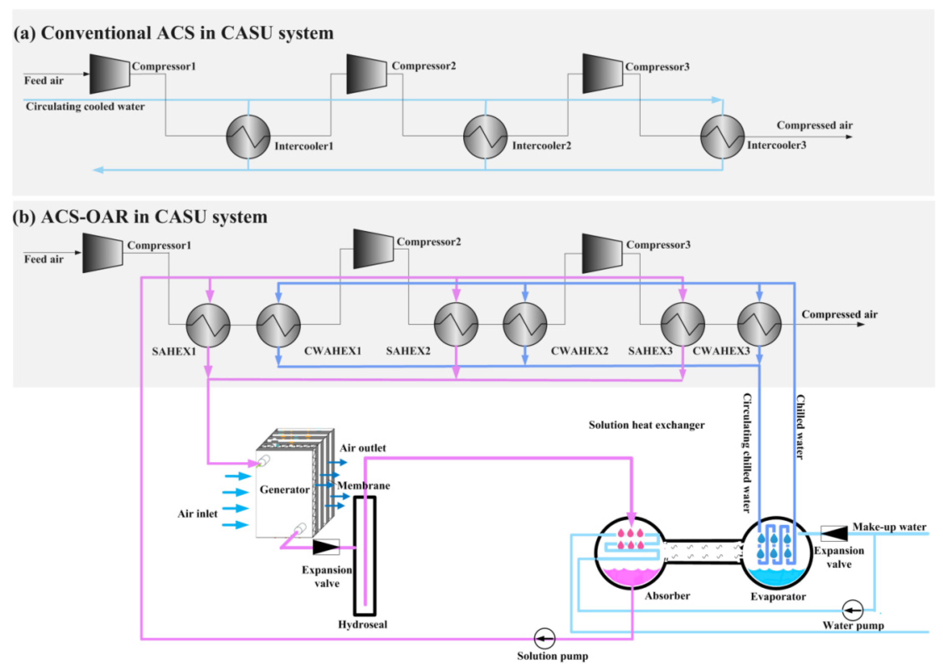
2.1. Conventional Air Compression Section
2.2. Air Compression Section Coupled with OAR System
2.3. Modeling
- The system operates under steady state.
- The heat losses of the devices and pipes are ignored.
- Pressure drops in pipes are neglected.
- Pressures of the absorber and evaporator are the same.
- Solution is saturated at the outlet of the open generator and absorber. Water vapor is saturated at the outlet of the evaporator.
- Heat and mass transfer in the open generator only occur between the liquid and gas phase.
- No condensation occurs in the compression process.
2.3.1. Modeling of the Air Compression Section
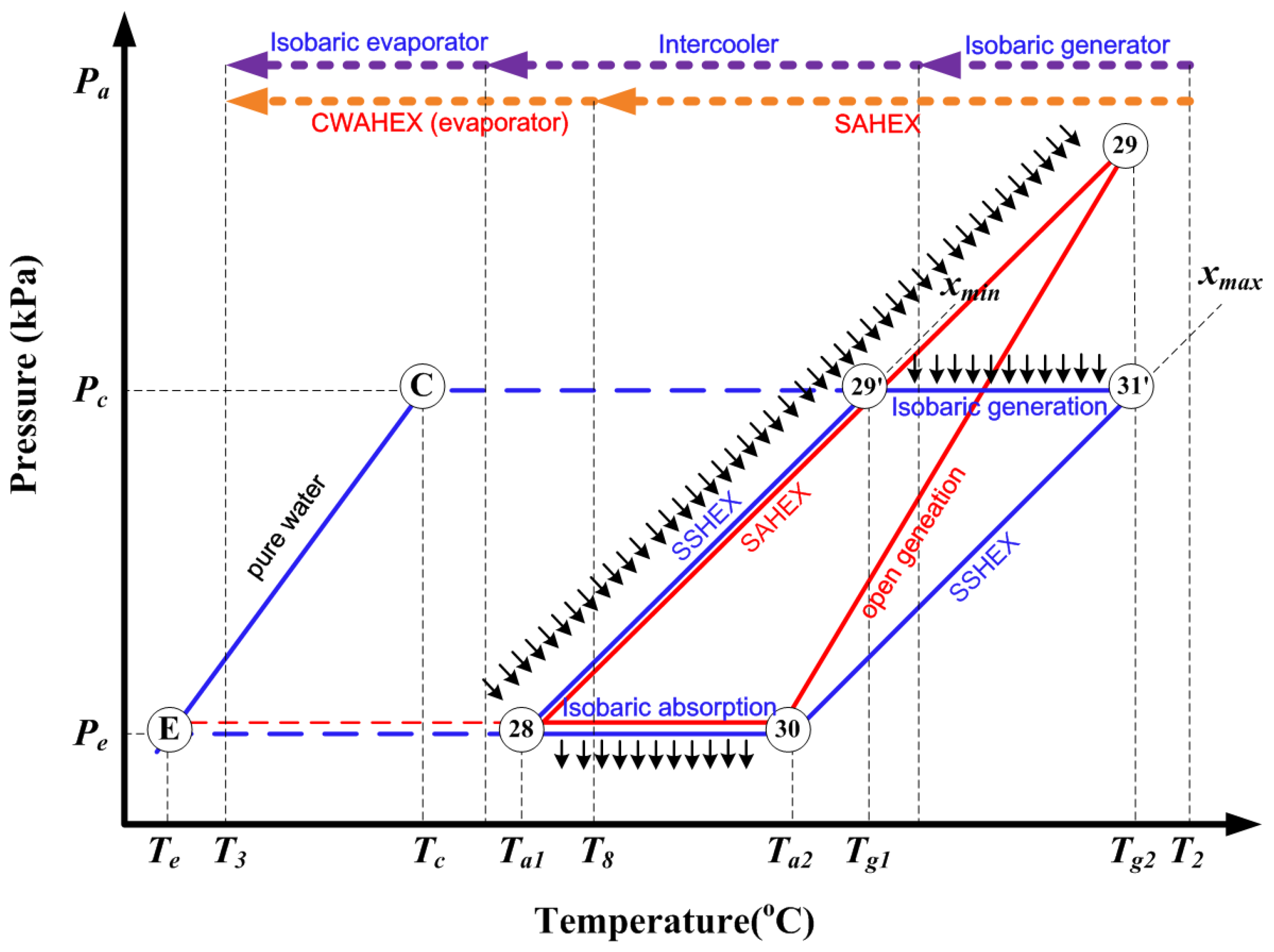
2.3.2. Modeling of OAR System
- (1)
- Evaporator and absorber
- (2)
- SAHEXs and CWHEXs
- (3)
- Open generator
2.3.3. Performance Metrics
2.3.4. Economic Analysis
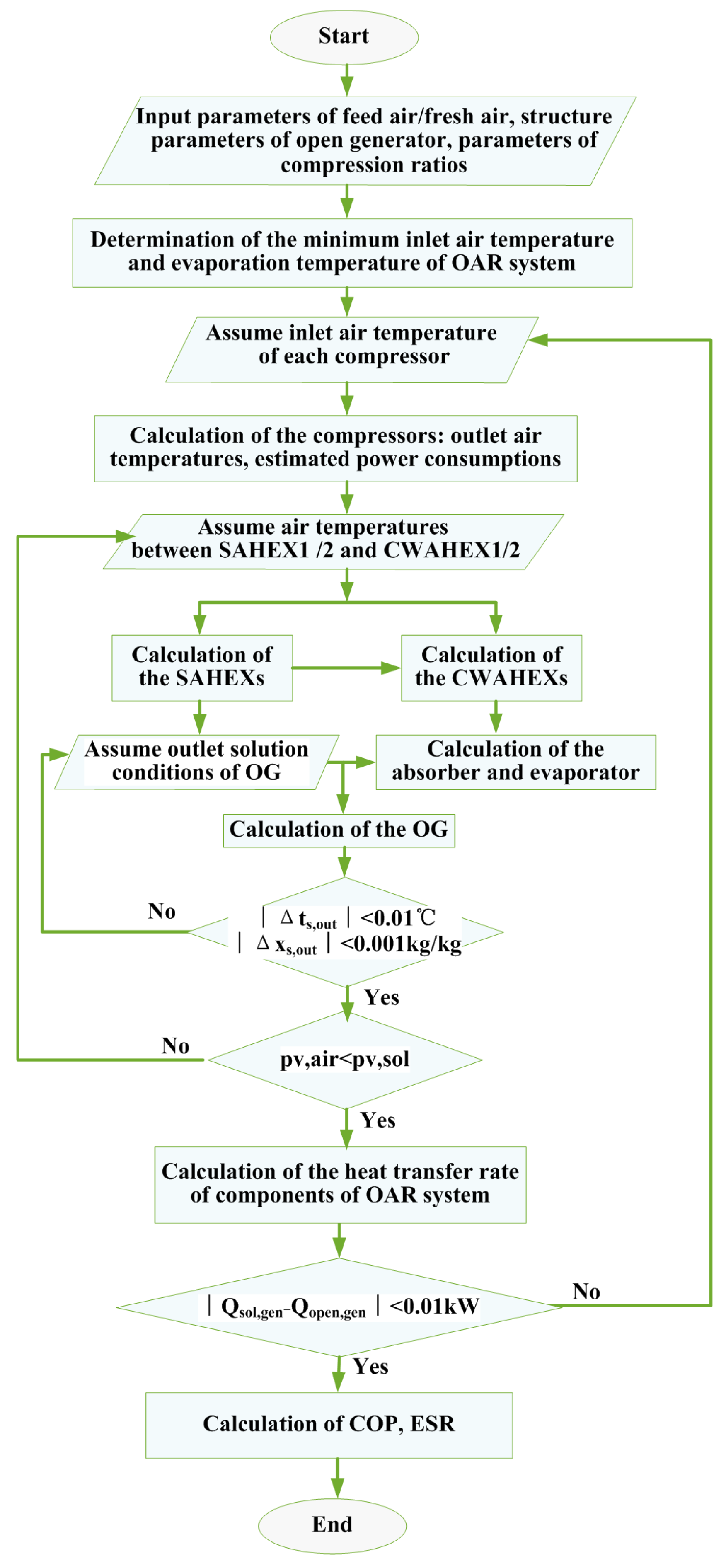
2.3.5. Calculation Procedure
3. Results
3.1. Validation
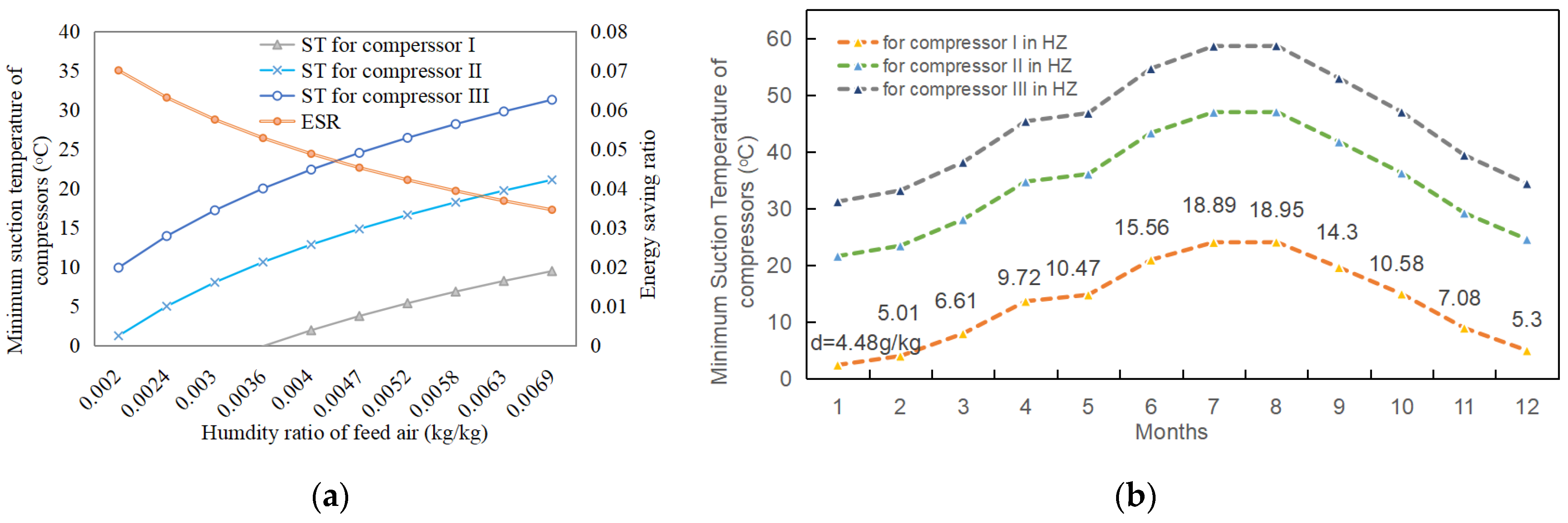
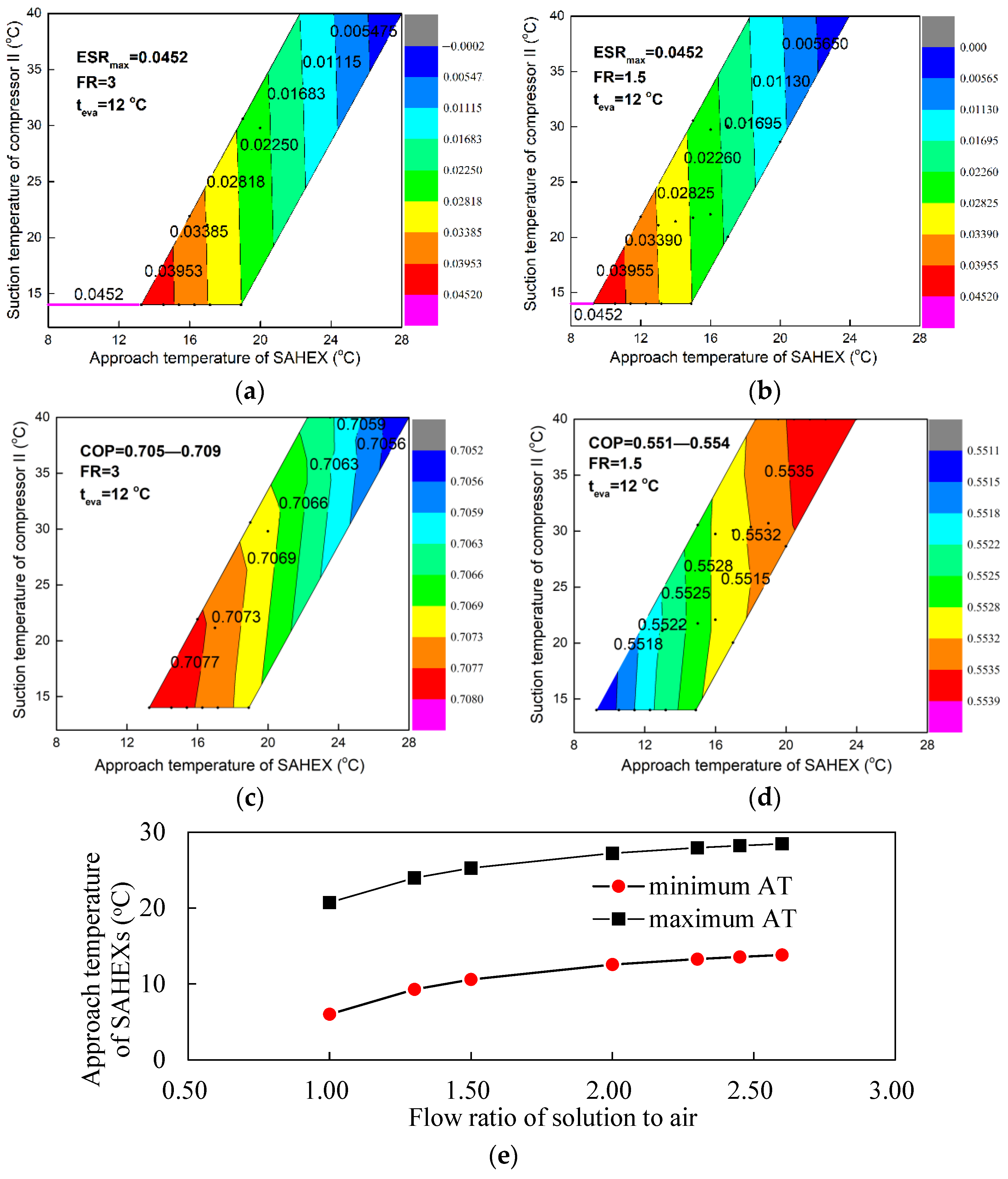
3.2. Optimization of the Suction Temperature
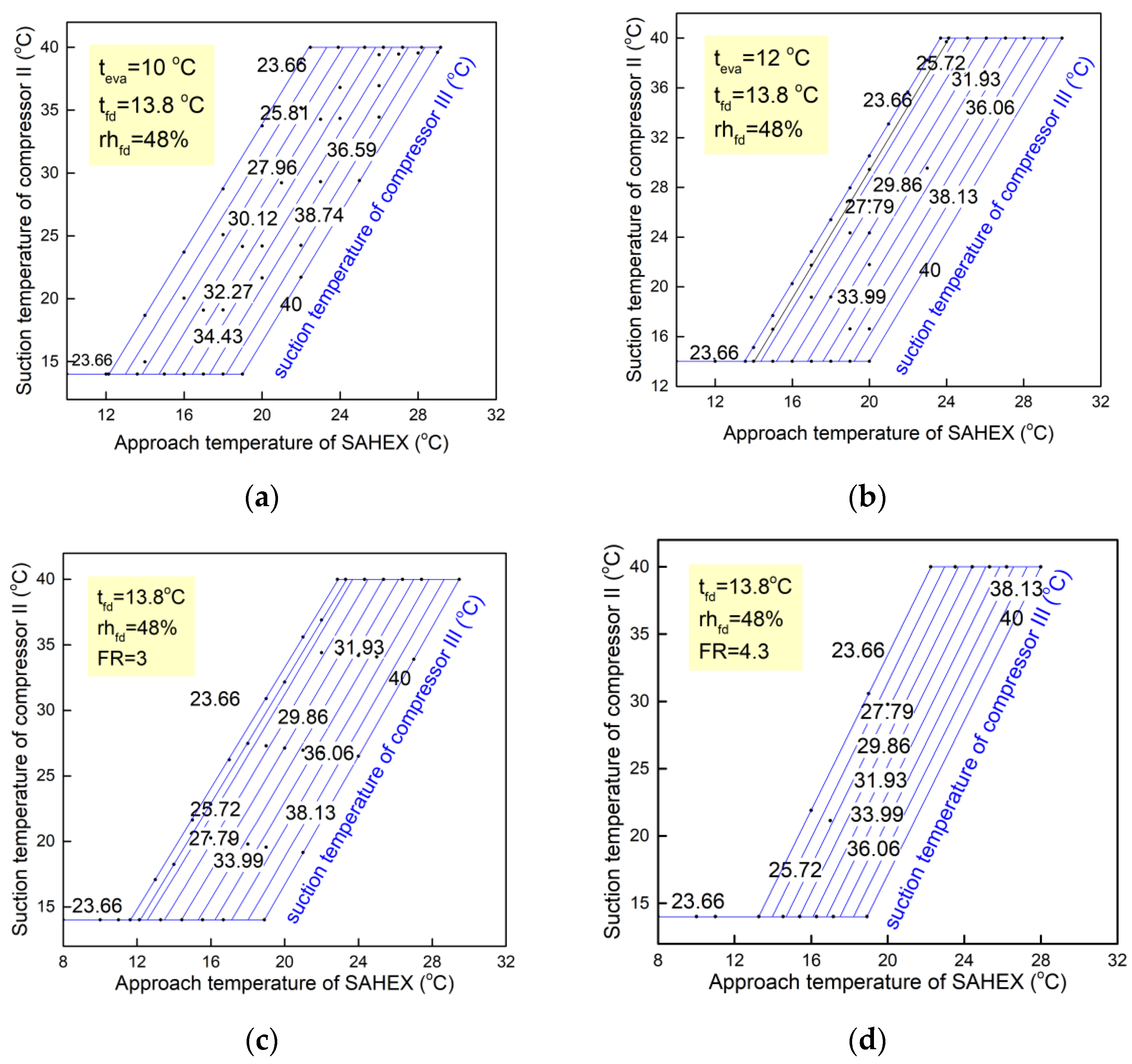
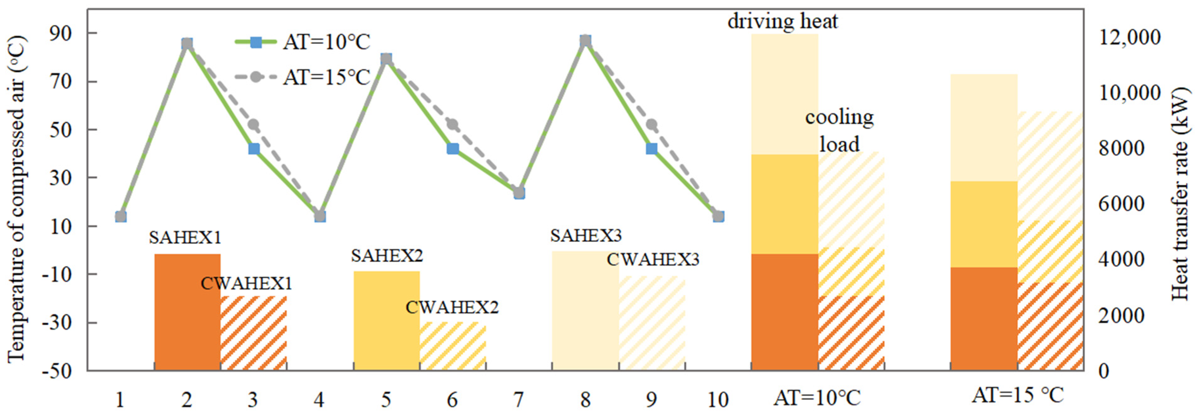
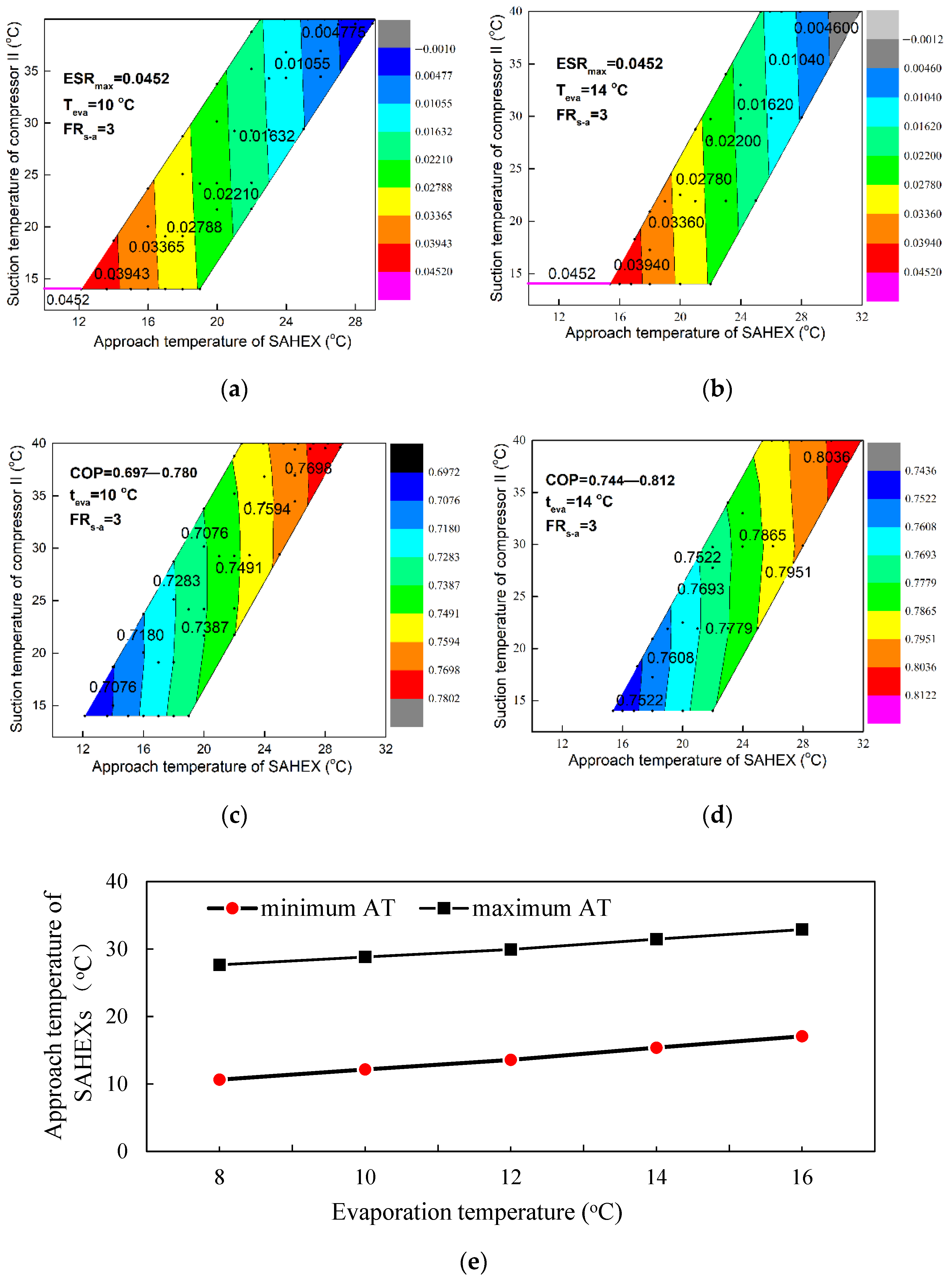
3.3. Parametric Analysis
- (1)
- Internal operating parameters
- (2)
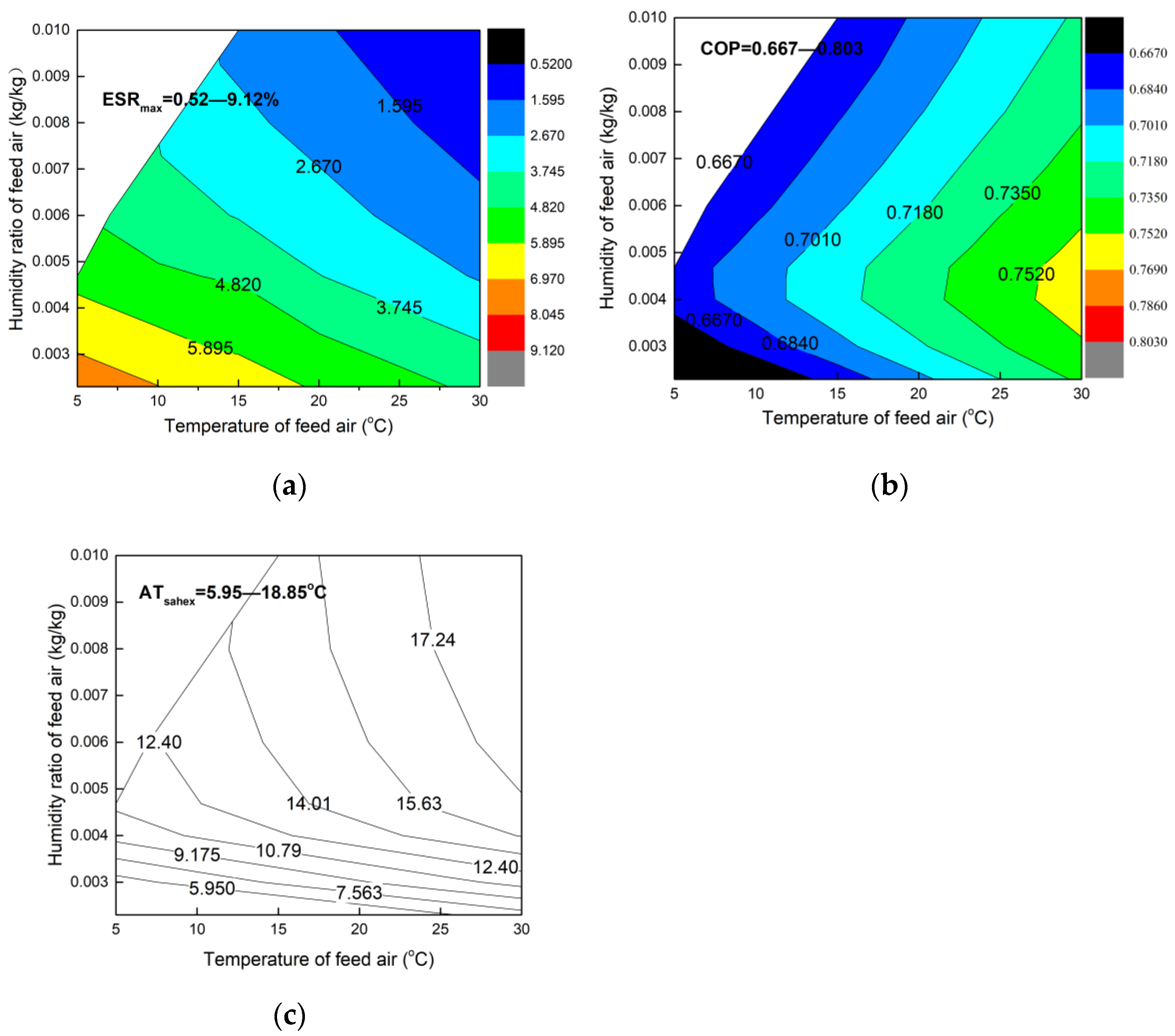
- External operating parameters
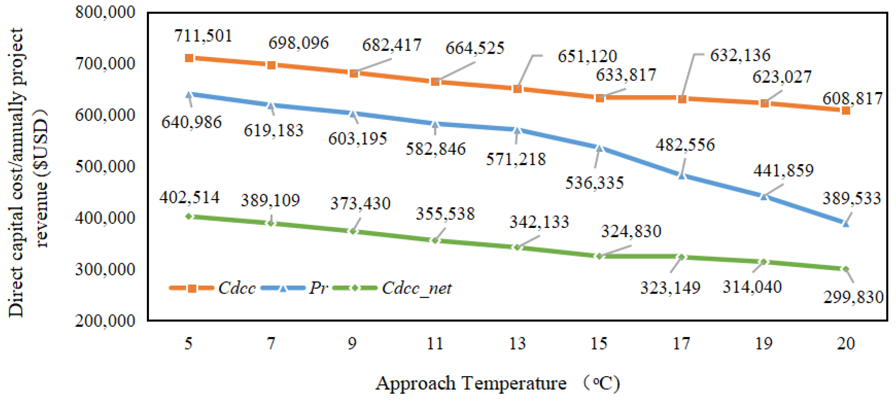
3.4. Economic Analysis
4. Conclusions
- (1)
- The distribution of cooling demand of compressed air, which corresponds to the cooling capacity of the SAHEXs and CWAHEXs of the OAR system, is crucial for the system balance and energy saving performance. Effects of operating parameters, including evaporation temperature, solution-to-air flow ratio, and the approach temperature of the SAHEXs, have been analyzed to illuminate the energy distribution and conversion principle. Ranges of approach temperatures of heat exchangers are optimized under different suction temperatures. The lower limit of approach temperature corresponds to the maximum ESR.
- (2)
- Feed air temperature and humidity ratio have a great impact on the system performance and energy saving potential. ESR ranges from 0.52–8.05%, corresponding to the temperature range of 5–30 °C and humidity range of 0.002–0.010 kg/kg. The annual mean energy saving ratio of the ACS–OAR reaches 4.41% based on the air condition in Beijing. A much higher ESR can be expected by installing a dehydrator before the compressors, as the present ESR is calculated based on a high suction temperature to avoid condensation water in the compressors.
- (3)
- Economic analysis has been conducted to estimate the capital cost, operation cost, and maintenance cost of the OAR system, as well as the net revenue, mainly referring to the electricity saving benefit caused by the coupling of OAR system. The payback period of OAR system is less than one year, and the net project revenue of OAR system during its life cycle reaches USD 5.7 M, showing attractive economic potential.
Author Contributions
Funding
Institutional Review Board Statement
Data Availability Statement
Conflicts of Interest
Nomenclature
| Nomenclature | |
| A | area (m2) |
| C | cost ($) |
| specific heat capacity (J/(kg·K)) | |
| d | absolute humidity of air, kg/kg; |
| dz | length of each segment respectively (m) |
| hydraulic diameter of flow channel | |
| diffusivity coefficient (m2/s) | |
| discounted annual rate | |
| h | enthalpy (kJ/kg) |
| i | sequence of the element indices |
| K | overall mass transfer coefficient (kg/(m2·s)) |
| air side mass transfer coefficient (kg/(m2·s)) | |
| permeability of the membrane (kg/(m·s)) | |
| m | mass flow rate (kg/s) |
| P | pressure (kPa) |
| project revenue | |
| water vapor partial pressure (kPa) | |
| Q | heat transfer rate (kW) |
| R | ideal gas constant (J/(mol·K)) |
| compression ratio (%)T temperature (K) | |
| t | temperature (°C) |
| tax rate | |
| U | overall heat transfer coefficient (W/(m2·K)) |
| air side heat transfer coefficient (W/(m2·K)) | |
| solution side heat transfer coefficient (W/(m2·K)) | |
| power consumption (kW) | |
| x | mass fraction of solvent in the solution (%) |
| isentropic efficiency of compressors (%); | |
| heat transfer effectiveness (%) | |
| solution pump efficiency (%) | |
| thermal conductivity of membrane (W/(m·K)) | |
| thickness of membrane (m) | |
| Abbreviations | |
| ACS | air compression section |
| ACT | air-cooling tower |
| AR | absorption refrigerator |
| ASU | air separation unit |
| CAR | close absorption refrigerator |
| CASU | cryogenic air separation unit |
| COP | Coefficient of performance |
| CWAHEX | cooling water-air heat exchanger |
| DPP | dynamic payback period |
| ESR | energy saving ratio |
| electricity purchase price. | |
| LNG | liquefied natural gas |
| NPV | net present value |
| NTU | number of transfer unit |
| ORC | organic Rankine cycle |
| OAR | open absorption refrigerator |
| SAHEX | solution-air heat exchanger |
| VFMD | vacuum fiber membrane dehumidification |
| VCR | vapor compression refrigerator |
| WCT | water-cooling tower |
| WHRR | waste heat recovery ratio |
| working hours of the system | |
References
- Industry Research Report of Industrial Gas in China. Available online: https://www.djyanbao.com/preview/2986401?from=search_list (accessed on 1 January 2022).
- Tong, L.G.; Zhang, A.J.; Li, Y.L.; Yao, L.; Wang, L.; Li, H.; Li, L.; Ding, Y. Exergy and energy analysis of a load regulation method of CVO of air separation unit. Appl. Therm. Eng. 2015, 80, 413–423. [Google Scholar] [CrossRef] [Green Version]
- Singla, R.; Chowdhury, K. Comparisons of thermodynamic and economic performances of cryogenic air separation plants designed for external and internal compression of oxygen. Appl. Therm. Eng. 2019, 160, 114025. [Google Scholar] [CrossRef]
- Pintilie, M.; Erban, A.; Popa, V.; Popa, C.L. Design analysis of low pressure distillation column for cryogenic air separation. IOP Conf. Ser. Mater. Sci. Eng. 2019, 595, 012023. [Google Scholar] [CrossRef]
- Xu, J.H.; Wang, T.; Chen, Q.; Zhang, S.; Tan, J. Performance design of a cryogenic air separation unit for variable working conditions using the lumped parameter model. Front. Mech. Eng. 2020, 15, 19–26. [Google Scholar] [CrossRef]
- Rong, Y.; Zhi, X.; Wang, K.; Zhou, X.; Cheng, X.; Qiu, L.; Chi, X. Approach to the method to utilize the low-grade residual compression heat during the air separation process. Cryog. Technol. 2019, 1, 5–12. [Google Scholar]
- Wu, Y.; Xiang, Y.; Cai, L.; Liu, H.; Liang, Y. Optimization of a novel cryogenic air separation process based on cold energy recovery of LNG with exergoeconomic analysis. J. Clean. Prod. 2020, 275, 123027. [Google Scholar] [CrossRef]
- Ebrahimi, A.; Ziabasharhagh, M. Optimal design and integration of a cryogenic Air Separation Unit (ASU) with Liquefied Natural Gas (LNG) as heat sink, thermodynamic and economic analyses. Energy 2017, 12, 868–875. [Google Scholar] [CrossRef]
- Rong, Y. Design Optimization and Experimental Research of Self-Enhancement Multi-Stage Air Compression Process Driven by Heat Recovery in Air Separation Units. Ph.D. Thesis, Zhejiang University, Hangzhou, China, 2021. [Google Scholar]
- Lou, H.F.; Li, Y.J.; Shao, Z.J. Dynamic processes of cryogenic air separation distillation systems: A review. J. Chem. Eng. Chin. Univ. 2019, 33, 775–785. [Google Scholar]
- Tian, Q.Q. A Study on Modeling Large-Scale Air Separation Units and Low Energy Consumption. Ph.D. Thesis, Huazhong University of Science and Technology, Wuhan, China, 2016. [Google Scholar]
- Saidur, R.; Rahim, N.A.; Hasanuzzaman, M. A review on compressed-air energy use and energy savings. Renew. Sustain. Energy Rev. 2010, 14, 1135–1153. [Google Scholar] [CrossRef]
- Zhu, S.; Zhang, K.; Deng, K. A review of waste heat recovery from the marine engine with highly efficient bottoming power cycles. Renew. Sustain. Energy Rev. 2020, 120, 109611. [Google Scholar] [CrossRef]
- Aneke, M.; Wang, M. Potential for improving the energy efficiency of cryogenic air separation unit (ASU) using binary heat recovery cycles. Appl. Therm. Eng. 2015, 81, 223–331. [Google Scholar] [CrossRef]
- Zhang, T.; Zhang, X.L.; He, Y.L.; Xue, X.D.; Mei, S.W. Thermodynamic analysis of hybrid liquid air energy storage systems based on cascaded storage and effective utilization of compression heat. Appl. Therm. Eng. 2020, 164, 114526. [Google Scholar] [CrossRef]
- Teng, S.Y.; Wang, M.W.; Xi, H.; Wen, S.Q. Energy, exergy, economic (3E) analysis, optimization and comparison of different ORC based CHP systems for waste heat recovery. Case Stud. Therm. Eng. 2021, 28, 101444. [Google Scholar] [CrossRef]
- Yu, H.S.; Eason, J.; Biegler, L.T.; Feng, X.; Gundersen, T. Process optimization and working fluid mixture design for organic Rankine cycles (ORCs) recovering compression heat in oxy-combustion power plants. Energy Convers. Manag. 2018, 175, 132–141. [Google Scholar] [CrossRef]
- Li, Y.; Zhou, P.; Zhuang, Y.; Wu, X.; Liu, Y.; Han, X.; Chen, G. An improved gas leakage model and research on the leakage field strength characteristics of R290 in limited space. Appl. Sci. 2022, 12, 5657. [Google Scholar] [CrossRef]
- Zheng, Z.Y.; Cao, J.Y.; Wu, W.; Michael, K.H.L. Parallel and in-series arrangements of zeotropic dual-pressure Organic Rankine Cycle (ORC) for low-grade waste heat recovery. Energy Rep. 2022, 8, 2630–2645. [Google Scholar] [CrossRef]
- Rong, Y.; Wu, Q.X.; Zhou, X.; Fang, S.; Wang, K.; Qiu, L.; Zhi, X. Research on optimization of self-utilization performance of air compression waste heat in air separation system. CIESC J. 2021, 72, 13–21. [Google Scholar]
- Rong, Y.; Zhi, X.; Wang, K.; Zhou, X.; Cheng, X.; Qiu, L.; Chi, X. Thermoeconomic analysis on a cascade energy utilization system for compression heat in air separation units. Energy Convers. Manag. 2020, 213, 112820. [Google Scholar] [CrossRef]
- Zhou, X.; Rong, Y.; Fang, S.; Wang, K.; Zhi, X.; Qiu, L.; Chi, X. Thermodynamic analysis of an organic Rankine-vapor compression cycle (ORVC) assisted air compression system for cryogenic air separation units. Appl. Therm. Eng. 2021, 189, 116678. [Google Scholar] [CrossRef]
- Mao, J.; Chen, G.; Ren, Z. Thermoelectric cooling materials. Nat. Mater. 2021, 20, 454–461. [Google Scholar] [CrossRef]
- Chen, W.Y.; Shi, X.L.; Zou, J.; Chen, Z.G. Thermoelectric coolers: Progress, Challenges, and Opportunities. Small Methods 2022, 6, 2101235. [Google Scholar] [CrossRef]
- Rahman, S.M.A.; Hachicha, A.A.; Ghenai, C.; Saidur, R.; Said, Z. Performance and life cycle analysis of a novel portable solar thermoelectric refrigerator. Case Stud. Therm. Eng. 2020, 19, 100599. [Google Scholar] [CrossRef]
- Mansour, K.; Qiu, Y.; Hill, C.J.; Soibel, A.; Yang, R.Q. Mid-infrared interband cascade lasers at thermoelectric cooler temperatures. Electron. Lett. 2006, 42, 1034–1036. [Google Scholar] [CrossRef]
- Huang, B.; Shen, Z.G. Performance assessment of annular thermoelectric generators for automobile exhaust waste heat recovery. Energy 2022, 246, 123375. [Google Scholar] [CrossRef]
- Zhu, X.L.; Zhao, J.; Wu, Y.T.; He, X.L.; Jia, H.L. Dehumidification system for air compressor suction end and waste heat utilization of lubricating oil. Build. Energy Effic. 2017, 8, 101–104. [Google Scholar]
- Du, F.J. Study on the Refrigeration and Use of Interstage Gas’s Waste Heat of Nitrogen-Hydrogen Compressor. Ph.D. Thesis, Zhengzhou University, Zhengzhou, China, 2013. [Google Scholar]
- Zhi, X.; Zhou, X.; Rong, Y.; Li, J.F.; Cheng, X.W.; Qiu, L.M. An Air Separation System with Waste Compression Heat Recovery. CN201710995255.X, 23 October 2017. [Google Scholar]
- Wang, R.Z.; Wang, L.W.; Cai, J.; Du, S.; Hu, B.; Pan, Q.W.; Jiang, L.; Xu, Z.Y. Research status and trends on industrial heat pump and network utilization of waste heat. J. Refrig. 2017, 38, 1–10. [Google Scholar] [CrossRef]
- El-Shafei, B.Z.; Ayman, A.A.; Ahmed, M.H. Modeling and simulation of solar-powered liquid desiccant regenerator for open absorption cooling cycle. Sol. Energy 2011, 85, 2977–2986. [Google Scholar]
- Ayman, A.A.; El-shafei, B.Z.; Ahmed, M.H. Performance evaluation of open-cycle solar regenerator using artificial neural network technique. Energy Build. 2011, 43, 454–462. [Google Scholar]
- Ye, B.C.; Wang, Z.; Yan, X.N.; Chen, G.M. Performance analysis of a variable-stage open absorption heat pump combined with a membrane absorber. Energy Convers. Manag. 2019, 184, 290–300. [Google Scholar] [CrossRef]
- Cost Engineering: Equipment Purchase Costs. Available online: https://www.chemengonline.com/cost-engineering-equipment-purchase-costs/ (accessed on 1 January 2019).
- Rahimi, S.; Meratizaman, M.; Monadizadeh, S.; Amidpour, M. Techno-economic analysis of wind turbineePEM (polymer electrolyte membrane) fuel cell hybrid system in standalone area. Energy 2014, 67, 381–387. [Google Scholar] [CrossRef]
- Sayyaadi, H.; Mehrabipour, R. Efficiency enhancement of a gas turbine cycle using an optimized tubular recuperative heat exchanger. Energy 2012, 38, 362–369. [Google Scholar] [CrossRef]
- Wei, Z.; Zhang, B.; Wu, S.; Chen, Q.; Tsatsaronis, G. Energy-use analysis and evaluation of distillation systems through avoidable exergy destruction and investment costs. Energy 2012, 42, 424–430. [Google Scholar] [CrossRef]


| Parameters | Triple-Stage |
|---|---|
| Components of feed air | Nitrogen 0.7812; Oxygen 0.2095; Argon 0.0093 |
| Feed air mass flow rate (kg/h) | 340,439.85 |
| Product (kg/h) | |
| Liquid O2 (0.3 MPa, −183 °C) | 2992.78 |
| Gas O2 (2.82 MPa, 20 °C) | 71,381.73 |
| Liquid N2 (0.6 MPa, −189.3 °C) | 2499.67 |
| N2 (0.524 MPa, 20 °C) | 56,240.97 |
| N2 (0.114 MPa, 20 °C) | 31,245.44 |
| N2 (1 MPa, 40 °C) | 56,242.79 |
| Outlet pressures of compressors (kPa) | |
| Compressor I | 200 |
| Compressor II | 360 |
| Compressor III | 635 |
| Isentropic efficiency of compressors | 85% |
| Pressure drop of each inter and after coolers (kPa) | 8 |
| Outlet temperatures of intercoolers and aftercooler (°C) | |
| Intercooler I | 40 |
| Intercooler II | 40 |
| Aftercooler I | 40 |
| Variables | |
| Inlet air temperature of feed air (°C) | 13.8–25 |
| Inlet air mass fraction of water (kg/kg) | 0.06–0.016 |
| Properties | Unit | Value | |
|---|---|---|---|
| Membrane thickness | θm | μm | 60 |
| Membrane porosity | ε | % | 75 |
| Membrane pore diameter | dp | μm | 1.0 |
| Tortuosity factor | χ | (2 − ε)2/ε | |
| Membrane thermal conductivity | λ | W/(m·K) | 0.25 |
| Channel Length | L | mm | 200 |
| Channel Width | W | mm | 200 |
| Depth of solution channel | θs | mm | 0.16 |
| Depth of moist gas channel | θg | mm | 1 |
| Equation | |
|---|---|
| Absorber | : Material factor LMTD: Mean logarithmic temperature difference : overall heat transfer coefficient |
| Evaporator | |
| Solution heat exchanger | |
| SA-HEX1/2 | |
| CWA-HEX1/2 | |
| Intercooler | |
| Aftercooler | |
| Pumps and blowers | |
| Compressors | |
| Expansion valves | |
| Air-cooling tower Water-cooling tower | H: Height of the column; d: Diameter of column : Material factor; P: Column mean pressure |
| This Work | Literature [14] | Error | This Work | Literature [32] | Error | ||
|---|---|---|---|---|---|---|---|
| Temperature at the outlet of compressor I (°C) | 109 | 106.3 | 0.025 | Generation heat (kW) | 13,214 | 12,732 | 0.036 |
| Pressure at the outlet of compressor I (kPa) | 198 | 200.6 | −0.013 | Evaporation heat (kW) | 9102 | 8966 | 0.015 |
| Temperature at the outlet of compressor II (°C) | 107 | 104.9 | 0.019 | Absorption heat (kW) | 11,605 | 11,033 | 0.049 |
| Pressure at the outlet of compressor II (kPa) | 346 | 360 | −0.038 | Mass concentration of strong solution | 51.22% | 50.66% | 0.011 |
| Temperature at the outlet of compressor III (°C) | 113 | 109.7 | 0.039 | Outlet temperature of strong solution (°C) | 40.6 | 39.26 | 0.033 |
| Pressure at the outlet of compressor III (kPa) | 635 | 635 | 0 | ||||
| Power consumption of compressors (kW/kg) | 222 | 216 | 0.027 |
| Parameters | Values |
|---|---|
| Life cycle of the system | 25 year |
| Annual working hours | 8000 h |
| Average electricity price | 0.09 USD/kWh |
| Interest rate IR | 8% |
| Discounted rate DR | 2.5% |
| Tax rate | 25% |
| Month | T (°C) | RH (%) | D (kg/kg) | Original Electricity Consumption (kW) | ATsahex = 5 | 7 | 9 | 11 | 13 | 15 | 17 | 19 | 20 |
|---|---|---|---|---|---|---|---|---|---|---|---|---|---|
| ESR (%) | |||||||||||||
| 1 | −1.7 | 0.3 | 0.0001 | 19,872 | 7.01 | 6.84 | 6.49 | 6.12 | 5.85 | 5.34 | 4.61 | 4.87 | 4.49 |
| 2 | −0.7 | 0.39 | 0.0014 | 19,887 | 6.16 | 6.07 | 5.94 | 5.53 | 5.27 | 5.17 | 4.48 | 4.77 | 4.45 |
| 3 | 9.7 | 0.31 | 0.0023 | 20,116 | 5.87 | 5.24 | 5.16 | 5.08 | 5 | 4.72 | 4.14 | 4.56 | 3.27 |
| 4 | 14.7 | 0.43 | 0.0045 | 20,186 | 4.96 | 4.96 | 4.96 | 4.96 | 4.96 | 4.44 | 3.81 | 3.18 | 2.87 |
| 5 | 22.3 | 0.38 | 0.0063 | 20,325 | 4.01 | 4.01 | 4.01 | 4.01 | 4.01 | 4.01 | 3.77 | 3.16 | 2.85 |
| 6 | 26.3 | 0.51 | 0.0108 | 20,552 | 2.67 | 2.67 | 2.67 | 2.67 | 2.67 | 2.67 | 2.67 | 2.36 | 2.07 |
| 7 | 28 | 0.62 | 0.0147 | 20,780 | 0 | 0 | 0 | 0 | 0 | 0 | 0 | 0 | 0 |
| 8 | 25.9 | 0.60 | 0.0119 | 20,266 | 2.46 | 2.46 | 2.46 | 2.46 | 2.46 | 2.46 | 2.46 | 2.11 | 1.83 |
| 9 | 23.1 | 0.58 | 0.0102 | 20,253 | 2.81 | 2.81 | 2.81 | 2.81 | 2.81 | 2.81 | 2.81 | 2.25 | 1.96 |
| 10 | 13.3 | 0.59 | 0.0056 | 20,126 | 4.38 | 4.38 | 4.38 | 4.38 | 4.38 | 3.97 | 3.35 | 2.73 | 2.42 |
| 11 | 5.8 | 0.52 | 0.0030 | 20,006 | 6.15 | 5.68 | 5.04 | 4.81 | 4.77 | 4.13 | 3.49 | 2.9 | 2.61 |
| 12 | −1.2 | 0.49 | 0.0017 | 19,878 | 6.41 | 6.02 | 5.92 | 5.23 | 5.03 | 4.59 | 4.25 | 3.6 | 3.28 |
| annual average | 4.41 | 4.26 | 4.15 | 4.01 | 3.93 | 3.69 | 3.32 | 3.04 | 2.68 | ||||
| Equipment | Design Parameters | Investment Cost (USD) |
|---|---|---|
| OAR system | 711,501 | |
| SAHEX1 | A = 295.4 m2 | 73,522 |
| SAHEX2 | A = 285.3 m2 | 71,871 |
| SAHEX3 | A = 253.7 m2 | 66,594 |
| CWAHEX1 | A = 198.1 m2 | 56,813 |
| CWAHEX2 | A = 293.1 m2 | 73,148 |
| CWAHEX3 | A = 191 m2 | 55,510 |
| Absorber | A = 502.2 m2 | 104,477 |
| Evaporator | A = 401.5 m2 | 79,991 |
| Open generator | A = 424.3 m2 | 84,642 |
| ACT1 | Diameter = 3.5 m, Height = 3 m | 19,533 |
| Pump | Volume rate = 263.8 m3/h | 16,538 |
| Fan | Volume rate = 38.2 m3/s | 8862 |
| Annual operation, maintenance, and management cost | 71,222 | |
| Conventional cooling system | 308,988 | |
| Intercooler1 | A = 328.69 m2 | 72,978 |
| Intercooler2 | A = 345.17 m2 | 75,557 |
| Intercooler3 | A = 383.09 m2 | 81,361 |
| WCT | Diameter = 2.6 m, Height = 1.8 m | 10,850 |
| ACT1 | Diameter = 3.7 m, Height = 3 m | 19,640 |
| ACT2 | Diameter = 4 m, Height = 3.2 m | 23,300 |
| Pumps | Volume rate = 2844 m3/h | 25,300 |
| Annually project revenue (USD) | 640,986 | |
| NPV (USD) | 5,423,691 (based on Capital cost of OAR) 5,709,802 (based on Net Capital cost of cooling system) | |
| DPP | 1.32 year (based on Capital cost of OAR) 0.75 year (based on Net Capital cost of cooling system) | |
Publisher’s Note: MDPI stays neutral with regard to jurisdictional claims in published maps and institutional affiliations. |
© 2022 by the authors. Licensee MDPI, Basel, Switzerland. This article is an open access article distributed under the terms and conditions of the Creative Commons Attribution (CC BY) license (https://creativecommons.org/licenses/by/4.0/).
Share and Cite
Ye, B.; Sun, S.; Wang, Z. Potential for Energy Utilization of Air Compression Section Using an Open Absorption Refrigeration System. Appl. Sci. 2022, 12, 6373. https://doi.org/10.3390/app12136373
Ye B, Sun S, Wang Z. Potential for Energy Utilization of Air Compression Section Using an Open Absorption Refrigeration System. Applied Sciences. 2022; 12(13):6373. https://doi.org/10.3390/app12136373
Chicago/Turabian StyleYe, Bicui, Shufei Sun, and Zheng Wang. 2022. "Potential for Energy Utilization of Air Compression Section Using an Open Absorption Refrigeration System" Applied Sciences 12, no. 13: 6373. https://doi.org/10.3390/app12136373