
Heuristic Approach for a Combined Transfer Line Balancing and Buffer Allocation Problem Considering Uncertain Demand


Abstract
:Featured Application
Abstract
1. Introduction
2. Literature Review
2.1. Transfer Line Balancing Problem
2.2. Buffer Allocation Problem
2.3. Simultanous Approach to TLBP and BAP
- Line configuration: the number of stations and the number of identical machine tools for each station;
- Station configuration: the selection of fixturing type and machine tool type for each station;
- Operation allocation: the allocation of each operation to a station and its positioning in the machining sequence;
- Buffer allocation: the allocation of the buffer capacities between two stations;
- In order to solve the whole problem, several heuristic principles and evolutionary algorithms were built. A priority-based coding system was designed to make the approach suitable for the application of different kinds of algorithms. Four heuristic principles were proposed to ensure the feasibility of the solutions. In order to obtain the optimal set of solutions, Non-dominated Sorting Genetic Algorithm-II (NSGA-II) and Multi-Objective Particle Swarm Optimization (MOPSO) were introduced and fine-tuned, where the total investment cost and the throughput from simulation-based evaluation were considered as the two objective functions. Finally, an industrial case study was introduced to demonstrate the validity of the proposed approach, where the comparison results showed the benefit of NSGA-II for solving the problem.
2.4. Contribution of the Paper
3. Mathematical Model Development
3.1. Assumptions
- A flexible transfer line produces a single part and consists of at least one station in the series and buffer areas between two consecutive stations;
- Multiple machining features are assigned to a single part and each of them has at least one machining operation which needs to be operated in sequence;
- The operation time of each machining operation is known and there may be precedencies among the machining operations;
- A finite number of buffers can be allocated at the buffer area;
- Each station has one or more machine tools that are identical and use an identical type of fixture device to realize the same set of operations;
- Multiple types of machine tools and fixture devices are available. A single machine tool has the possibility to equip with different fixture devices, and vice versa;
- Three parameters for each type of machine tool are known: the mean time to failures (MTTF), the mean time to repair (MTTR), and the machine tool cost;
- Each fixture device enables access to multiple machining features and a datum system used to locate the part;
- A datum system has its machining features (used to locate the part) that have to be machined before the datum system is used;
- The accessible machining features of each station decide the possible machining operations to be allocated to that station.
3.2. Inputs
3.2.1. Production Information
3.2.2. Manufacturing Information
3.2.3. Station Information
3.2.4. Relationship Information
3.3. Decision Variables
- Configuration Information Array, . The size of the array shows the number of stations. The value of describes the number of machine tools at station . It determines the number of stations in the transfer line and the number of identical machine tools for each station;
- Station Information Array, . The value of is the type of number among the station configurations used at station . It determines the type of fixturing and machine tool for each station;
- Operation Information Matrix, . is an allocation and sequencing matrix with the index that determines the position and sequence of each machining operation inside the transfer line;
- Buffer Allocation Array, , The value of shows the number of buffer capacities between station and station .
3.4. Relations and Constraints
3.4.1. Feature Group-Station Configuration Matrix
3.4.2. Datum Feature–Station Configuration Matrix
3.4.3. Station Constraints
3.4.4. Operation Constraints
3.4.5. Buffer Capacity Constraints
3.4.6. Investment Constraints
3.5. Objective Function
4. Solution Approach
4.1. New Approach Logic Diagram
4.2. New Heuristic Principles
- The bottleneck time of a production line is the maximum cycle time among all the stations. It represents the cycle time of the whole production line. However, in this situation, the solutions may have different levels of investment cost, which may make them incomparable simply through the bottleneck time;
- On the contrary, the deviation of allocation time has a more suitable mechanism in this situation. The deviation of allocation time stands for the deviation between the station cycle time and the mean cycle time at all stations of the production line. It evaluates the intrinsic quality of balancing for a single solution under the current investment cost of the manufacturing resources.
4.3. Pre-Screening Strategy
4.4. Simulation Strategy
4.5. Tuning of Algorithm Parameters
5. Industrial Case Study
6. Discussion
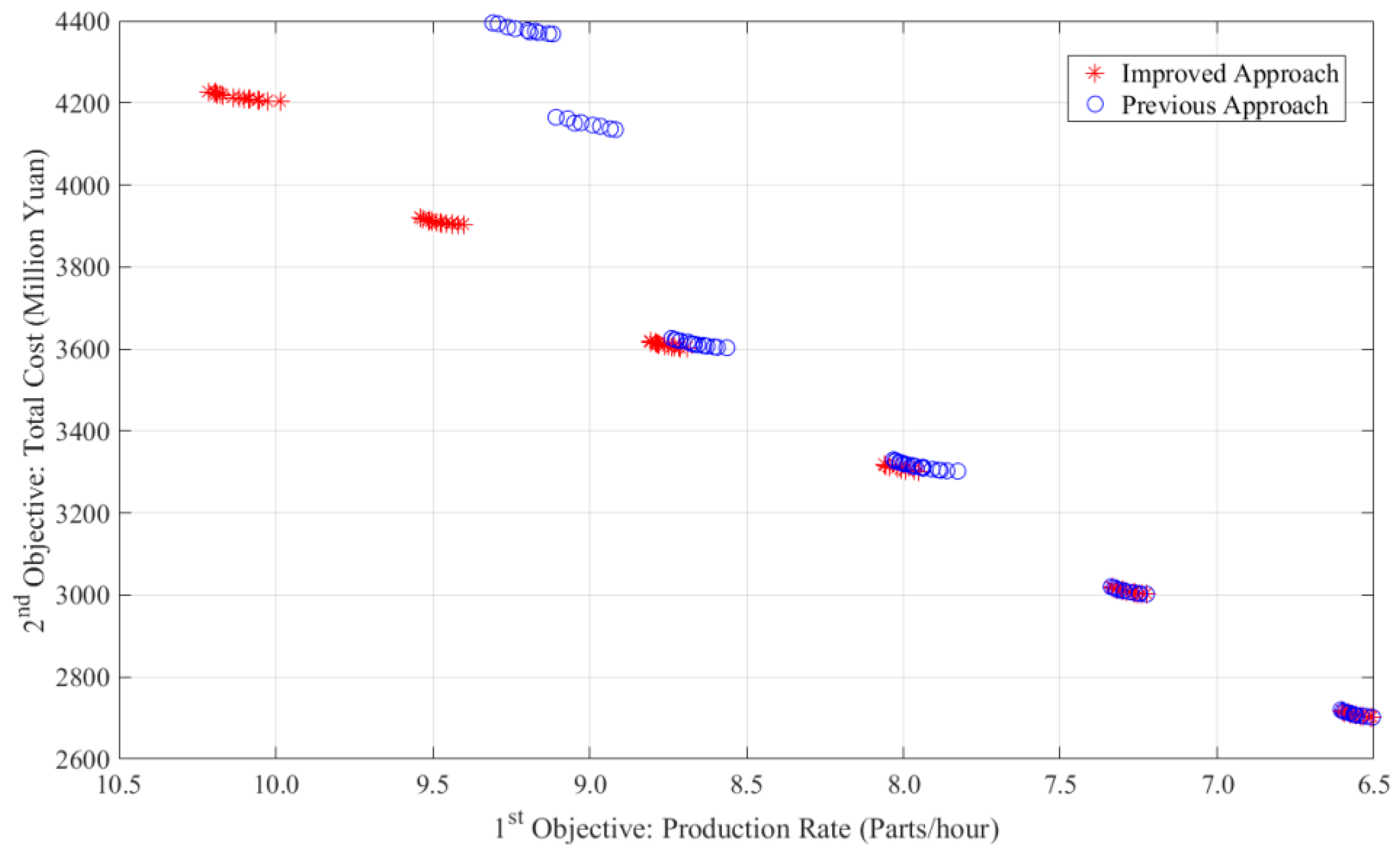
- Solutions in the optimal sets were distributed in groups and could be clustered. Clusters mainly differed with respect to the number and type of machine tools, while the solutions inside a cluster mainly differed with respect to buffer capacity. Of course, the allocation of the operations also influenced the results;
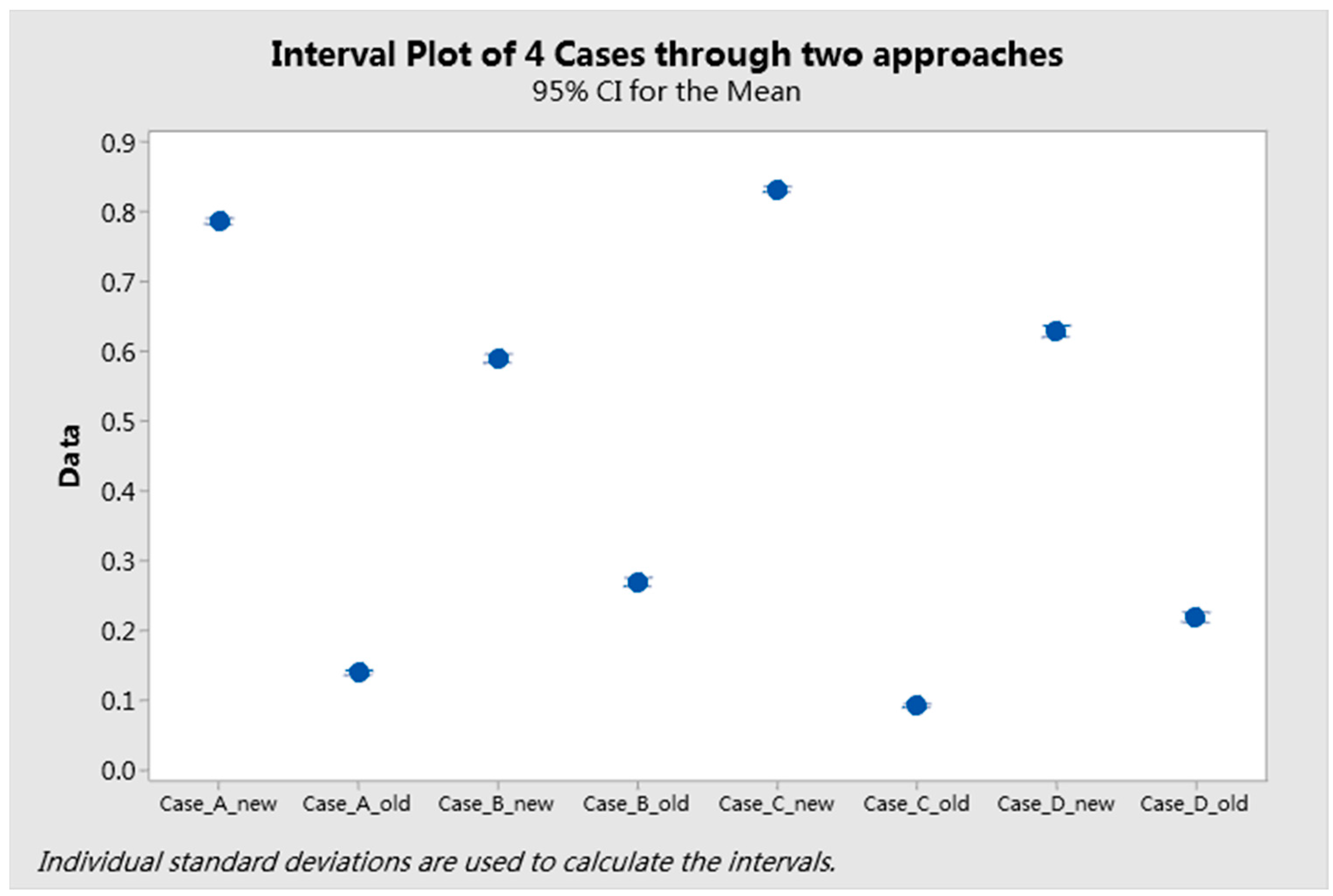
- In the comparison, the overall solutions from the new approach were better than those from the original approach in all four cases;
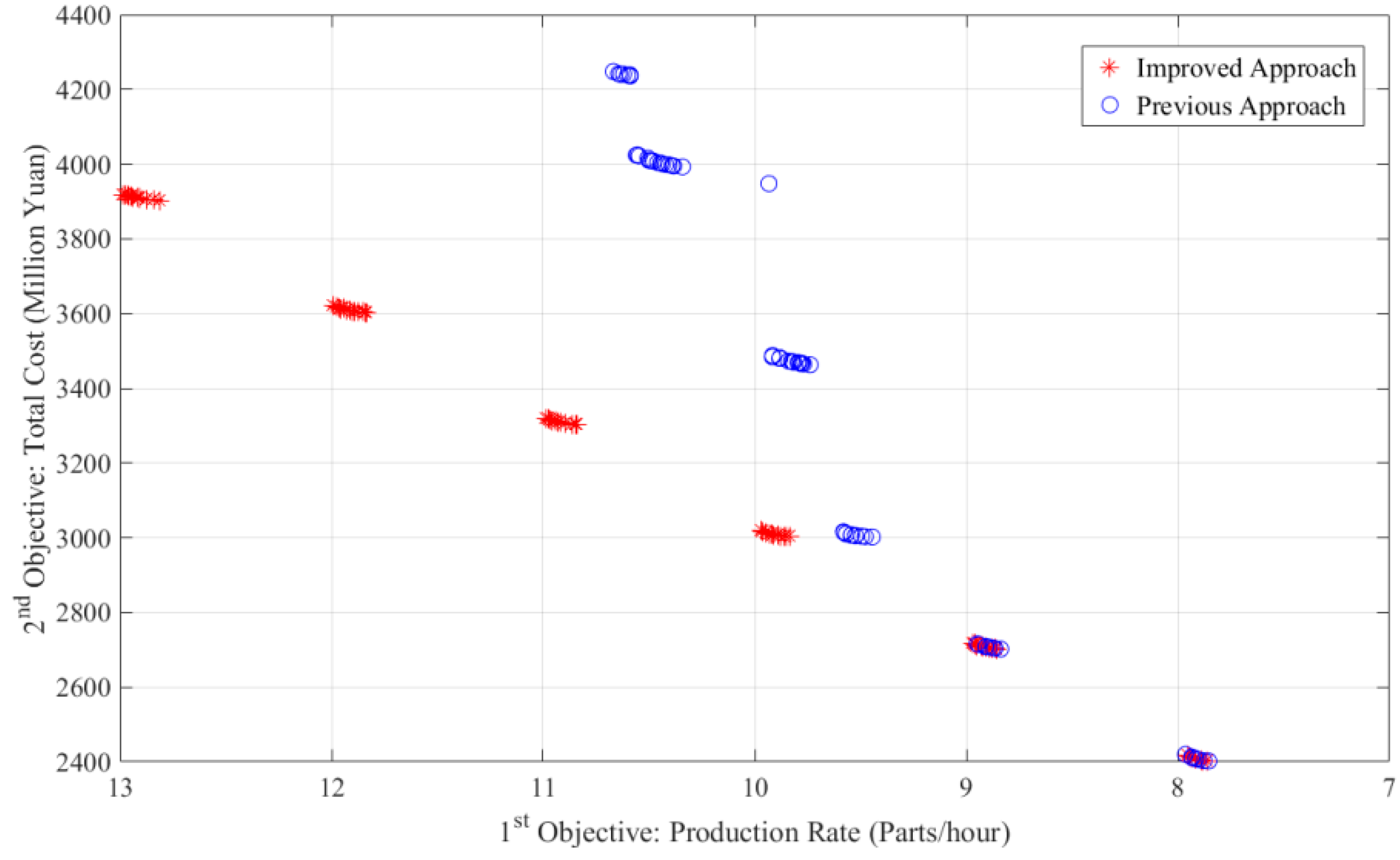
- Considering the details of Case A, there were six clusters in the two optimal sets from both of the algorithms. The first two clusters with a lower production rate from the new algorithm showed slightly better solutions. Starting from the third cluster, the difference between the solutions from the two optimal sets was significantly larger. Considering the third clusters from both of the algorithms, the investment cost of the two clusters was quite similar and around 3.000 Million Yuan, while the production rates of solutions (around 9.9 parts/hour) from the new approach were relatively higher than those from the original approach (around 9.5 parts/hour). Starting from the fourth cluster, it is apparent that the solutions of the cluster from the original approach were fully dominated by those of the corresponding cluster from new approach. This behavior was similar in Case C (Figure A3);
7. Conclusions
Author Contributions
Funding
Institutional Review Board Statement
Data Availability Statement
Acknowledgments
Conflicts of Interest
Appendix A


Appendix B

| Pair | Algorithm Parameters | Response | ||||
|---|---|---|---|---|---|---|
| A | B | C | D | E | NSGA-II | |
| 1 | 1 | 1 | 1 | 1 | 1 | 0.1999 |
| 2 | 1 | 1 | 1 | 1 | 2 | 0.2093 |
| 3 | 1 | 1 | 1 | 1 | 3 | 0.2916 |
| 4 | 1 | 2 | 2 | 2 | 1 | 0.292 |
| 5 | 1 | 2 | 2 | 2 | 2 | 0.2282 |
| 6 | 1 | 2 | 2 | 2 | 3 | 0.5427 |
| 7 | 1 | 3 | 3 | 3 | 1 | 0.5104 |
| 8 | 1 | 3 | 3 | 3 | 2 | 0.5043 |
| 9 | 1 | 3 | 3 | 3 | 3 | 0.5473 |
| 10 | 2 | 1 | 2 | 3 | 1 | 0.3326 |
| 11 | 2 | 1 | 2 | 3 | 2 | 0.4669 |
| 12 | 2 | 1 | 2 | 3 | 3 | 0.343 |
| 13 | 2 | 2 | 3 | 1 | 1 | 0.4473 |
| 14 | 2 | 2 | 3 | 1 | 2 | 0.5425 |
| 15 | 2 | 2 | 3 | 1 | 3 | 0.3336 |
| 16 | 2 | 3 | 1 | 2 | 1 | 0.5696 |
| 17 | 2 | 3 | 1 | 2 | 2 | 0.5799 |
| 18 | 2 | 3 | 1 | 2 | 3 | 0.5799 |
| 19 | 3 | 1 | 3 | 2 | 1 | 0.5169 |
| 20 | 3 | 1 | 3 | 2 | 2 | 0.3894 |
| 21 | 3 | 1 | 3 | 2 | 3 | 0.5214 |
| 22 | 3 | 2 | 1 | 3 | 1 | 0.5586 |
| 23 | 3 | 2 | 1 | 3 | 2 | 0.533 |
| 24 | 3 | 2 | 1 | 3 | 3 | 0.691 |
| 25 | 3 | 3 | 2 | 1 | 1 | 0.5148 |
| 26 | 3 | 3 | 2 | 1 | 2 | 0.4847 |
| 27 | 3 | 3 | 2 | 1 | 3 | 0.5965 |
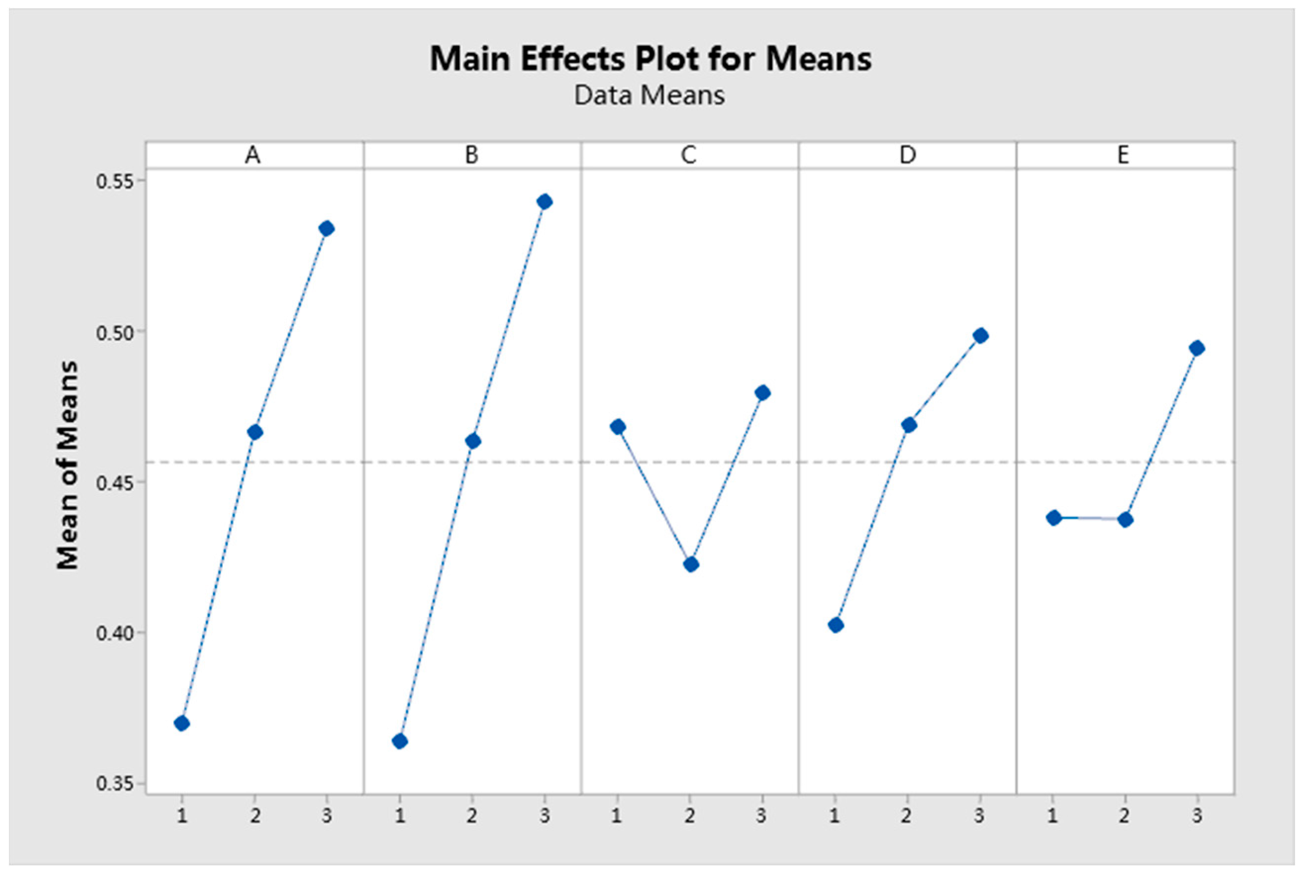
| Level | A | B | C | D | E |
|---|---|---|---|---|---|
| 1 | 0.3695 | 0.3635 | 0.4681 | 0.4023 | 0.4380 |
| 2 | 0.4662 | 0.4632 | 0.4224 | 0.4689 | 0.4376 |
| 3 | 0.5340 | 0.5430 | 0.4793 | 0.4986 | 0.4941 |
| Delta | 0.1645 | 0.1796 | 0.0569 | 0.0963 | 0.0565 |
| Rank | 2 | 1 | 4 | 3 | 5 |
Appendix C
| MT | MTTF [h] | MTTR [h] | Cost [Million CNY] |
|---|---|---|---|
| 1 | 97.353 | 1.388 | 3.0 |
| 2 | 135.135 | 1.646 | 5.3 |
| Possible Station Configuration | 1 | 2 | 3 | 4 | 5 | 6 | 7 | 8 | 9 | 10 | 11 | |
|---|---|---|---|---|---|---|---|---|---|---|---|---|
| Part A | Machine type | 1 | 2 | 1 | 2 | 1 | 2 | 1 | 2 | |||
| Datum system | F0 | F1 | F1 | F1 | F2 | F2 | F3 | F3 | ||||
| Part Orientation | Surface 6 down | Surface 3 down | Surface 6 down | Surface 6 down | Surface 5 down | Surface 5 down | Surface 3 down | Surface 3 down | ||||
| Accessible Surface | 2, 3, 5 | 1, 2, 5 | 2, 3, 5 | 2, 3, 5 | 3, 4, 6 | 3, 4, 6 | 1, 6 | 1, 2, 5 | ||||
| Part B | Machine type | 1 | 1 | 1 | 1 | 2 | 2 | 2 | 2 | 2 | ||
| Datum system | F0 | F1 | F2 | F2 | F0 | F1 | F2 | F2 | F3 | |||
| Part Orientation | Surface 6 down | Surface 3 down | Surface 5 down | Surface 2 down | Surface 6 down | Surface 3 down | Surface 5 down | Surface 2 down | Surface 3 down | |||
| Accessible Surface | 2, 3, 5 | 2, 5, 6 | 3, 4, 6 | 1, 3 | 2, 3, 5 | 2, 5, 6 | 3, 4, 6 | 1, 3 | 1, 2, 5, 6 | |||
| Part C | Machine type | 1 | 1 | 1 | 1 | 2 | 2 | 2 | 2 | 2 | ||
| Datum system | F0 | F1 | F2 | F2 | F0 | F1 | F2 | F2 | F3 | |||
| Part Orientation | Surface 6 down | Surface 3 down | Surface 5 down | Surface 3 down | Surface 6 down | Surface 3 down | Surface 5 down | Surface 3 down | Surface 2 down | |||
| Accessible Surface | 2, 3, 5 | 2, 5, 6 | 1, 4 | 3, 4, 6 | 2, 3, 5 | 2, 5, 6 | 1, 4 | 3, 4, 6 | 1, 2, 5 | |||
| Part D | Machine type | 1 | 1 | 1 | 1 | 1 | 1 | 2 | 2 | 2 | 2 | 2 |
| Datum system | F0 | F1 | F2 | F3 | F2 | F2 | F1 | F2 | F3 | F2 | F2 | |
| Part Orientation | Surface 1 down | Surface 4 down | Surface 1 down | Surface 6 down | Surface 6 down | Surface 4 down | Surface 4 down | Surface 1 down | Surface 6 down | Surface 6 down | Surface 4 down | |
| Accessible Surface | 3, 4 | 1, 2, 6 | 3, 5, 6 | 1, 2 | 2, 3, 4 | 2, 5, 6 | 1, 2, 6 | 3, 5, 6 | 1, 2 | 2, 3, 4 | 2, 5, 6 | |
Appendix D
| Feature Group of Part A | Feature Name | Face | Hole | ||||||||
| Semi-Finish Milling | Finish Milling | Drilling | Gun Drilling | Core Drilling | Rough Boring | Semi-Finish Boring | Finish Boring | Reaming | Tapping | ||
| OFG1 | 10103 | 100.1 | 100.2 | 0 | 0 | 0 | 0 | −10103.1 | −10103.2 | 0 | 0 |
| 10302 | 100.1 | 100.2 | 10302.1 | 0 | 10302.2 | 0 | 0 | 0 | −10302.3 | −10302.4 | |
| 10412 | 100.1 | 100.2 | 10412.1 | 0 | 10412.2 | 0 | 0 | 0 | 0 | −10412.3 | |
| 10603 | 100.1 | 100.2 | 10603.1 | 0 | 0 | 0 | 0 | 0 | 0 | 0 | |
| 10703 | 100.1 | 100.2 | 10703.1 | 0 | 0 | 0 | 0 | 0 | 0 | 0 | |
| 10803 | 100.1 | 100.2 | 10803.1 | 0 | 0 | 0 | 0 | 0 | 0 | 0 | |
| 10902 | 100.1 | 100.2 | 10902.1 | 0 | 0 | 0 | 0 | 0 | 0 | 0 | |
| OFG2 | 20305 | 200 | 0 | 20305.1 | 0 | 0 | 0 | 0 | 0 | 0 | 20305.2 |
| 20417 | 200 | 0 | 20417.1 | 0 | 0 | 0 | 0 | 0 | 0 | 20417.2 | |
| 20501 | 200 | 0 | 0 | 0 | 20501.1 | 0 | 0 | 0 | 20501.2 | 0 | |
| 20601 | 200 | 0 | 20601.1 | 0 | 0 | 0 | 0 | 0 | 0 | 0 | |
| 20703 | 200 | 0 | 20703.1 | 0 | 0 | 0 | 0 | 0 | 0 | 0 | |
| 20801 | 200 | 0 | 20801.1 | 0 | 0 | 0 | 0 | 0 | 0 | 0 | |
| 20901 | 200 | 0 | 20901.1 | 0 | 0 | 0 | 0 | 0 | 20901.2 | 0 | |
| 21001 | 200 | 0 | 21001.1 | 0 | 0 | 0 | 0 | 0 | 0 | 0 | |
| 21101 | 0 | 0 | 21101.1 | 0 | 0 | 0 | 0 | 0 | 21101.2 | 0 | |
| 21202 | 21202.1 | 0 | 0 | 0 | 0 | 0 | 0 | 0 | 0 | 0 | |
| 20104 | 0 | 20104.1 | 0 | 0 | 0 | 20104.2 | 0 | 20104.3 | 0 | 0 | |
| 20208 | 20208.1 | 0 | 0 | 0 | 0 | 0 | 0 | 0 | 0 | 0 | |
| OFG3 | 30402 | 0 | 300.2 | 30402.1 | 0 | 0 | 0 | 0 | 0 | 0 | −30402.2 |
| 30502 | 0 | 0 | 30502.1 | 0 | 0 | 0 | 0 | 0 | 0 | 0 | |
| 30706 | 0 | 300.2 | 30706.1 | 0 | 0 | 0 | 0 | 0 | 0 | −30706.2 | |
| 30901 | 0 | 0 | 30901.1 | 0 | 0 | 0 | 0 | 0 | 0 | 0 | |
| 30604 | 306 | 0 | 30604.1 | 30604.2 | 0 | 0 | 0 | 0 | 0 | 30604.3 | |
| 30802 | 308 | 0 | 30802.1 | 0 | 0 | 0 | 0 | 0 | 0 | 30802.2 | |
| OFG4 | 40302 | 400.1 | 400.2 | 40302.1 | 0 | 0 | 0 | 0 | 0 | 0 | −40302.2 |
| 40407 | 400.1 | 400.2 | 40407.1 | 0 | 0 | 0 | 0 | 0 | 0 | −40407.2 | |
| OFG5 | 50301 | 0 | 0 | 0 | 0 | 50301.1 | 0 | 0 | 0 | 0 | 0 |
| 50408 | 0 | 0 | 50408.1 | 0 | 0 | 0 | 0 | 0 | 0 | 50408.2 | |
| 50507 | 0 | 0 | 50507.1 | 0 | 0 | 0 | 0 | 0 | 0 | 50507.2 | |
| 50702 | 0 | 0 | 50702.1 | 0 | 0 | 0 | 0 | 0 | 50702.2 | 0 | |
| 50801 | 0 | 0 | 50801.1 | 0 | 0 | 0 | 0 | 0 | 50801.2 | 0 | |
| 50903 | 0 | 500.2 | 0 | 0 | 0 | 50903.1 | 50903.2 | −50903.3 | 0 | 0 | |
| OFG6 | 60109 | 601 | 0 | 60109.1 | 0 | 60109.2 | 0 | 0 | 0 | 0 | 60109.3 |
| 60416 | 0 | 600.2 | 60416.1 | 0 | 0 | 0 | 0 | 0 | 0 | −60416.2 | |
| 60502 | 0 | 0 | 60502.1 | 0 | 0 | 0 | 0 | 0 | 0 | 0 | |
| 60806 | 0 | 600.2 | 60806.1 | 0 | 0 | 0 | 0 | 0 | −60806.2 | 0 | |
| FDS1 | F1 | 600.1 | 0 | 60202.1 | 0 | 0 | 0 | 0 | 0 | 60202.2 | 0 |
| FDS2 | F2 | 500.1 | 0 | 50602.1 | 0 | 0 | 0 | 0 | 0 | 50602.2 | 0 |
| FDS3 | F3 | 300.1 | 0 | 30302.1 | 0 | 0 | 0 | 0 | 0 | 30302.2 | 0 |
| SFG1 | S1 | 0 | 0 | 0 | 1502 | 0 | 0 | 0 | 0 | 0 | 0 |
| SFG2 | S2 | 0 | 0 | 31001.1 | 0 | 0 | 0 | 0 | 0 | 0 | 0 |
| SFG3 | S3 | 0 | 0 | 60304.1 | 60304.2 | 0 | 0 | 0 | 0 | 0 | 0 |
| Feature group of Part B | Feature Name | Face | Hole | ||||||||
| Semi-Finish Milling | Finish Milling | Drilling | Gun Drilling | Core Drilling | Rough Boring | Semi-Finish Boring | Finish Boring | Reaming | Tapping | ||
| OFG1 | 10104 | 100.1 | 100.2 | 0 | 0 | 0 | 0 | 10104.1 | −10104.2 | 0 | 0 |
| 10202 | 100.1 | 100.2 | 10202.1 | 0 | 0 | 0 | 0 | 0 | −10202.2 | 0 | |
| 10316 | 100.1 | 100.2 | 10316.1 | 0 | 0 | 0 | 0 | 0 | 0 | 0 | |
| 10402 | 100.1 | 100.2 | 10402.1 | 0 | 0 | 0 | 0 | 0 | 0 | 0 | |
| 10506 | 100.1 | 100.2 | 0 | 10506.1 | 0 | 0 | 0 | 0 | 0 | 0 | |
| 10604 | 100.1 | 100.2 | 10604.1 | 0 | 0 | 0 | 0 | 0 | 0 | 0 | |
| 10701 | 100.1 | 100.2 | 10701.1 | 0 | 0 | 0 | 0 | 0 | 0 | 0 | |
| 10801 | 100.1 | 100.2 | 10801.1 | 0 | 0 | 0 | 0 | 0 | 0 | 0 | |
| OFG2 | 20101 | 200.1 | 200.2 | 0 | 0 | 0 | 20101.1 | 20101.2 | −20101.3 | 0 | 0 |
| 20201 | 200.1 | 200.2 | 0 | 0 | 0 | 0 | 20201.1 | −20201.2 | 0 | 0 | |
| 20301 | 200.1 | 200.2 | 20301.1 | 0 | 0 | 0 | 0 | 0 | −20301.2 | 0 | |
| 20601 | 200.1 | 200.2 | 20601.1 | 0 | 0 | 0 | 0 | 0 | 0 | 0 | |
| 20701 | 200.1 | 200.2 | 20701.1 | 0 | 0 | 0 | 0 | 0 | −20701.2 | 0 | |
| 20801 | 200.1 | 200.2 | 20801.1 | 0 | 0 | 0 | 0 | 0 | 0 | 0 | |
| 21117 | 200.1 | 200.2 | 21117.1 | 0 | 0 | 0 | 0 | 0 | 0 | 0 | |
| 21202 | 200.1 | 200.2 | 21202.1 | 0 | 0 | 0 | 0 | 0 | 0 | 0 | |
| 21301 | 200.1 | 200.2 | 21301.1 | 0 | 0 | 0 | 0 | 0 | 0 | 0 | |
| 21504 | 200.1 | 200.2 | 21504.1 | 0 | 0 | 0 | 0 | 0 | 0 | 0 | |
| 21601 | 200.1 | 200.2 | 21601.1 | 0 | 0 | 0 | 0 | 0 | 0 | 0 | |
| 21701 | 200.1 | 200.2 | 21701.1 | 0 | 0 | 0 | 0 | 0 | −21701.2 | 0 | |
| OFG3 | 30201 | 0 | 0 | 30201.1 | 0 | 0 | 0 | 0 | 0 | 0 | 0 |
| 30405 | 0 | 0 | 30405.1 | 0 | 0 | 0 | 0 | 0 | 0 | 0 | |
| 30701 | 0 | 0 | 30701.1 | 0 | 0 | 0 | 0 | 0 | 0 | 0 | |
| 30801 | 0 | 0 | 30801.1 | 0 | 0 | 0 | 0 | 0 | 0 | 0 | |
| 30901 | 0 | 0 | 30901.1 | 0 | 0 | 0 | 0 | 0 | 0 | 0 | |
| 31008 | 0 | 0 | 31008.1 | 0 | 0 | 0 | 0 | 0 | 0 | 0 | |
| 31201 | 0 | 0 | 31201.1 | 0 | 0 | 0 | 0 | 0 | 0 | 0 | |
| 31308 | 0 | 0 | 31308.1 | 0 | 0 | 0 | 0 | 0 | 0 | 0 | |
| OFG4 | 40102 | 400.1 | 0 | 40102.1 | 0 | 0 | 0 | 0 | 0 | 0 | 0 |
| 40205 | 400.1 | 0 | 40205.1 | 0 | 0 | 0 | 0 | 0 | 0 | 0 | |
| 40510 | 400.1 | 0 | 40510.1 | 0 | 0 | 0 | 0 | 0 | 0 | 0 | |
| 40701 | 400.1 | 0 | 40701.1 | 0 | 0 | 0 | 0 | 0 | 0 | 0 | |
| OFG5 | 50504 | 0 | 0 | 50504.1 | 0 | 0 | 0 | 0 | 0 | 50504.2 | 0 |
| 50708 | 0 | 0 | 50708.1 | 0 | 0 | 0 | 0 | 0 | 0 | 0 | |
| 50807 | 0 | 0 | 50807.1 | 0 | 0 | 0 | 0 | 0 | 0 | 0 | |
| OFG6 | 60210 | 602.1 | 0 | 60210.1 | 0 | 0 | 0 | 0 | 0 | 0 | 0 |
| 60318 | 0 | 600.2 | 60318.1 | 0 | 0 | 0 | 0 | 0 | 0 | 0 | |
| 60403 | 0 | 600.2 | 60403.1 | 0 | 0 | 0 | 0 | 0 | 0 | 0 | |
| 60605 | 0 | 600.2 | 60605.1 | 0 | 0 | 0 | 0 | 0 | 0 | 0 | |
| 60702 | 0 | 0 | 60702.1 | 0 | 0 | 0 | 0 | 0 | 0 | 0 | |
| 60904 | 0 | 0 | 60904.1 | 0 | 0 | 0 | 0 | 0 | 0 | 0 | |
| 61004 | 610.1 | 0 | 61004.1 | 0 | 0 | 0 | 0 | 0 | 0 | 0 | |
| 61108 | 0 | 0 | 0 | 0 | 61108.1 | 0 | 0 | 0 | 0 | 0 | |
| 61205 | 0 | 0 | 0 | 61205.1 | 0 | 0 | 0 | 0 | 0 | 0 | |
| 616 | 616.1 | 616.2 | 0 | 0 | 0 | 0 | 0 | 0 | 0 | 0 | |
| 63000 | 630.1 | 0 | 0 | 0 | 0 | 0 | 0 | 0 | 0 | 0 | |
| FDS1 | F1 | 300.1 | 0 | 0 | 0 | 30104.1 | 0 | 0 | 0 | 30,104.2 | 0 |
| FDS2 | F2 | 500.1 | 0 | 50302.1 | 0 | 50302.2 | 0 | 0 | 0 | 50,302.3 | 0 |
| FDS3 | F3 | 600.1 | 0 | 60102.1 | 0 | 60102.2 | 0 | 0 | 0 | 60,102.3 | 0 |
| SFG1 | S1 | 0 | 0 | 30601 | 20501 | 0 | 0 | 0 | 0 | 0 | 0 |
| Feature group of Part C | Feature Name | Face | Hole | ||||||||
| Semi-Finish Milling | Finish Milling | Drilling | Gun Drilling | Core Drilling | Rough Boring | Semi-Finish Boring | Finish Boring | Reaming | Tapping | ||
| OFG1 | 10104 | 100.1 | 100.2 | 10104.1 | 0 | 10104.2 | −10104.3 | −10104.4 | −10104.5 | 0 | 0 |
| 10202 | 100.1 | 100.2 | 10202.1 | 0 | 10202.2 | 0 | 10202.3 | 0 | 10202.4 | 10202.5 | |
| 10403 | 100.1 | 100.2 | 10403.1 | 0 | 0 | 0 | 0 | 0 | 0 | 0 | |
| 10501 | 100.1 | 100.2 | 0 | 10501.1 | 0 | 0 | 0 | 0 | 0 | 0 | |
| 10616 | 100.1 | 100.2 | 10616.1 | 0 | 10616.2 | 0 | 0 | 0 | 0 | 10616.3 | |
| 10704 | 100.1 | 100.2 | 10704.1 | 0 | 0 | 0 | 0 | 0 | 0 | 0 | |
| 10802 | 100.1 | 100.2 | 10802.1 | 0 | 0 | 0 | 0 | 0 | 0 | 0 | |
| OFG2 | 20119 | 200.1 | 200.2 | 20119.1 | 0 | 0 | 0 | 0 | 0 | 0 | 20119.2 |
| 20201 | 200.1 | 200.2 | 20201.1 | 0 | 0 | 0 | 0 | 0 | 0 | 0 | |
| 20301 | 200.1 | 200.2 | 20301.1 | 0 | 0 | 0 | 0 | 0 | 20301.2 | 0 | |
| 20401 | 200.1 | 200.2 | 0 | 0 | 20401.1 | 0 | 20401.2 | −20401.3 | 0 | 0 | |
| 20501 | 200.1 | 200.2 | 20501.1 | 0 | 0 | 0 | 0 | 0 | −20501.2 | 0 | |
| 20701 | 200.1 | 200.2 | 0 | 0 | −20701.1 | 0 | −20701.2 | 0 | 0 | 0 | |
| 20905 | 200.1 | 200.2 | 20905.1 | 0 | 0 | 0 | 0 | 0 | 0 | 0 | |
| 21002 | 200.1 | 200.2 | 0 | 0 | 0 | 0 | −21002.1 | 0 | 0 | 0 | |
| 21105 | 200.1 | 200.2 | 21105.1 | 0 | 0 | 0 | 0 | 0 | 0 | 0 | |
| 210 | 210.1 | 210.2 | 0 | 0 | 0 | 0 | 0 | 0 | 0 | 0 | |
| OFG3 | 30105 | 0 | 0 | 30105.1 | 0 | 0 | 0 | 0 | 0 | 0 | 30105.2 |
| 30202 | 0 | 0 | 30202.1 | 0 | 0 | 0 | 0 | 0 | 0 | 30202.2 | |
| 30301 | 0 | 0 | 30301.1 | 0 | 0 | 0 | 0 | 0 | 0 | 30301.2 | |
| 30406 | 0 | 0 | 30406.1 | 0 | 0 | 0 | 0 | 0 | 0 | 30406.2 | |
| 30502 | 0 | 0 | 30502.1 | 0 | 0 | 0 | 0 | 0 | 0 | 30502.2 | |
| 30601 | 0 | 0 | 30601.1 | 0 | 0 | 0 | 0 | 0 | 0 | 0 | |
| 30901 | 0 | 0 | 30901.1 | 0 | 0 | 0 | 0 | 0 | 0 | 0 | |
| 31001 | 0 | 0 | 31001.1 | 0 | 0 | 0 | 0 | 0 | 0 | 0 | |
| 30705 | 307.1 | 0 | 30705.1 | 0 | 0 | 0 | 0 | 0 | 0 | 30705.2 | |
| OFG4 | 40102 | 401.1 | 0 | 40102.1 | 0 | 0 | 0 | 0 | 0 | 0 | 40102.2 |
| 40201 | 400.1 | 0 | 40201.1 | 0 | 0 | 0 | 0 | 0 | 0 | 0 | |
| 40302 | 400.1 | 0 | 40302.1 | 0 | 40302.2 | 0 | 0 | 0 | 0 | 40302.3 | |
| 40502 | 400.1 | 0 | 40502.1 | 0 | 0 | 0 | 0 | 0 | 0 | 40502.2 | |
| 40610 | 400.1 | 0 | 40610.1 | 0 | 0 | 0 | 0 | 0 | 0 | 40610.2 | |
| 40704 | 400.1 | 0 | 40704.1 | 0 | 0 | 0 | 0 | 0 | 0 | 40704.2 | |
| 40802 | 400.1 | 0 | 40802.1 | 0 | 0 | 0 | 0 | 0 | 0 | 40802.2 | |
| 40901 | 400.1 | 0 | 40901.1 | 0 | 0 | 0 | 0 | 0 | 0 | 40901.2 | |
| 41001 | 410.1 | 0 | 41001.1 | 0 | 0 | 0 | 0 | 0 | 0 | 41001.2 | |
| OFG5 | 50108 | 0 | 500.2 | 50108.1 | 0 | 0 | 0 | 0 | 0 | 0 | 50108.2 |
| 50401 | 0 | 500.2 | 0 | 50401.1 | 0 | 0 | −50401.2 | 0 | 0 | 0 | |
| 50501 | 0 | 500.2 | 0 | 0 | 0 | 0 | 50501.1 | −50501.2 | 0 | 0 | |
| 50701 | 0 | 500.2 | 0 | 0 | −50701.1 | 0 | −50701.2 | 0 | 0 | 0 | |
| 50601 | 0 | 0 | 50601.1 | 0 | 0 | 0 | 0 | 0 | 0 | 0 | |
| OFG6 | 60119 | 0 | 600.2 | 60119.1 | 0 | 0 | 0 | 0 | 0 | 0 | 60119.2 |
| 60204 | 0 | 600.2 | 60204.1 | 0 | 0 | 0 | 0 | 0 | 0 | 60204.2 | |
| 60308 | 0 | 600.2 | 60308.1 | 0 | 0 | 0 | 0 | 0 | −60308.2 | 0 | |
| 60601 | 0 | 600.2 | 0 | 60601.1 | 0 | 0 | 0 | 0 | 0 | 0 | |
| 60701 | 0 | 600.2 | 60701.1 | 0 | 0 | 0 | 0 | 0 | 0 | 0 | |
| 61104 | 0 | 600.2 | −61104.1 | 0 | 0 | 0 | 0 | 0 | 0 | 0 | |
| 61204 | 0 | 600.2 | −61204.1 | 0 | 0 | 0 | 0 | 0 | 0 | 0 | |
| 61302 | 0 | 600.2 | −61302.1 | 0 | 0 | 0 | 0 | 0 | 0 | 0 | |
| 61401 | 0 | 600.2 | −61401.1 | 0 | 0 | 0 | 0 | 0 | 0 | 0 | |
| 61510 | 0 | 600.2 | −61510.1 | 0 | 0 | 0 | 0 | 0 | 0 | −61510.2 | |
| 60808 | 0 | 0 | 60808.1 | 0 | 0 | 0 | 0 | 0 | 0 | 0 | |
| 604 | 604.1 | 0 | 0 | 0 | 0 | 0 | 0 | 0 | 0 | 0 | |
| 61004 | 610.1 | 0 | −61004.1 | 0 | 0 | 0 | 0 | 0 | 0 | −61004.2 | |
| FDS1 | F1 | 300.1 | 0 | 0 | 0 | 30804.1 | 0 | 0 | 0 | 30804.2 | 0 |
| FDS2 | F2 | 500.1 | 0 | 50302.1 | 0 | 50302.2 | 0 | 0 | 0 | 50302.3 | 0 |
| FDS3 | F3 | 600.1 | 0 | 60502.1 | 0 | 60502.2 | 0 | 0 | 0 | 60502.3 | 0 |
| SFG1 | S1 | 0 | 0 | 10303.1 | 10303.2 | 0 | 0 | 0 | 0 | 0 | 0 |
| Feature group of Part D | Feature Name | Face | Hole | ||||||||
| Semi-Finish Milling | Finish Milling | Drilling | Gun Drilling | Core Drilling | Rough Boring | Semi-Finish Boring | Finish Boring | Reaming | Tapping | ||
| OFG1 | 10102 | 0 | 110.2 | 10102.1 | 0 | 0 | 0 | 0 | 0 | −10102.2 | 0 |
| 10210 | 100.1 | 100.2 | 10210.1 | 0 | 0 | 0 | 0 | 0 | 0 | 0 | |
| 10308 | 0 | 110.2 | 10308.1 | 0 | 0 | 0 | 0 | 0 | 0 | 0 | |
| 10402 | 0 | 110.2 | 10402.1 | 0 | 0 | 0 | 0 | 0 | 0 | 0 | |
| 10604 | 0 | 0 | 10604.1 | 0 | 0 | 0 | 0 | 0 | 0 | 0 | |
| 10907 | 0 | 0 | 0 | 10907.1 | 0 | 0 | 0 | 0 | 0 | 0 | |
| 11201 | 100.1 | 100.2 | 0 | 0 | 0 | 0 | 0 | 0 | 11201.1 | 0 | |
| 11308 | 0 | 0 | 0 | 0 | 0 | 0 | 11308.1 | 0 | 0 | 0 | |
| 11504 | 0 | 110.2 | 0 | 0 | 0 | 0 | 0 | 0 | 11504.1 | 0 | |
| OFG2 | 20102 | 200.1 | 200.2 | 0 | 0 | 0 | 0 | 0 | 0 | 20102.1 | 0 |
| 20118 | 200.1 | 200.2 | 20118.1 | 0 | 0 | 0 | 0 | 0 | 0 | 0 | |
| 20204 | 200.1 | 200.2 | 20204.1 | 0 | 20204.2 | −20204.3 | 20204.4 | 20204.5 | 0 | 0 | |
| 20301 | 200.1 | 200.2 | 20301.1 | 0 | 0 | 0 | 0 | 0 | 0 | 0 | |
| 20404 | 200.1 | 200.2 | 20404.1 | 0 | 0 | 0 | 0 | 0 | 0 | 0 | |
| 20506 | 0 | 0 | 20506.1 | 0 | 0 | 0 | 0 | 0 | 0 | 0 | |
| 20601 | 0 | 0 | 20601.1 | 0 | 0 | 0 | 0 | 0 | 0 | 0 | |
| 20701 | 0 | 0 | 20701.1 | 0 | 0 | 0 | 0 | 0 | 0 | 0 | |
| 20801 | 0 | 0 | 20801.1 | 0 | 0 | 0 | 0 | 0 | 0 | 0 | |
| OFG3 | 30311 | 301.1 | 301.2 | −30311.1 | 0 | 0 | 0 | 0 | 0 | 0 | 0 |
| 30204 | 303.1 | 303.2 | 30204.1 | 0 | 0 | 0 | 0 | 0 | 0 | 0 | |
| 30402 | 303.1 | 303.2 | 30402.1 | 0 | 0 | 0 | 0 | 0 | 0 | 0 | |
| 30503 | 303.1 | 303.2 | 30503.1 | 0 | 30503.2 | 0 | 0 | 0 | 0 | 0 | |
| 30601 | 303.1 | 303.2 | 30601.1 | 0 | 0 | 0 | 0 | 0 | 0 | 0 | |
| 30702 | 303.1 | 303.2 | 30702.1 | 0 | 0 | 0 | 0 | 0 | 0 | 0 | |
| 30801 | 302.1 | 0 | 30801.1 | 0 | 0 | 0 | 0 | 0 | 0 | 0 | |
| OFG4 | 40502 | 405.1 | 0 | 40502.1 | 0 | 0 | 0 | 0 | 0 | 0 | 0 |
| 40610 | 406.1 | 0 | 40610.1 | 0 | 0 | 0 | 0 | 0 | 0 | 0 | |
| 40310 | 403.1 | 0 | 40310.1 | 0 | 0 | 0 | 0 | 0 | 0 | 0 | |
| 40402 | 403.1 | 0 | 40402.1 | 0 | 0 | 0 | 0 | 0 | 0 | 0 | |
| 40701 | 409.1 | 0 | 40701.1 | 0 | 0 | 0 | 0 | 0 | 0 | 0 | |
| 40902 | 409.1 | 0 | 40902.1 | 0 | 0 | 0 | 0 | 0 | 0 | 0 | |
| 41102 | 413.1 | 413.2 | 41102.1 | 0 | 0 | 0 | 0 | 0 | 0 | 0 | |
| OFG5 | 50101 | 500.1 | 500.2 | 50101.1 | 0 | −50101.2 | 0 | 0 | 0 | 50101.3 | 50101.4 |
| 50201 | 500.1 | 500.2 | 50201.1 | 0 | −50201.2 | 0 | 0 | 0 | 0 | 0 | |
| 50302 | 500.1 | 500.2 | 50302.1 | 0 | 0 | 0 | 0 | 0 | 0 | 0 | |
| 50401 | 500.1 | 500.2 | 50401.1 | 0 | 0 | 0 | 0 | 0 | 0 | 0 | |
| 50501 | 500.1 | 500.2 | 50501.1 | 0 | 0 | 0 | 0 | 0 | 0 | 0 | |
| 50619 | 500.1 | 500.2 | 50619.1 | 0 | 0 | 0 | 0 | 0 | 0 | 0 | |
| 50704 | 500.1 | 500.2 | 50704.1 | 0 | −50704.2 | 0 | 0 | 0 | 0 | 50704.3 | |
| 50901 | 500.1 | 500.2 | 0 | 0 | 0 | 0 | 50901.1 | −50901.2 | 0 | 0 | |
| 51001 | 500.1 | 500.2 | 51001.1 | 0 | 51001.2 | 0 | 0 | −51001.3 | 0 | 0 | |
| 520 | 520.1 | 0 | 0 | 0 | 0 | 0 | 0 | 0 | 0 | 0 | |
| 530 | 530.1 | 0 | 0 | 0 | 0 | 0 | 0 | 0 | 0 | 0 | |
| 540 | 540.1 | 540.2 | 0 | 0 | 0 | 0 | 0 | 0 | 0 | 0 | |
| 550 | 550.1 | 0 | 0 | 0 | 0 | 0 | 0 | 0 | 0 | 0 | |
| 52001 | 0 | 0 | 52001.1 | 0 | 0 | 0 | 0 | 0 | 0 | 0 | |
| OFG6 | 60102 | 0 | 600.2 | 60102.1 | 0 | −60102.2 | 0 | 0 | 0 | 0 | 0 |
| 60202 | 0 | 600.2 | 60202.1 | 0 | −60202.2 | 0 | 0 | 0 | 0 | 0 | |
| 60309 | 0 | 600.2 | 60309.1 | 0 | 0 | 0 | 0 | 0 | 0 | 0 | |
| 60404 | 0 | 600.2 | 60404.1 | 0 | 0 | 0 | 0 | 0 | 0 | 0 | |
| 60502 | 0 | 600.2 | 60502.1 | 0 | 0 | 0 | 0 | 0 | 0 | 0 | |
| 60601 | 0 | 600.2 | 0 | 0 | 0 | 0 | 60,601.1 | −60,601.2 | 0 | 0 | |
| 60901 | 0 | 600.2 | 60901.1 | 0 | 0 | 0 | 0 | 0 | 0 | 0 | |
| FDS1 | F1 | 401.1 | 0 | 40202.1 | 0 | 40202.2 | 0 | 0 | 0 | 40202.3 | 0 |
| FDS2 | F2 | 110.1 | 0 | 10502.1 | 0 | 10502.2 | 0 | 40102 | 0 | 10502.3 | 0 |
| FDS3 | F3 | 600.1 | 0 | 60802.1 | 0 | 60802.2 | 0 | 0 | 0 | 60802.3 | 0 |
| SFG1 | S1 | 0 | 0 | 30903 | 11403 | 0 | 0 | 0 | 0 | 0 | 0 |
| SFG2 | S2 | 0 | 0 | 40801 | 50801 | 0 | 0 | 0 | 0 | 0 | 0 |
Appendix E
| Station Configuration Number | FSM-PartA | 1 | 2 | 3 | 4 | 5 | 6 | 7 | 8 | 1 | 2 | 3 | 4 | 5 | 6 | 7 | 8 | 9 | 10 | 11 | FSM-PartD | |
|---|---|---|---|---|---|---|---|---|---|---|---|---|---|---|---|---|---|---|---|---|---|---|
| General operation group | OFG1 | 0 | 1 | 0 | 0 | 0 | 0 | 1 | 1 | 0 | 1 | 0 | 1 | 0 | 0 | 1 | 0 | 1 | 0 | 0 | OFG1 | |
| OFG2 | 1 | 1 | 1 | 1 | 0 | 0 | 0 | 1 | 0 | 1 | 0 | 1 | 1 | 1 | 1 | 0 | 1 | 1 | 1 | OFG2 | ||
| OFG3 | 1 | 0 | 1 | 1 | 1 | 1 | 0 | 0 | 1 | 0 | 1 | 0 | 1 | 0 | 0 | 1 | 0 | 1 | 0 | OFG3 | ||
| OFG4 | 0 | 0 | 0 | 0 | 1 | 1 | 0 | 0 | 1 | 0 | 0 | 0 | 1 | 0 | 0 | 0 | 0 | 1 | 0 | OFG4 | ||
| OFG5 | 1 | 1 | 1 | 1 | 0 | 0 | 0 | 1 | 0 | 0 | 1 | 0 | 0 | 1 | 0 | 1 | 0 | 0 | 1 | OFG5 | ||
| OFG6 | 0 | 0 | 0 | 0 | 1 | 1 | 1 | 0 | 0 | 1 | 1 | 0 | 0 | 1 | 0 | 1 | 0 | 0 | 1 | OFG6 | ||
| Features for datum system | FDS1 | 0 | 0 | 0 | 0 | 1 | 1 | 1 | 0 | 1 | 0 | 0 | 0 | 1 | 0 | 0 | 0 | 0 | 1 | 0 | FDS1 | |
| FDS2 | 1 | 1 | 1 | 1 | 0 | 0 | 0 | 1 | 0 | 1 | 0 | 1 | 0 | 0 | 1 | 0 | 1 | 0 | 0 | FDS2 | ||
| FDS3 | 1 | 0 | 1 | 1 | 1 | 1 | 0 | 0 | 0 | 0 | 1 | 0 | 0 | 1 | 0 | 1 | 0 | 0 | 1 | FDS3 | ||
| Special feature group | SFG1 | 0 | 0 | 0 | 0 | 0 | 0 | 1 | 0 | 0 | 1 | 0 | 0 | 1 | 0 | 1 | 0 | 0 | 1 | 0 | SFG1 | |
| SFG2 | 0 | 0 | 0 | 0 | 1 | 1 | 0 | 0 | 1 | 0 | 1 | 0 | 0 | 0 | 0 | 1 | 0 | 0 | 0 | SFG2 | ||
| SFG3 | 0 | 0 | 0 | 0 | 1 | 1 | 0 | 0 | ||||||||||||||
| Station configuration number | FSM-PartB | 1 | 2 | 3 | 4 | 5 | 6 | 7 | 8 | 9 | 1 | 2 | 3 | 4 | 5 | 6 | 7 | 8 | 9 | FSM-PartC | ||
| General operation group | OFG1 | 0 | 0 | 0 | 1 | 0 | 0 | 0 | 1 | 1 | 0 | 0 | 1 | 0 | 0 | 0 | 1 | 0 | 1 | OFG1 | ||
| OFG2 | 1 | 1 | 0 | 0 | 1 | 1 | 0 | 0 | 1 | 1 | 1 | 0 | 0 | 1 | 1 | 0 | 0 | 1 | OFG2 | |||
| OFG3 | 1 | 0 | 1 | 1 | 1 | 0 | 1 | 1 | 0 | 1 | 0 | 0 | 1 | 1 | 0 | 0 | 1 | 0 | OFG3 | |||
| OFG4 | 0 | 0 | 1 | 0 | 0 | 0 | 1 | 0 | 0 | 0 | 0 | 1 | 1 | 0 | 0 | 1 | 1 | 0 | OFG4 | |||
| OFG5 | 1 | 1 | 0 | 0 | 1 | 1 | 0 | 0 | 1 | 1 | 1 | 0 | 0 | 1 | 1 | 0 | 0 | 1 | OFG5 | |||
| OFG6 | 0 | 1 | 1 | 0 | 0 | 1 | 1 | 0 | 1 | 0 | 1 | 0 | 1 | 0 | 1 | 0 | 1 | 0 | OFG6 | |||
| Features for datum system | FDS1 | 1 | 0 | 1 | 1 | 1 | 0 | 1 | 1 | 0 | 1 | 0 | 0 | 1 | 1 | 0 | 0 | 1 | 0 | FDS1 | ||
| FDS2 | 1 | 1 | 0 | 0 | 1 | 1 | 0 | 0 | 1 | 1 | 1 | 0 | 0 | 1 | 1 | 0 | 0 | 1 | FDS2 | |||
| FDS3 | 0 | 1 | 1 | 0 | 0 | 1 | 1 | 0 | 1 | 0 | 1 | 0 | 1 | 0 | 1 | 0 | 1 | 0 | FDS3 | |||
| Special feature group | SFG1 | 1 | 0 | 0 | 0 | 1 | 0 | 0 | 0 | 0 | 0 | 0 | 1 | 0 | 0 | 0 | 1 | 0 | 0 | SFG1 |
Appendix F
| PART A | Operation | Time[s] | Operation | Time[s] | Operation | Time[s] | Operation | Time[s] |
| 100.1 | 52.10 | 20501.2 | 10.58 | 306 | 20.19 | 50801.2 | 60.77 | |
| 100.2 | 87.41 | 20601.1 | 8.95 | 30604.1 | 24.98 | 500.2 | 100.87 | |
| 10103.1 | 37.30 | 20703.1 | 27.29 | 30604.2 | 66.14 | 50903.1 | 32.79 | |
| 10103.2 | 203.09 | 20801.1 | 8.92 | 30604.3 | 47.63 | 50903.2 | 42.20 | |
| 10302.1 | 14.86 | 20901.1 | 8.83 | 308 | 7.41 | 50903.3 | 62.36 | |
| 10302.2 | 9.34 | 20901.2 | 11.39 | 30802.1 | 13.21 | 601 | 58.73 | |
| 10302.3 | 17.90 | 21001.1 | 9.70 | 30802.2 | 23.35 | 600.2 | 96.03 | |
| 10302.4 | 17.23 | 21101.1 | 8.63 | 400.1 | 54.67 | 60109.1 | 58.51 | |
| 10412.1 | 59.74 | 21101.2 | 9.17 | 400.2 | 104.50 | 60109.2 | 25.33 | |
| 10412.2 | 30.41 | 21202.1 | 68.83 | 40302.1 | 11.48 | 60109.3 | 67.06 | |
| 10412.3 | 73.30 | 20104.1 | 104.21 | 40302.2 | 10.54 | 60416.1 | 49.09 | |
| 10603.1 | 32.16 | 20104.2 | 29.55 | 40407.1 | 34.93 | 60416.2 | 34.39 | |
| 10703.1 | 13.26 | 20104.3 | 80.13 | 40407.2 | 22.86 | 60502.1 | 24.55 | |
| 10803.1 | 18.92 | 20208.1 | 145.53 | 50301.1 | 17.09 | 60806.1 | 38.05 | |
| 10902.1 | 11.20 | 300.2 | 146.92 | 50408.1 | 31.30 | 60806.2 | 75.87 | |
| 200 | 56.41 | 30402.1 | 10.80 | 50408.2 | 43.93 | F1 | 83.58 | |
| 20305.1 | 30.56 | 30402.2 | 10.82 | 50507.1 | 32.23 | F2 | 80.58 | |
| 20305.2 | 15.20 | 30502.1 | 24.25 | 50507.2 | 30.94 | F3 | 102.15 | |
| 20417.1 | 65.17 | 30706.1 | 26.16 | 50702.1 | 9.99 | S1 | 30.70 | |
| 20417.2 | 47.70 | 30706.2 | 19.69 | 50702.2 | 14.02 | S2 | 6.96 | |
| 20501.1 | 5.13 | 30901.1 | 12.90 | 50801.1 | 10.40 | S3 | 68.11 | |
| PART B | Operation | Time[s] | Operation | Time[s] | Operation | Time[s] | Operation | Time[s] |
| 100.1 | 64.11 | 20201.1 | 139.59 | 30701.1 | 18.36 | 600.2 | 73.51 | |
| 100.2 | 71.22 | 20201.2 | 184.05 | 30801.1 | 7.47 | 60318.1 | 103.32 | |
| 10104.1 | 330.18 | 20301.1 | 14.75 | 30901.1 | 11.65 | 60403.1 | 36.07 | |
| 10104.2 | 232.03 | 20301.2 | 9.52 | 31008.1 | 86.76 | 60605.1 | 34.02 | |
| 10202.1 | 25.90 | 20601.1 | 7.92 | 31201.1 | 16.02 | 60702.1 | 28.31 | |
| 10202.2 | 15.04 | 20701.1 | 15.37 | 31308.1 | 54.43 | 60904.1 | 40.52 | |
| 10316.1 | 204.82 | 20701.2 | 9.66 | 400.1 | 38.27 | 610.1 | 75.55 | |
| 10402.1 | 9.45 | 20801.1 | 17.99 | 40102.1 | 21.51 | 61004.1 | 15.59 | |
| 10506.1 | 143.06 | 21117.1 | 94.56 | 40205.1 | 54.30 | 61108.1 | 235.77 | |
| 10604.1 | 18.42 | 21202.1 | 15.14 | 40510.1 | 86.01 | 61205.1 | 68.38 | |
| 10701.1 | 36.62 | 21301.1 | 14.32 | 40701.1 | 58.59 | 616.1 | 113.39 | |
| 10801.1 | 8.04 | 21504.1 | 32.75 | 50504.1 | 37.85 | 616.2 | 99.32 | |
| 200.1 | 49.01 | 21601.1 | 14.51 | 50504.2 | 24.81 | 630.10 | 112.20 | |
| 200.2 | 173.67 | 21701.1 | 22.12 | 50708.1 | 52.79 | F1 | 111.62 | |
| 20101.1 | 61.96 | 21701.2 | 9.01 | 50807.1 | 53.88 | F2 | 225.91 | |
| 20101.2 | 84.05 | 30201.1 | 15.76 | 602.1 | 189.13 | F3 | 106.65 | |
| 20101.3 | 373.34 | 30405.1 | 204.13 | 60210.1 | 127.19 | S1 | 102.67 | |
| Part C | Operation | Time[s] | Operation | Time[s] | Operation | Time[s] | Operation | Time[s] |
| 100.1 | 65.72 | 20401.3 | 181.76 | 410.1 | 11.52 | 50601.1 | 8.06 | |
| 100.2 | 42.59 | 20501.1 | 8.06 | 40102.1 | 11.60 | 600.2 | 69.13 | |
| 10104.1 | 14.10 | 20501.2 | 17.40 | 40102.2 | 14.23 | 604.1 | 7.75 | |
| 10104.2 | 113.08 | 20701.1 | 8.31 | 40201.1 | 9.61 | 610.1 | 38.58 | |
| 10104.3 | 10.25 | 20701.2 | 9.29 | 40302.1 | 37.69 | 60119.1 | 84.85 | |
| 10104.4 | 38.42 | 20905.1 | 60.75 | 40302.2 | 8.07 | 60119.2 | 58.78 | |
| 10104.5 | 38.60 | 21002.1 | 27.75 | 40302.3 | 11.68 | 60204.1 | 19.25 | |
| 10202.1 | 10.82 | 21105.1 | 33.28 | 40502.1 | 11.70 | 60204.2 | 12.81 | |
| 10202.2 | 19.25 | 210.1 | 145.73 | 40502.2 | 12.24 | 60308.1 | 63.78 | |
| 10202.3 | 16.75 | 210.2 | 75.05 | 40610.1 | 34.95 | 60308.2 | 186.53 | |
| 10202.4 | 17.56 | 307.1 | 15.47 | 40610.2 | 39.36 | 60601.1 | 57.08 | |
| 10202.5 | 14.22 | 30105.1 | 35.29 | 40704.1 | 19.29 | 60701.1 | 37.64 | |
| 10403.1 | 19.87 | 30105.2 | 16.56 | 40704.2 | 18.05 | 61104.1 | 60.21 | |
| 10501.1 | 45.18 | 30202.1 | 17.21 | 40802.1 | 11.20 | 61204.1 | 12.43 | |
| 10616.1 | 86.36 | 30202.2 | 11.89 | 40802.2 | 6.87 | 61302.1 | 18.74 | |
| 10616.2 | 96.85 | 30301.1 | 4.56 | 40901.1 | 8.29 | 61401.1 | 49.23 | |
| 10616.3 | 72.59 | 30301.2 | 3.04 | 40901.2 | 3.42 | 61510.1 | 51.66 | |
| 10704.1 | 17.06 | 30406.1 | 18.76 | 41001.1 | 10.95 | 61510.2 | 62.64 | |
| 10802.1 | 10.93 | 30406.2 | 19.54 | 41001.2 | 16.99 | 60808.1 | 106.37 | |
| 200.1 | 63.13 | 30502.1 | 13.37 | 500.2 | 86.53 | 61004.1 | 19.36 | |
| 200.2 | 113.93 | 30502.2 | 7.10 | 50108.1 | 27.36 | 61004.2 | 22.47 | |
| 20119.1 | 69.04 | 30601.1 | 14.91 | 50108.2 | 30.30 | F1 | 164.35 | |
| 20119.2 | 59.84 | 30705.1 | 72.04 | 50401.1 | 120.52 | F2 | 81.66 | |
| 20201.1 | 8.06 | 30705.2 | 28.98 | 50401.2 | 22.09 | F3 | 94.82 | |
| 20301.1 | 8.63 | 30901.1 | 9.92 | 50501.1 | 80.44 | S1 | 58.59 | |
| 20301.2 | 13.40 | 31001.1 | 12.36 | 50501.2 | 444.74 | |||
| 20401.1 | 53.68 | 401.1 | 54.26 | 50701.1 | 8.26 | |||
| 20401.2 | 78.06 | 400.1 | 71.51 | 50701.2 | 9.29 | |||
| Part D | Operation | Time[s] | Operation | Time[s] | Operation | Time[s] | Operation | Time[s] |
| 100.1 | 213.46 | 20506.1 | 66.70 | 40610.1 | 90.52 | 51001.2 | 6.73 | |
| 100.2 | 431.18 | 20601.1 | 6.26 | 40310.1 | 91.54 | 51001.3 | 6.69 | |
| 110.2 | 217.92 | 20701.1 | 28.79 | 40402.1 | 19.98 | 520.1 | 198.96 | |
| 10102.1 | 24.48 | 20801.1 | 7.91 | 40701.1 | 15.96 | 530.1 | 63.43 | |
| 10102.2 | 17.79 | 301.1 | 148.23 | 40902.1 | 20.07 | 540.1 | 327.70 | |
| 10210.1 | 215.02 | 301.2 | 156.69 | 41102.1 | 18.72 | 540.2 | 462.78 | |
| 10308.1 | 72.73 | 302.1 | 70.59 | 500.1 | 162.63 | 550.1 | 24.61 | |
| 10402.1 | 128.42 | 303.1 | 148.24 | 500.2 | 162.63 | 52001.1 | 20.00 | |
| 10604.1 | 30.43 | 303.2 | 156.69 | 50101.1 | 6.55 | 600.2 | 162.63 | |
| 10907.1 | 177.08 | 30311.1 | 95.27 | 50101.2 | 7.01 | 60102.1 | 9.81 | |
| 11201.1 | 16.56 | 30204.1 | 62.24 | 50101.3 | 3.67 | 60102.2 | 31.75 | |
| 11308.1 | 308.79 | 30402.1 | 18.81 | 50101.4 | 15.31 | 60202.1 | 7.93 | |
| 11504.1 | 23.49 | 30503.1 | 8.90 | 50201.1 | 5.54 | 60202.2 | 28.45 | |
| 200.1 | 286.44 | 30503.2 | 23.45 | 50201.2 | 17.90 | 60309.1 | 118.22 | |
| 200.2 | 130.71 | 30601.1 | 16.53 | 50302.1 | 55.79 | 60404.1 | 52.18 | |
| 20102.1 | 29.77 | 30702.1 | 26.04 | 50401.1 | 15.56 | 60502.1 | 27.35 | |
| 20118.1 | 295.51 | 30801.1 | 32.54 | 50501.1 | 14.53 | 60601.1 | 153.93 | |
| 20204.1 | 740.81 | 405.1 | 42.12 | 50619.1 | 132.98 | 60601.2 | 74.07 | |
| 20204.2 | 50.84 | 406.1 | 114.12 | 50704.1 | 28.81 | 60901.1 | 21.29 | |
| 20204.3 | 676.80 | 403.1 | 14.38 | 50704.2 | 5.69 | F1 | 254.23 | |
| 20204.4 | 11.71 | 409.1 | 13.88 | 50704.3 | 23.02 | F2 | 403.44 | |
| 20204.5 | 679.24 | 413.1 | 8.20 | 50901.1 | 112.10 | F3 | 262.56 | |
| 20301.1 | 7.92 | 413.2 | 8.40 | 50901.2 | 228.90 | S1 | 163.58 | |
| 20404.1 | 20.73 | 40502.1 | 22.07 | 51001.1 | 6.61 | S2 | 86.40 |
Appendix G


| Cluster Number | Members in All | PR [Part/h] | Ctotal [M¥] | Production [Part/y] | IP [¥/Part] |
|---|---|---|---|---|---|
| 1 | 15 | 8.04 | 36.18 | 38.602 | 937.26 |
| 2 | 12 | 7.26 | 33.16 | 34.836 | 951.89 |
| 3 | 13 | 6.66 | 30.25 | 31.952 | 946.73 |
| 4 | 13 | 6.02 | 27.18 | 28.917 | 939.92 |
| Cluster Number | Members in All | PR [Part/h] | Ctotal [M¥] | Production [Part/y] | IP [¥/Part] |
|---|---|---|---|---|---|
| 1 | 15 | 8.01 | 36.28 | 38.436 | 943.92 |
| 2 | 10 | 7.25 | 33.11 | 34.810 | 951.15 |
| 3 | 10 | 6.64 | 30.27 | 31.893 | 949.11 |
| 4 | 10 | 6.02 | 27.15 | 28.893 | 939.66 |
| Cluster Number | Members in All | PR [Part/h] | Ctotal [M¥] | Production [Part/y] | IP [¥/Part] |
|---|---|---|---|---|---|
| 1 | 15 | 10.21 | 42.27 | 49.028 | 862.15 |
| 2 | 13 | 9.53 | 39.16 | 45.761 | 855.75 |
| 3 | 14 | 8.81 | 36.18 | 42.273 | 855.87 |
| 4 | 9 | 8.06 | 33.17 | 38.692 | 857.28 |
| 5 | 12 | 7.34 | 30.19 | 35.209 | 857.45 |
| 6 | 12 | 6.60 | 27.14 | 31.660 | 857.22 |
| Cluster Number | Members in All | PR [Part/h] | Ctotal [M¥] | Production [Part/y] | IP [¥/Part] |
|---|---|---|---|---|---|
| 1 | 10 | 9.31 | 43.95 | 44.680 | 983.67 |
| 2 | 6 | 9.05 | 41.51 | 43.431 | 955.77 |
| 3 | 16 | 8.74 | 36.26 | 41.942 | 864.52 |
| 4 | 20 | 8.03 | 33.26 | 38.524 | 863.36 |
| 5 | 11 | 7.34 | 30.20 | 35.222 | 857.42 |
| 6 | 11 | 6.60 | 27.17 | 31.671 | 857.87 |
| Cluster Number | Members in All | PR [Part/h] | Ctotal [M¥] | Production [Part/y] | IP [¥/Part] |
|---|---|---|---|---|---|
| 1 | 14 | 3.72 | 33.15 | 17.833 | 1858.91 |
| 2 | 10 | 3.30 | 30.1 | 15.855 | 1898.43 |
| 3 | 11 | 2.90 | 27.05 | 13.926 | 1942.45 |
| Cluster Number | Members in All | PR [Part/h] | Ctotal [M¥] | Production [Part/y] | IP [¥/Part] |
|---|---|---|---|---|---|
| 1 | 9 | 3.64 | 33.08 | 17.458 | 1894.81 |
| 2 | 11 | 3.30 | 30.13 | 15.861 | 1899.63 |
| 3 | 8 | 2.91 | 27.12 | 13.970 | 1941.35 |
| Station Information | Station 1 | Station 2 | Station 3 |
|---|---|---|---|
| Station Configuration | 1 | 5 | 7 |
| Number of Machine Tools | 4 | 3 | 2 |
| Buffer Capacity | 9 | 4 | - |
| Total Machining Time [s] | 1566.23 | 1169.90 | 775.98 |
| Operations | 200, 20901.1, 20417.1, 20417.2, 20801.1, 20104.1, 21202.1, 20601.1, 20703.1, 20104.2, 20305.1, 20501.1, 20901.2, 20104.3, 20305.2, 21101.1, 21001.1, 21101.2, 20208.1, 20501.2, 308, 306, 30604.1, 30604.2, 30802.1, 30402.1, 50507.1, 50702.1, 50801.1, 50903.1, 50301.1, 50507.2, 50903.2, 500.2, 50801.2, 50702.2, 50408.1, 50903.3, 50408.2, F2, F3 | 300.2, 30802.2, 30604.3, 30706.1, 30502.1, 30402.2, 30901.1, 30706.2, 400.1, 40407.1, 40302.1, 400.2, 40302.2, 40407.2, 601 60806.1, 60416.1, 600.2, 60502.1, 60109.1, 60416.2, 60109.2, 60806.2, F1, S2, S3 | 100.2, 10302.1, 10412.1, 10603.1, 10412.2, 10103.1, 10703.1, 10803.1, 10302.2, 10412.3, 10103.2, 10302.3, 10902.1, 10302.4, 60109.3, S1 |
References
- Delorme, X.; Dolgui, A.; Essafi, M.; Linxe, L.; Poyard, D. Machining lines automation. In Springer Handbook of Automation; Springer: Berlin/Heidelberg, Germany, 2009; pp. 599–617. [Google Scholar]
- Battaïa, O.; Delorme, X.; Dolgui, A.; Frédéric, G.; Finel, B. Flow line balancing problem: A survey. In Proceedings of the 2015 International Conference on Industrial Engineering and Systems Management (IESM), Seville, Spain, 21–23 October 2015; pp. 1065–1071. [Google Scholar]
- Weiss, S.; Schwarz, J.A.; Stolletz, R. The buffer allocation problem in production lines: Formulations, solution methods, and instances. IISE Trans. 2019, 51, 456–485. [Google Scholar] [CrossRef]
- Shao, H.; Moroni, G.; Li, A.; Liu, X.; Xu, L. Simultaneously solving the transfer line balancing and buffer allocation problems with a multi-objective approach. J. Manuf. Syst. 2020, 57, 254–273. [Google Scholar] [CrossRef]
- Szadkowski, J. Critical path concept for multi-tool cutting processes optimization. IFAC Proc. Vol. 1997, 30, 393–398. [Google Scholar] [CrossRef]
- Dolgui, A.; Guschinbsky, N.; Levin, G. On problem of optimal design of transfer lines with parallel and sequential operations. In Proceedings of the 1999 7th IEEE International Conference on Emerging Technologies and Factory Automation, ETFA’99 (Cat. No. 99TH8467), Barcelona, Spain, 18–21 October 1999; pp. 329–334. [Google Scholar]
- Essafi, M.; Delorme, X.; Dolgui, A.; Guschinskaya, O. A MIP approach for balancing transfer line with complex industrial constraints. Comput. Ind. Eng. 2010, 58, 393–400. [Google Scholar] [CrossRef]
- Essafi, M.; Delorme, X.; Dolgui, A. Balancing machining lines: A two-phase heuristic. Stud. Inform. Control 2010, 19, 243–252. [Google Scholar] [CrossRef]
- Essafi, M.; Delorme, X.; Dolgui, A. Balancing lines with CNC machines: A multi-start ant based heuristic. CIRP J. Manuf. Sci. Technol. 2010, 2, 176–182. [Google Scholar] [CrossRef]
- Essafi, M.; Delorme, X.; Dolgui, A. A reactive GRASP and Path Relinking for balancing reconfigurable transfer lines. Int. J. Prod. Res. 2012, 50, 5213–5238. [Google Scholar] [CrossRef]
- Borisovsky, P.A.; Delorme, X.; Dolgui, A. Balancing reconfigurable machining lines by means of set partitioning model. IFAC Proc. Vol. 2012, 45, 426–431. [Google Scholar] [CrossRef]
- Borisovsky, P.A.; Delorme, X.; Dolgui, A. Balancing reconfigurable machining lines via a set partitioning model. Int. J. Prod. Res. 2014, 52, 4026–4036. [Google Scholar] [CrossRef]
- Borisovsky, P.A.; Delorme, X.; Dolgui, A. Genetic algorithm for balancing reconfigurable machining lines. Comput. Ind. Eng. 2013, 66, 541–547. [Google Scholar] [CrossRef]
- Osman, H.; Baki, M. Balancing transfer lines using Benders decomposition and ant colony optimisation techniques. Int. J. Prod. Res. 2014, 52, 1334–1350. [Google Scholar] [CrossRef]
- Delorme, X.; Malyutin, S.; Dolgui, A. A multi-objective approach for design of reconfigurable transfer lines. IFAC-Pap. 2016, 49, 509–514. [Google Scholar] [CrossRef]
- MacGregor Smith, J.; Cruz, F.R. The buffer allocation problem for general finite buffer queueing networks. IIE Trans. 2005, 37, 343–365. [Google Scholar] [CrossRef]
- Koenigsberg, E. Production lines and internal storage—A review. Manag. Sci. 1959, 5, 410–433. [Google Scholar] [CrossRef]
- Demir, L.; Tunali, S.; Eliiyi, D.T. The state of the art on buffer allocation problem: A comprehensive survey. J. Intell. Manuf. 2014, 25, 371–392. [Google Scholar] [CrossRef]
- Dolgui, A.B.; Eremeev, A.V.; Sigaev, V.S. Analysis of a multicriterial buffer capacity optimization problem for a production line. Autom. Remote Control 2017, 78, 1276–1289. [Google Scholar] [CrossRef]
- Su, C.; Shi, Y.; Dou, J. Multi-objective optimization of buffer allocation for remanufacturing system based on TS-NSGAII hybrid algorithm. J. Clean. Prod. 2017, 166, 756–770. [Google Scholar] [CrossRef]
- Hillier, F.S.; Boling, R.W. Effect of some design factors on efficiency of production lines with variable operation times. J. Ind. Eng. 1966, 17, 651–658. [Google Scholar]
- McNamara, T.; Shaaban, S.; Hudson, S. Fifty years of the bowl phenomenon. J. Manuf. Syst. 2016, 41, 1–7. [Google Scholar] [CrossRef]
- Hillier, M.S.; Hillier, F.S. Simultaneous optimization of work and buffer space in unpaced production lines with random processing times. IIE Trans. 2006, 38, 39–51. [Google Scholar] [CrossRef]
- Hillier, M. Designing unpaced production lines to optimize throughput and work-in-process inventory. IIE Trans. 2013, 45, 516–527. [Google Scholar] [CrossRef]
- Ng, A.H.; Shaaban, S.; Bernedixen, J. Studying unbalanced workload and buffer allocation of production systems using multi-objective optimisation. Int. J. Prod. Res. 2017, 55, 7435–7451. [Google Scholar] [CrossRef]
- Tiacci, L. Simultaneous balancing and buffer allocation decisions for the design of mixed-model assembly lines with parallel workstations and stochastic task times. Int. J. Prod. Econ. 2015, 162, 201–215. [Google Scholar] [CrossRef]
- Koren, Y.; Wang, W.; Gu, X. Value creation through design for scalability of reconfigurable manufacturing systems. Int. J. Prod. Res. 2017, 55, 1227–1242. [Google Scholar] [CrossRef]
- Wang, W.; Koren, Y. Scalability planning for reconfigurable manufacturing systems. J. Manuf. Syst. 2012, 31, 83–91. [Google Scholar] [CrossRef]
- Xuemei, L.; Huan, S.; Rui, Z.; Yongqi, J.; Aiping, L. Collaborative optimization of transfer line balancing and buffer allocation based on polychromatic set. Procedia CIRP 2017, 63, 213–218. [Google Scholar] [CrossRef]
- Sahu, A.; Pradhan, S.K. Quantitative analysis and optimization of production line based on multiple evaluation criteria using discrete event simulation: A review. In Proceedings of the 2016 International Conference on Automatic Control and Dynamic Optimization Techniques (ICACDOT), Pune, India, 9–10 September 2016; pp. 612–617. [Google Scholar]
- Deb, K.; Pratap, A.; Agarwal, S.; Meyarivan, T. A fast and elitist multiobjective genetic algorithm: NSGA-II. IEEE Trans. Evol. Comput. 2002, 6, 182–197. [Google Scholar] [CrossRef] [Green Version]
- Zitzler, E.; Deb, K.; Thiele, L. Comparison of multiobjective evolutionary algorithms: Empirical results. Evol. Comput. 2000, 8, 173–195. [Google Scholar] [CrossRef] [Green Version]
- Taguchi, G. Introduction to Quality Engineering: Designing Quality into Products and Processes; ARRB: Vermont South, Australia, 1986. [Google Scholar]


| NSGA-II | Algorithm Parameters | Low(1) | Medium(2) | High(3) |
|---|---|---|---|---|
| A | Nplan | 150 | 200 | 250 |
| B | Ngen | 1000 | 1250 | 1500 |
| C | Pcrossover | 0.6 | 0.7 | 0.8 |
| D | Pmutation | 0.1 | 0.25 | 0.4 |
| E | Rmu | 0.01 | 0.015 | 0.02 |
| NSGA-II | Nplan | Ngen | Pcrossover | Pmutation | Rmu |
| 250 | 1500 | 0.8 | 0.4 | 0.02 |
| Unit | Part | Total Machining Time [s] | Expected Demand Interval [Parts/Year] | DMlb [Parts/Hour] | DMub [Parts/Hour] |
|---|---|---|---|---|---|
| I | A | 3512.14 | 35.000–60.000 | 7.29 | 12.50 |
| II | B | 5243.87 | 27.000–42.000 | 5.63 | 8.75 |
| III | C | 4786.12 | 28.000–45.000 | 5.83 | 9.38 |
| IV | D | 10,335.63 | 14.000–20.000 | 2.92 | 4.17 |
| Cluster Number | Members in All | PR [Part/h] | Ctotal [M¥] | Production [Part/y] | IP [¥/Part] |
|---|---|---|---|---|---|
| 1 | 13 | 12.99 | 39.19 | 62.334 | 628.71 |
| 2 | 14 | 11.99 | 36.20 | 57.546 | 629.06 |
| 3 | 13 | 10.98 | 33.19 | 52.719 | 629.56 |
| 4 | 12 | 9.96 | 30.15 | 47.816 | 630.55 |
| 5 | 12 | 8.96 | 27.13 | 43.008 | 630.82 |
| 6 | 8 | 7.94 | 24.10 | 38.090 | 632.70 |
| Cluster Number | Members in All | PR [Part/h] | Ctotal [M¥] | Production [Part/y] | IP [¥/Part] |
|---|---|---|---|---|---|
| 1 | 7 | 10.67 | 42.48 | 51.207 | 829.58 |
| 2 | 15 | 10.56 | 40.24 | 50.687 | 793.90 |
| 3 | 14 | 9.92 | 34.84 | 47.598 | 731.96 |
| 4 | 11 | 9.57 | 30.10 | 45.928 | 655.38 |
| 5 | 8 | 8.95 | 27.16 | 42.953 | 632.33 |
| 6 | 8 | 7.96 | 24.20 | 38.226 | 633.07 |
Publisher’s Note: MDPI stays neutral with regard to jurisdictional claims in published maps and institutional affiliations. |
© 2022 by the authors. Licensee MDPI, Basel, Switzerland. This article is an open access article distributed under the terms and conditions of the Creative Commons Attribution (CC BY) license (https://creativecommons.org/licenses/by/4.0/).
Share and Cite
Shao, H.; Moroni, G.; Li, A.; Xu, L. Heuristic Approach for a Combined Transfer Line Balancing and Buffer Allocation Problem Considering Uncertain Demand. Appl. Sci. 2022, 12, 6278. https://doi.org/10.3390/app12126278
Shao H, Moroni G, Li A, Xu L. Heuristic Approach for a Combined Transfer Line Balancing and Buffer Allocation Problem Considering Uncertain Demand. Applied Sciences. 2022; 12(12):6278. https://doi.org/10.3390/app12126278
Chicago/Turabian StyleShao, Huan, Giovanni Moroni, Aiping Li, and Liyun Xu. 2022. "Heuristic Approach for a Combined Transfer Line Balancing and Buffer Allocation Problem Considering Uncertain Demand" Applied Sciences 12, no. 12: 6278. https://doi.org/10.3390/app12126278