
Fuzzy Multi-Mode Time–Cost–Quality Trade-Off Optimization in Construction Management of Hydraulic Structure Projects


Abstract
:1. Introduction
2. Methods and Materials
2.1. Mathematical Basis of Fuzzy Set Theory
2.1.1. Fuzzy Number
2.1.2. Fuzzy-Number Processing
2.2. Fuzzy Multi-Model Construction-Period–Cost–Quality Balance Optimization Model for Hydraulic Structure Project
2.2.1. Assumptions
- (1)
- An operation has multiple implementation modes, each with its own operation time, consumption cost, and quality achieved. Besides that, each implementation model’s operational time, cost, and quality are ambiguous.
- (2)
- Apart from capital constraints, there are no constraints on other resources during project implementation.
- (3)
- The quality value in this paper represents the relative quality level, and any real number between 0 and 1 represents the quality of each operation. The overall project quality is the weighted average of the quality of each operation.
2.2.2. Objective Function of Water Conservancy Project Duration–Cost–Quality
Duration Objective Function
Cost Objective Function
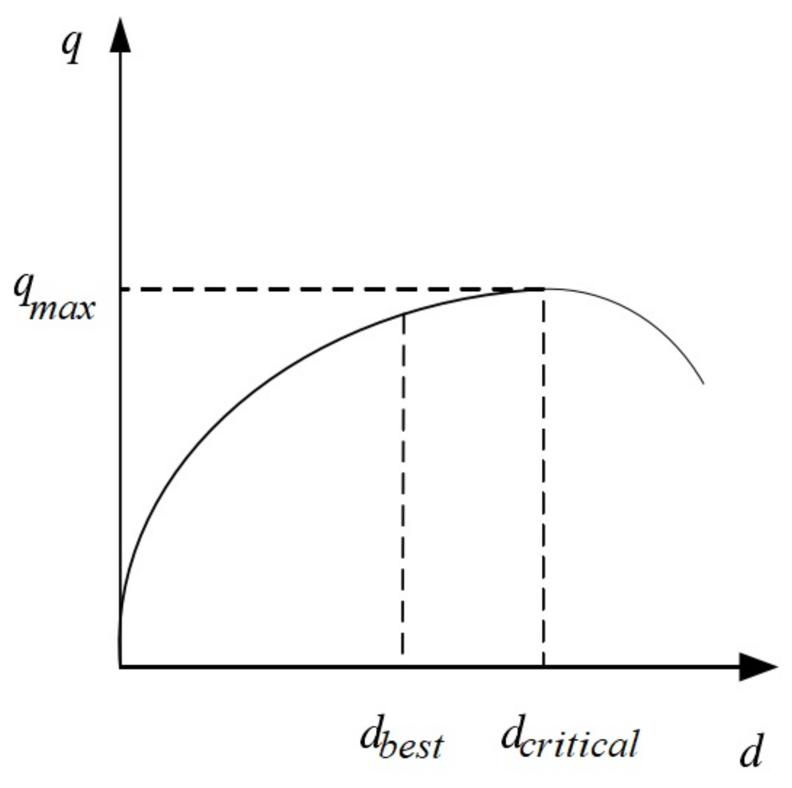
Quality Objective Function
- Quality-Duration Model
- 2.
- Quality–Period–Cost Model
Comprehensive Balanced Optimization Model
2.3. Model Solving
3. Results Analysis and Discussion
3.1. Example Verification
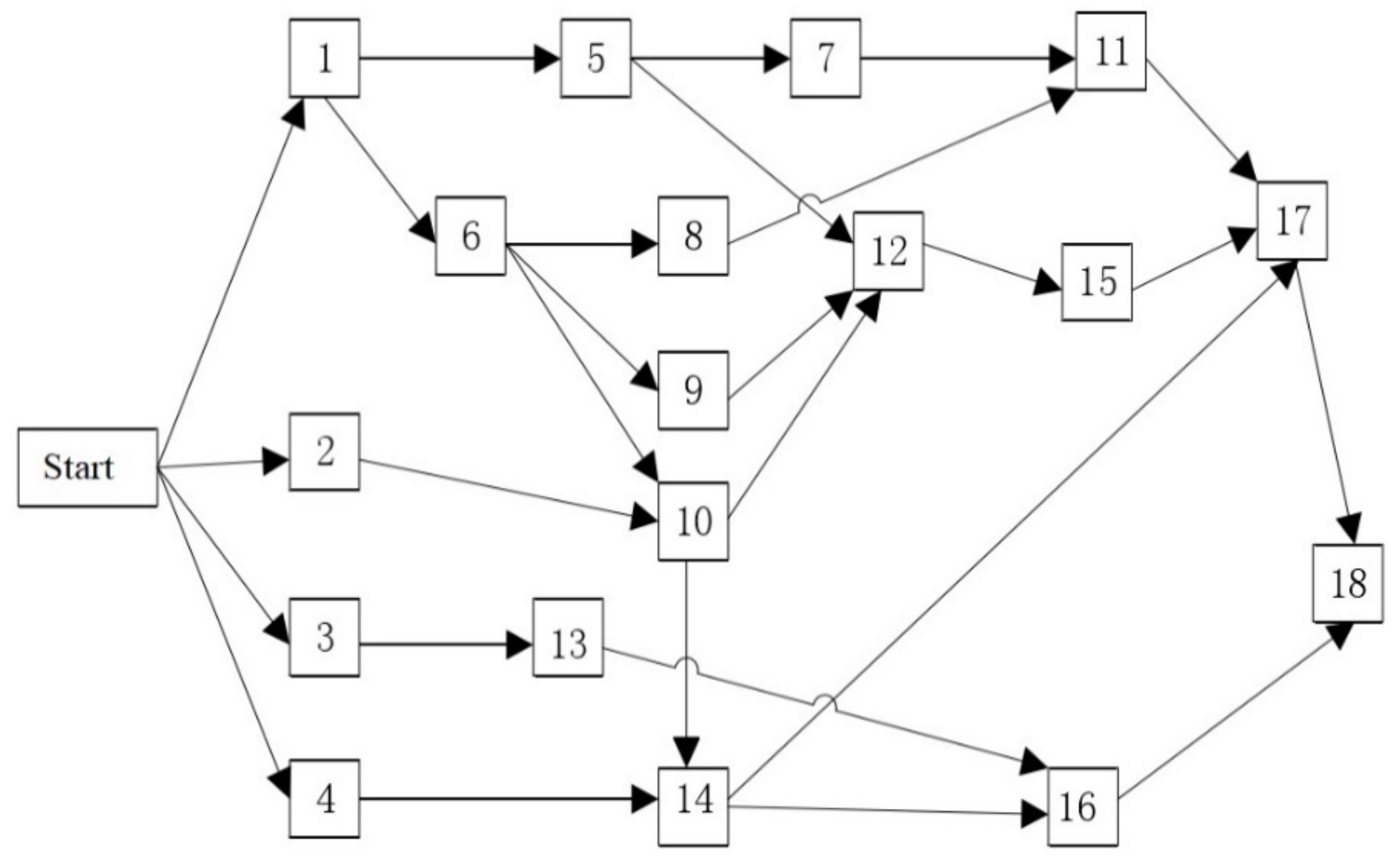
3.1.1. Introduction to Calculation Example
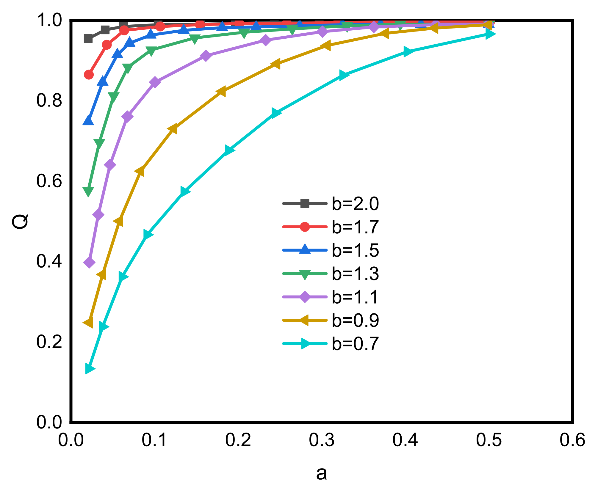
3.1.2. Parameter Selection
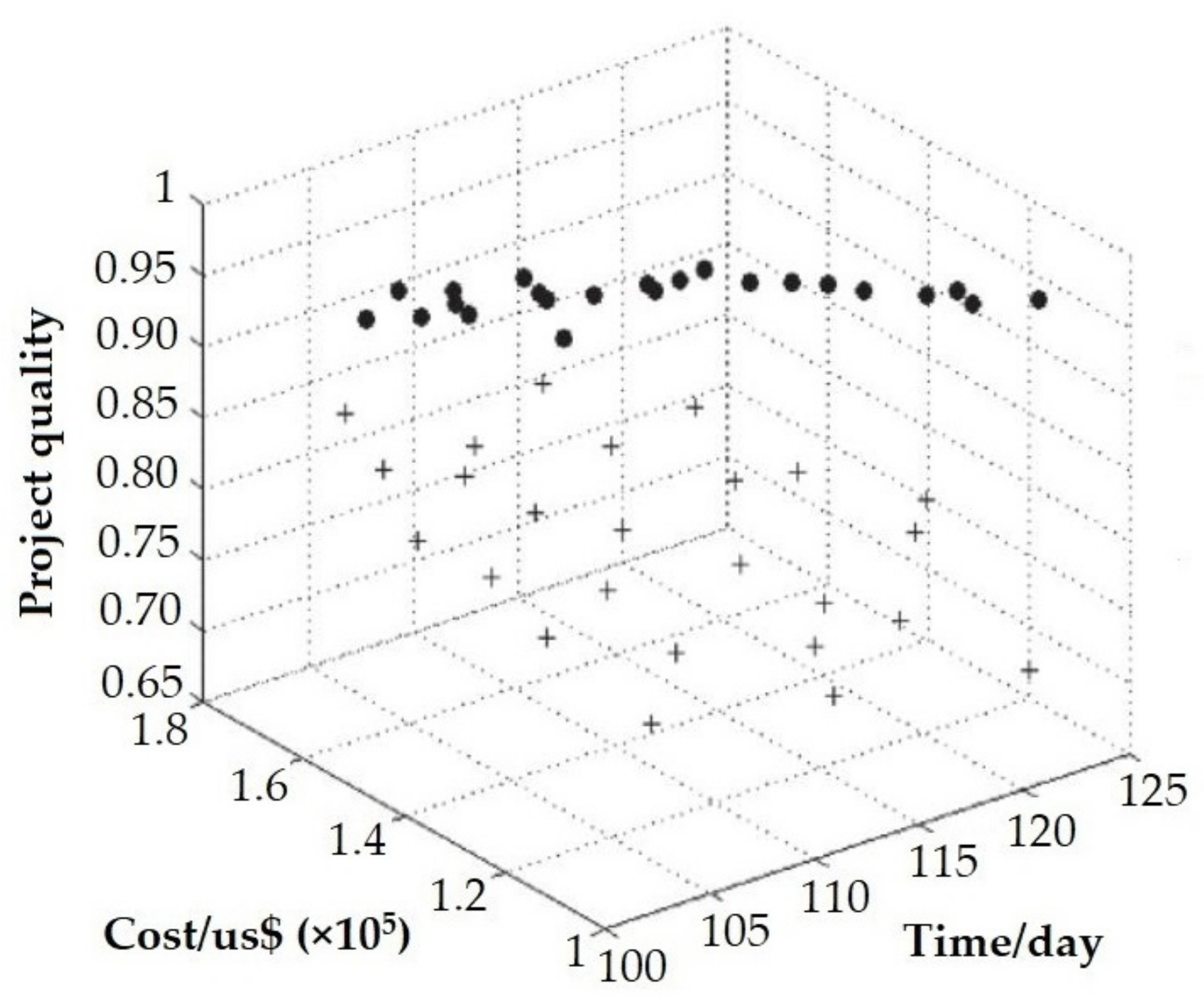
3.1.3. Engineering Applications
4. Conclusions
Author Contributions
Funding
Institutional Review Board Statement
Informed Consent Statement
Data Availability Statement
Conflicts of Interest
References
- Abdel-Basset, M.; Ali, M.; Atef, A. Uncertainty assessments of linear time-cost tradeoffs using neutrosophic set. Comput. Ind. Eng. 2020, 141, 106286. [Google Scholar] [CrossRef]
- Ammar, M.A. Optimization of Project Time-Cost Trade-Off Problem with Discounted Cash Flows. J. Constr. Eng. Manag. 2011, 137, 65–71. [Google Scholar] [CrossRef]
- Babu, A.; Suresh, N. Project management with time, cost, and quality considerations. Eur. J. Oper. Res. 1996, 88, 320–327. [Google Scholar] [CrossRef]
- Ballesteros-Pérez, P.; Elamrousy, K.M.; González-Cruz, M.C. Non-linear time-cost trade-off models of activity crashing: Application to construction scheduling and project compression with fast-tracking. Autom. Constr. 2018, 97, 229–240. [Google Scholar] [CrossRef] [Green Version]
- Duc-Hoc, T.; Min-Yuan, C.; Minh-Tu, C. Hybrid multiple objective artificial bee colony with differential evolution for the time–cost–quality trade-off problem. Knowl. Based Syst. 2015, 74, 176–186. [Google Scholar]
- Duc-Long, L.; Duc-Hoc, T.; Phong Thanh, N. Optimizing multi-mode time-cost-quality trade-off of construction project using opposition multiple objective difference evolution. Int. J. Constr. Manag. 2018, 21, 2327–2331. [Google Scholar]
- El-Rayes, K.; Kandil, A. Time-cost-quality trade-off analysis for highway construction. J. Constr. Eng. Manag. 2005, 131, 477–486. [Google Scholar] [CrossRef]
- Golpîra, H. Optimal integration of the facility location problem into the multi-project multi-supplier multi-resource Construction Supply Chain network design under the vendor managed inventory strategy. Expert Syst. Appl. 2020, 139, 112841. [Google Scholar] [CrossRef]
- Golpîra, H.; Sadeghi, H.; Khan, S. Time–Cost Trade-off Optimal Approaches. In Application of Mathematics and Optimization in Construction Project Management; Springer: Cham, Switzerland, 2021; pp. 119–140. [Google Scholar]
- Hadi, M.; Mahdi, B.; Ali, S. Three-Dimensional Time, Cost and Quality Tradeoff Optimization in Project Decision Making. Adv. Mater. Res. 2012, 433–440, 5746–5752. [Google Scholar]
- Hu, C. Optimization of Construction Schedule and Control Method in Hydroelectric Project; Tianjin University: Tianjin, China, 2015. (In Chinese) [Google Scholar]
- Khang, D.; Myint, Y. Time, cost and quality trade-off in project management: A case study. Int. J. Proj. Manag. 1999, 17, 249–256. [Google Scholar] [CrossRef]
- Mungle, S.; Benyoucef, L.; Son, Y. A fuzzy clustering-based genetic algorithm approach for time–cost–quality trade-off problems: A case study of highway construction project. Eng. Appl. Artif. Intell. 2013, 26, 1953–1966. [Google Scholar] [CrossRef]
- Rahimi, M.; Iranmanesh, H. Multi Objective Particle Swarm Optimization for a Discrete Time, Cost and Quality Trade-off Problem. World Appl. Sci. J. 2008, 4, 270–276. [Google Scholar]
- Tareghian, H.; Taheri, S. A solution procedure for the discrete time, cost and quality tradeoff problem using electromagnetic scatter search. Appl. Math. Comput. 2007, 190, 1136–1145. [Google Scholar] [CrossRef]
- Vedat, T.; MAzim, E. Time-Cost Trade-off Optimization of Construction Projects using Teaching Learning Based Optimization. KSCE J. Civ. Eng. 2019, 23, 10–20. [Google Scholar]
- Wang, B.; Gao, J.; Nie, X. Schedule optimization of water conservancy projectwith comprehensive consideration of cost-quality-completion risks. J. Hydroelectr. Eng. 2014, 33, 267–272. [Google Scholar]
- Xu, J.; Zhou, X. Fuzzy-Like Multiple Objective Decision Making; Springer: Berlin/Heidelberg, Germany, 2011. [Google Scholar]
- Zhang, H.; Xing, F. Fuzzy-multi-objective particle swarm optimization for time-cost-quality tradeoff in construction. Autom. Constr. 2010, 19, 1067–1075. [Google Scholar] [CrossRef]
- Zhang, L.; Du, J.; Zhang, S. Solution to the Time-Cost-Quality Trade-off Problems in Construction Projects based on Immune Genetic Particle Swarm Optimization. J. Manag. Eng. 2014, 30, 163–172. [Google Scholar] [CrossRef]


| Operation Quality Grade | Operation Quality Level | Operation Quality Evaluation |
|---|---|---|
| Level 1 | 0.9–1.0 | Excellent |
| Level 2 | 0.8–0.9 | Good |
| Level 3 | 0.7–0.8 | Qualified |
| Level 4 | 0.6–0.7 | Basic qualification |
| Level 5 | 0.6 or less | Failed |
| Operation Number | Scheme | ||||
|---|---|---|---|---|---|
| 1 | 1 | (13, 14, 15) | (13, 14, 15) | (2200, 2400, 2600) | 0.03 |
| 2 | (13, 15, 17) | (11, 13, 15) | (2000, 2150, 2300) | ||
| 3 | (14, 16, 18) | (9, 11, 13) | (1800, 1900, 2000) | ||
| 4 | (18, 21, 24) | (13, 16, 19) | (1400, 1500, 1600) | ||
| 5 | (22, 24, 26) | (11, 14, 17) | (1100, 1200, 1300) | ||
| 2 | 1 | (14, 15, 16) | (13, 14, 15) | (2000, 3000, 4000) | 0.05 |
| 2 | (17, 18, 19) | (14, 16, 18) | (2200, 2400, 2600) | ||
| 3 | (18, 20, 22) | (13, 16, 19) | (1700, 1800, 1900) | ||
| 4 | (21, 23, 25) | (15, 17, 19) | (1400, 1500, 1600) | ||
| 5 | (23, 25, 27) | (13, 15, 17) | (950, 1000, 1050) | ||
| 3 | 1 | (14, 15, 16) | (13, 15, 17) | (4000, 4500, 5000) | 0.08 |
| 2 | (20, 22, 24) | (17, 19, 21) | (3000, 4000, 5000) | ||
| 3 | (30, 33, 36) | (21, 23, 25) | (3000, 3200, 3400) | ||
| ⁝ | ⁝ | ⁝ | ⁝ | ⁝ | ⁝ |
| 18 | 1 | (8, 9, 10) | (7, 8, 9) | (2600, 3000, 3400) | 0.05 |
| 2 | (14, 15, 16) | (9, 11, 13) | (2100, 2400, 2700) | ||
| 3 | (16, 18, 20) | (7, 10, 13) | (2100, 2200, 2300) |
| Reference by Mungle et al. [12] Optimization Results | Duration/Day | Cost/US$ | Quality | Model 1—Optimized Results | Duration/Day | Cost/US$ | Quality | Model 2—Optimized Results | Duration/Day | Cost/US$ | Quality |
|---|---|---|---|---|---|---|---|---|---|---|---|
| 1 | 104 | 168,480 | 0.85667 | 1 | 104 | 164,168 | 0.9319 | 1 | 104 | 164,015 | 0.9245 |
| 2 | 104 | 160,860 | 0.83167 | 2 | 104 | 157,410 | 0.9421 | 2 | 105 | 158,328 | 0.9028 |
| 3 | 104 | 153,968 | 0.79600 | 3 | 105 | 162,180 | 0.9502 | 3 | 105 | 152,275 | 0.8902 |
| 4 | 105 | 143,345 | 0.78634 | 4 | 106 | 152,105 | 0.9487 | 4 | 106 | 160,478 | 0.9103 |
| 5 | 106 | 153,120 | 0.83233 | 5 | 106 | 154,830 | 0.9505 | 5 | 107 | 155,320 | 0.8911 |
| 6 | 106 | 136,858 | 0.75267 | 6 | 106 | 155,230 | 0.9592 | 6 | 108 | 146,450 | 0.8709 |
| 7 | 107 | 155,130 | 0.84534 | 7 | 108 | 141,518 | 0.9438 | 7 | 109 | 141,870 | 0.8585 |
| 8 | 108 | 147,460 | 0.80800 | 8 | 108 | 144,990 | 0.9644 | 8 | 110 | 138,520 | 0.8484 |
| 9 | 108 | 124,110 | 0.70734 | 9 | 108 | 146,760 | 0.9652 | 9 | 110 | 134,335 | 0.8436 |
| 10 | 109 | 136,975 | 0.77100 | 10 | 108 | 149,528 | 0.9693 | 10 | 111 | 152,820 | 0.9214 |
| 11 | 110 | 127,688 | 0.74067 | 11 | 109 | 139,760 | 0.9716 | 11 | 112 | 145,227 | 0.9005 |
| 12 | 111 | 158,415 | 0.86234 | 12 | 111 | 137,520 | 0.9741 | 12 | 113 | 131,310 | 0.8663 |
| 13 | 111 | 142,308 | 0.79267 | 13 | 111 | 136,075 | 0.9729 | 13 | 114 | 128,900 | 0.8480 |
| 14 | 112 | 149,030 | 0.83300 | 14 | 112 | 135,210 | 0.9778 | 14 | 116 | 122,175 | 0.8325 |
| 15 | 114 | 131,568 | 0.77434 | 15 | 113 | 134,360 | 0.9809 | 15 | 118 | 135,508 | 0.8767 |
| 16 | 114 | 116,618 | 0.74734 | 16 | 114 | 129,430 | 0.9772 | 16 | 119 | 114,070 | 0.8228 |
| 17 | 114 | 113,118 | 0.71967 | 17 | 115 | 125,508 | 0.9803 | 17 | 120 | 125,805 | 0.8404 |
| 18 | 116 | 148,870 | 0.84134 | 18 | 116 | 122,310 | 0.9797 | 18 | 121 | 117,960 | 0.8117 |
| 19 | 116 | 140,870 | 0.80500 | 19 | 117 | 119,430 | 0.9771 | 19 | 122 | 133,520 | 0.8520 |
| 20 | 118 | 123,050 | 0.75500 | 20 | 119 | 115,250 | 0.9726 | 20 | 122 | 120,933 | 0.8383 |
| 21 | 119 | 116,340 | 0.74567 | 21 | 120 | 113,350 | 0.9738 | 21 | 123 | 109,268 | 0.8003 |
| 22 | 121 | 140,815 | 0.79600 | 22 | 120 | 110,270 | 0.9712 | ||||
| 23 | 123 | 126,060 | 0.77334 | 23 | 123 | 109,550 | 0.9603 | ||||
| 24 | 123 | 132,000 | 0.77534 | ||||||||
| 25 | 123 | 111,355 | 0.69600 |
| Operation Number | Scheme | |||
|---|---|---|---|---|
| 1 | 1 | (1, 2, 3) | (7,575,757; 8,333,333; 9,090,909) | (0.90, 0.92, 0.94) |
| 2 | (2, 3, 4) | (6,666,666; 7,272,727; 7,878,787) | (0.88, 0.89, 0.90) | |
| 2 | 1 | (3, 4, 5) | (9,242,424; 10,151,515; 11,060,606) | (0.83, 0.86, 0.89) |
| 2 | (4, 5, 6) | (8,636,363; 9,393,939; 10,151,515) | (0.74, 0.76, 0.78) | |
| 3 | 1 | (2, 3, 4) | (8,484,848; 8,939,393; 9,393,939) | (0.70, 0.72, 0.74) |
| 2 | (3, 4, 5) | (7,878,787; 8,333,333; 8,787,878) | (0.81, 0.82, 0.83) | |
| 3 | (4, 5, 6) | (7,272,727; 7,727,272; 8,181,818) | (0.78, 0.80, 0.82) | |
| 4 | 1 | (2, 3, 4) | (3,484,848; 3,787,878; 4,090,909) | (0.85, 0.86, 0.87) |
| 2 | (3, 4, 5) | (2,878,787; 3,181,818; 3,484,848) | (0.80, 0.83, 0.86) | |
| 5 | 1 | (4, 5, 6) | (6,363,636; 6,818,181; 7,272,727) | (0.92, 0.94, 0.96) |
| 2 | (5, 6, 7) | (5,606,060; 6,060,606; 6,515,151) | (0.87, 0.89, 0.91) | |
| 6 | 1 | (1, 2, 3) | (5,454,545; 5,757,575; 6,060,606) | (0.75, 0.77, 0.79) |
| 2 | (2, 3, 4) | (4,924,242; 5,303,030; 5,681,818) | (0.96, 0.97, 0.98) | |
| 3 | (3, 4, 5) | (4,621,212; 4,848,484; 5,075,757) | (0.91, 0.92, 0.93) | |
| 7 | 1 | (7, 8, 9) | (8,181,818; 8,484,848; 8,787,878) | (0.78, 0.79, 0.80) |
| 2 | (9, 10, 11) | (7,500,000; 7,727,272; 7,954,545) | (0.76, 0.77, 0.78) | |
| 3 | (10, 12, 14) | (6,818,181; 6,969,696; 7,121,212) | (0.70, 0.73, 0.76) | |
| 8 | 1 | (1, 2, 3) | (5,303,030; 5,454,545; 5,606,060) | (0.86, 0.87, 0.88) |
| 2 | (2, 3, 4) | (4,848,484; 5,000,000; 5,151,515) | (0.84, 0.85, 0.86) | |
| 3 | (3, 4, 5) | (3,636,363; 4,545,454; 5,454,545) | (0.80, 0.82, 0.84) | |
| 9 | 1 | (1, 2, 3) | (2,348,484; 2,878,787; 3,409,090) | (0.97, 0.98, 0.99) |
| 2 | (2, 3, 4) | (1,742,424; 2,121,212; 2,500,000) | (0.94, 0.96, 0.98) | |
| 10 | 1 | (1, 2, 3) | (3,106,060; 3,787,878; 4,469,696) | (0.88, 0.90, 0.92) |
| 2 | (2, 3, 4) | (2,954,545; 3,333,333; 3,863,636) | (0.86, 0.88, 0.90) | |
| 11 | 1 | (1, 2, 3) | (757,575; 909,090; 1,060,606) | (0.91, 0.94, 0.97) |
| 2 | (2, 3, 4) | (454,545; 606,060; 757,575) | (0.79, 0.83, 0.87) |
| Solution Number | Duration/Month | Cost/US$ | Quality |
|---|---|---|---|
| 1 | 43 | 82,575,757 | 0.8032 |
| 2 | 41 | 83,787,878 | 0.8145 |
| 3 | 40 | 84,545,454 | 0.8280 |
| 4 | 38 | 85,606,060 | 0.8316 |
| 5 | 37 | 86,666,666 | 0.8457 |
| 6 | 36 | 87,727,272 | 0.8621 |
| 7 | 34 | 88,484,848 | 0.8658 |
| 8 | 32 | 89,696,969 | 0.8796 |
Publisher’s Note: MDPI stays neutral with regard to jurisdictional claims in published maps and institutional affiliations. |
© 2022 by the authors. Licensee MDPI, Basel, Switzerland. This article is an open access article distributed under the terms and conditions of the Creative Commons Attribution (CC BY) license (https://creativecommons.org/licenses/by/4.0/).
Share and Cite
Mendomo Meye, S.; Li, G.; Shen, Z.; Zhang, J. Fuzzy Multi-Mode Time–Cost–Quality Trade-Off Optimization in Construction Management of Hydraulic Structure Projects. Appl. Sci. 2022, 12, 6270. https://doi.org/10.3390/app12126270
Mendomo Meye S, Li G, Shen Z, Zhang J. Fuzzy Multi-Mode Time–Cost–Quality Trade-Off Optimization in Construction Management of Hydraulic Structure Projects. Applied Sciences. 2022; 12(12):6270. https://doi.org/10.3390/app12126270
Chicago/Turabian StyleMendomo Meye, Serges, Guowei Li, Zhenzhong Shen, and Jingbin Zhang. 2022. "Fuzzy Multi-Mode Time–Cost–Quality Trade-Off Optimization in Construction Management of Hydraulic Structure Projects" Applied Sciences 12, no. 12: 6270. https://doi.org/10.3390/app12126270