A New Robust Method to Investigate Dynamic Instability of FTV for the Double Tripod Industrial Driveshafts in the Principal Parametric Resonance Region

Featured Application

Time–history analysis (THA), the Lyapunov Exponents Approach (LEA), and the Poincaré Map (PM) are enhanced to investigate the dynamic instability of forced torsional vibrations (FTV) for a double tripod industrial driveshaft (DTID) in transition through the principal parametric resonance region (PPRR). Based on a modified designed model of FTV for an automotive driveshaft (AD), a robust method comprising THA, LEA, and PM (THA–LEA–PM) was created that certifies the existence of deterministic chaos or an ergodic process for the dynamic behavior of DTID’s FTV in transition through PPRR. These methods represent a design tool for the DTID’s FTV control of the homokinetic driveline transmission in the industry.

Abstract

The present work aims to design a robust method to detect and certify the deterministic chaos or ergodic process for the forced torsional vibrations (FTV) of a double tripod industrial driveshaft (DTID) in transition through the principal parametric resonance region (PPRR) which is considered by the researchers in the field as one of the most important resonance regions for the systems having parametric excitations. The DTID’s model for FTV considers the following effects: nonuniformities of inertial characteristics of the DTID’s elements, the harmonic torque excitation induced by the asynchronous electrical motor used for a heavy-duty grain mill, and the harmonic reaction torque generated by different granulation of the substance needed to be milled. Based on these aspects, a model of the FTV for the DTID was designed which was a modified, physically consistent model already used by the authors to investigate the FTV of automotive driveshafts (homokinetic transmission). For the DTID elements, the dynamic instability for nonstationary FTV in the PPRR using time–history analysis (THA) was analyzed—THA represents the phase portraits. Time–history analysis is a detection method for possible chaotic dynamic behavior for the nonstationary FTV (NFTV) in transition through PPRR. If this dynamic behavior was seen, a new robust method LEA–PM was created to certify and confirm the deterministic chaos for the NFTV of DTID. The new method, LEA–PM, is composed of the Lyapunov exponent’s approach (LEA) coupled with the Poincaré Map (PM) applied to the global system of differential equations that describe the FTV of DTID in the PPRR. This new robust method, which embeds LEA and PM, LEA–PM, establishes if the mechanical system has a deterministic chaotic dynamic behavior (strange attractor) or an ergodic dynamic process in this resonant region. LEA represents a new method that includes not only the maximal Lyapunov exponent method (MLEM) but also new mathematical criteria that is “the sum of all Lyapunov exponents has to be negative” which, coupled with MLEM, indicates the presence of deterministic chaos (strange attractors). THA–LEA–PM had been used for the NFTV of DTID computing the phase portraits, the Lyapunov exponents, and representing the Poincaré Maps of the NFTV for the DTID’s elements in transition through PPRR, founding deterministic chaos or ergodic dynamic behavior. Based on the obtained results, numerical simulations revealed the pitting manifestations of the DTID’s elements, typical for the geared systems transmission, mentioned recently in experimental data research for the homokinetic transmissions. Using the new robust method, THA–LEA–PM (time–history analysis coupled with LEA–PM) can be used in future research for chaotic dynamic analysis of DTID’s NFTV transition through superharmonic resonances, subharmonic resonances, combination resonances, and internal resonances. Time–history analysis as a detection method for chaos and LEA–PM as a certifying method for deterministic chaos can be integrated as a design tool for DTID’s FTV control of the homokinetic transmission.

1. Introduction

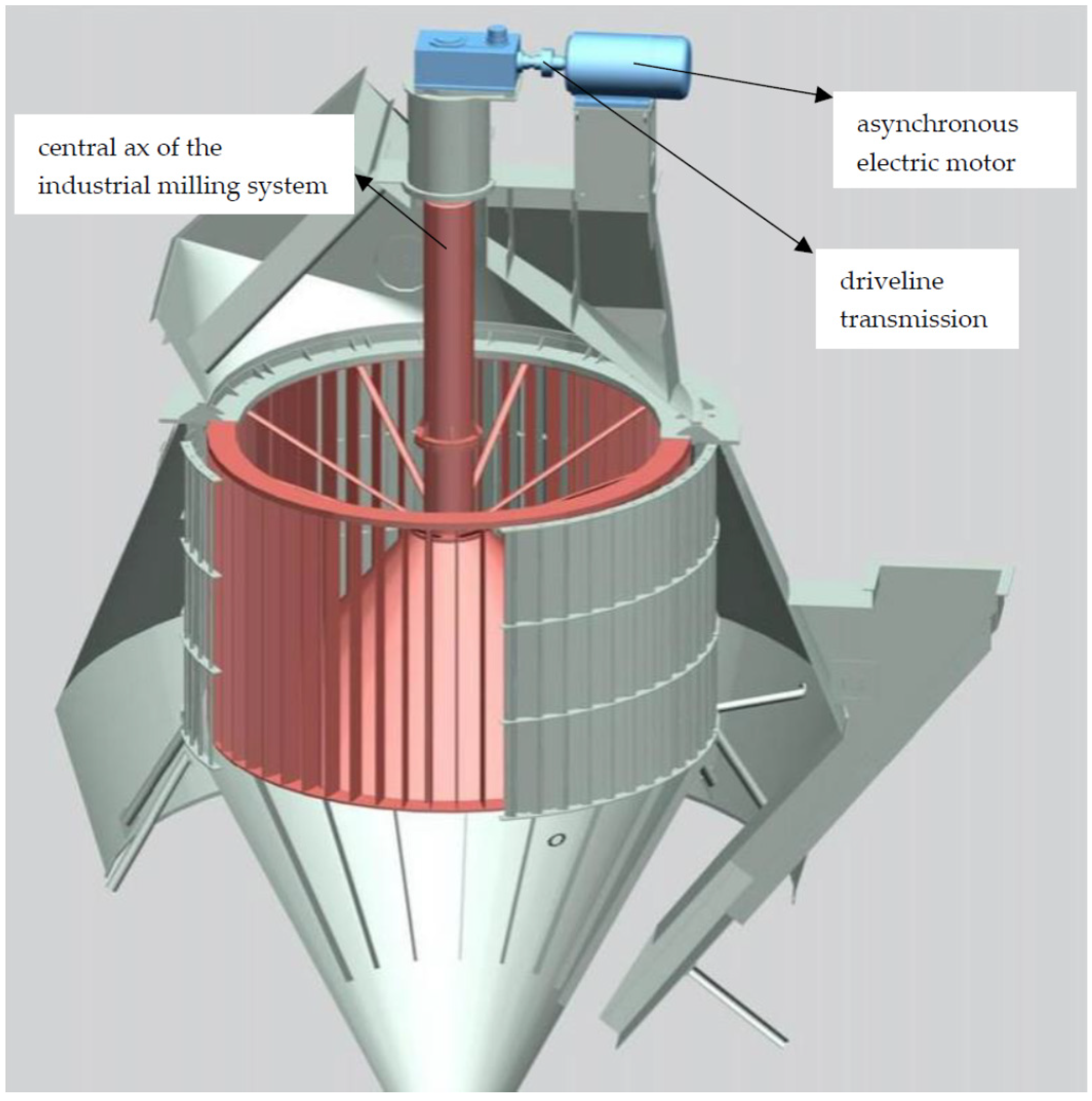
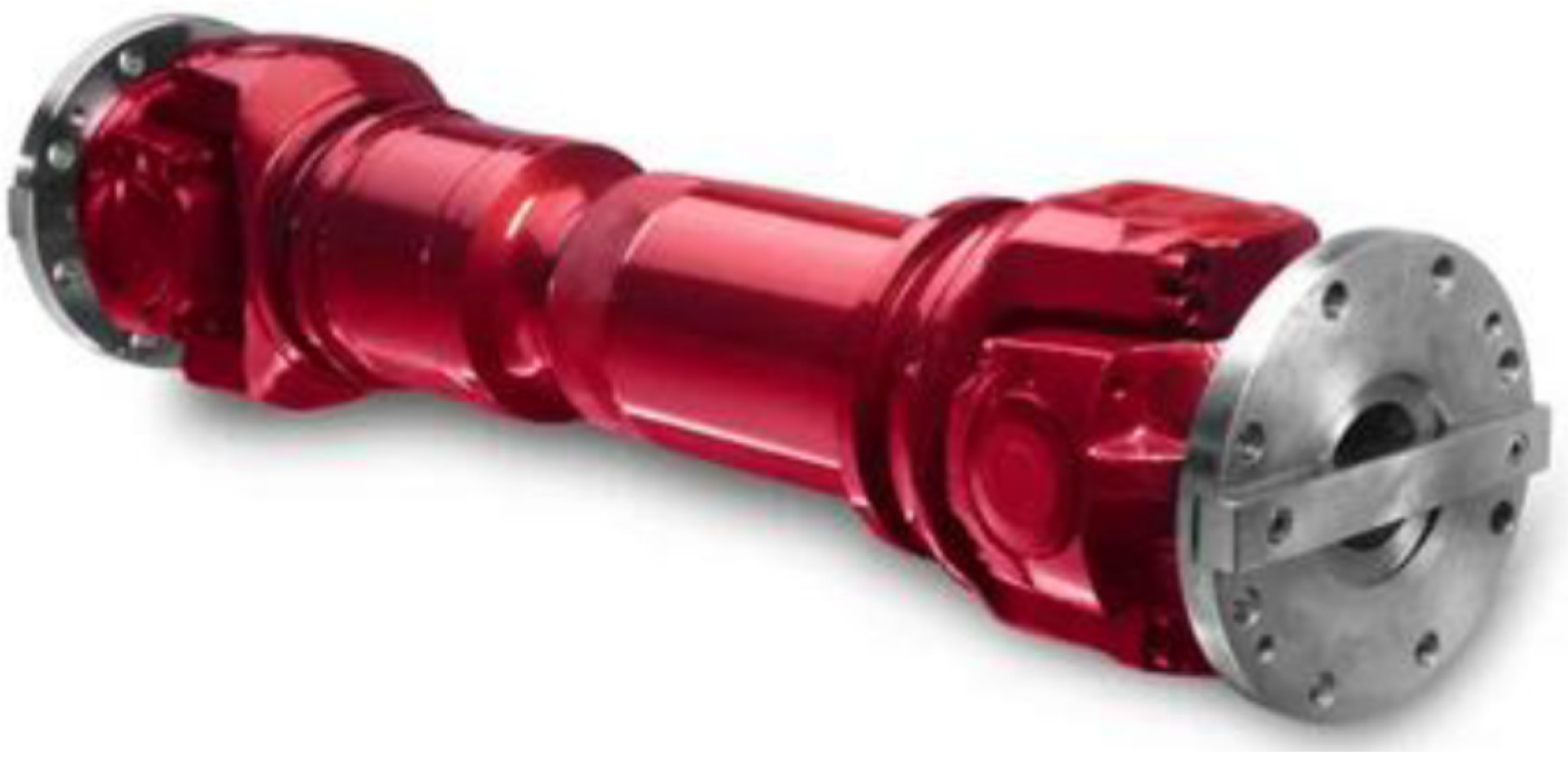
The double tripod industrial driveshafts (DTID) are used in the cement industry plant, food industry, and agriculture industry to link the power supplier with the industrial mill. In most cases, the power supplier is the asynchronous electric motors, and the link to a moderate heavy-duty mill is DTID, the industrial system presented in Figure 1. Generally, in heavy-duty use, a drivetrain line from the electric motor to the mill is covered by a double cardan driveshaft, see Figure 2, but this type of driveshaft, having two Hooke’s joints, induces a nonuniformity that must be avoided [1] (pp. 5–9).

For a moderate heavy-duty industrial milling system, to avoid the non-uniformity of Hooke’s joints, a double tripod industrial driveshaft (DTID) is used in the driveline transmission because this type of driveshaft has two constant velocity joints (CVJ) [1] (pp. 52–79). The DTIDs are, in fact, quasi-homokinetic driveshafts, as proven by Dudita et al. [1] (p. 78), in [2], and mentioned in [3]. This is the type of DTID that the present work deals with, and the first effect considered is the kinematic nonuniformity already studied in detail by the papers [2,3]. Qiu et al. developed [4] a double roller tripod joint to obtain a better constant velocity. The excitation torque load, an input of the asynchronous electric motor, can be considered harmonic type, as mentioned by Miljkovic in the paper [5]. The present work investigates nonstationary forced torsional vibrations (NFTV) of DTID using designed methods that certify the possible chaotic deterministic or ergodic dynamic behavior. In [6], Rossi et al. developed a torsional model with two degrees of freedom (2 DOF) to investigate the damping of torsional vibrations in variable speed drive, particularly the torsional mode excitations. Xu et al. studied [7] the amplitude-frequency characteristics for torsional vibration in an automotive powertrain using a model with 29 DOF. In his doctoral thesis [8] (pp. 6–100), Yao investigated the modeling of nonlinear driveshaft systems with double U-joints, observing the passage effect and the Sommerfeld effect for both 2 DOF and 3 DOF models. Based on findings in the literature [6,7,8], it is evident, in opposition to the models in [9], that the modified physically consistent model (MPCM) for FTV of DTID is a better approach to industrial realities. The next paragraph will discuss the MPCM for FTV of DTID that considers the following aspects: double tripod of the joints for ID, geometric and kinematic nonuniformity of CVJs, and harmonic excitation of torsional torque load due to the use of an asynchronous electric motor for the moderate heavy-duty industrial milling system as well as the reactive harmonic torque induced by the mill. In their paper, Mazzei and Scott remarked for the first time using numerical data [10] that the most critical resonance for a driveshaft with a universal joint is the principal parametric resonance. SoltanRezzaee et al. in the article [11], investigated the parametric instability of driveshafts with U-joints using the monodromy matrix method. Another study [12] investigated the dynamic instability of a double cardan joint using the FEM (finite element method) coupled with the monodromy matrix method. As suggested in the literature [10,11,12], the most crucial resonant case of a driveshaft is the principal parametric resonance; therefore, the present work is dedicated to investigating the nonstationary dynamic instability of FTV for DTID in the principal parametric resonance region (PPRR). Loginovskikh et al. [13] investigated the values of tangential stress for a pumping unit shaft in the resonant case, confirming the need for avoiding such a torsional resonance region. The paper [14] studied the designing needs of models for torsional vibrations of shafts of mechanical systems to control the dynamic behavior in torsion, by vibration dampers and equivalent stiffness of double-mass oscillating systems. Zhai et al. [15] investigated the vibration characteristics of the shaft systems for dredging pumps using the FEM to determine the upper and the lower limits for critical speeds of torsional vibration. It was observed that the rated speed of the dredging pump was far less than the predicted critical speed. Therefore, FEM offers only some reference value on the stability analysis of the shaft system. Experimental investigations and finite element analysis were carried out in the literature [16] to determine the natural frequencies and the mode shapes for steel and CFRP (carbon fiber reinforced plastic) driveshafts. This interest in CFRP is due to the advantages afforded to the industry when using CFRP instead of steel. Mazzei and Scott demonstrated through [17] that a method of avoiding parametric resonances of the universal joint driveline is accelerating through these regions. As identified in the literature [13,14,15,16,17], it is necessary to investigate the PPRR locally and globally in close detail. Steinwede, in his Ph.D. thesis [18] (pp. 88–94), experimentally found the pitting and the microcracks on the tripod of the driveshaft. He explained that the driveshaft joints have similar dynamic behavior as the geared system transmission [18] (p. 117). Additionally, he stated that the bending and torsion vibrations manifest a “strange beating behavior” [18] (pp. 138–139) that is generated by the engine excitation, geometric and mass nonuniformities, and kinematic nonuniformity of joints. In the literature, the investigation of the chaotic behavior of the geared system transmission was performed in [19] (pp. 102–103, 127–131), and it was found that geared systems may have a deterministic chaos vibration that conducts in time to phenomena as pitting and microcracks. These aspects mentioned before must be investigated. One of the present paper’s goals is to investigate possible chaotic dynamic behavior for the NFTV in transition through PPRR. Kecik and Warminski [20] investigated the chaotic motion of an auto-parametric system by simulations using the maximal Lyapunov exponent method (MLEM) and laboratory experiments. In [21], Chang studied the control over chaotic behavior of an active magnetic bearing system by MLEM, Poincaré Maps, and phase portraits. Bavi et al. investigated the simultaneous resonance and stability analysis of unbalanced asymmetric thin-walled composite shafts in [22] using the multiple-scale approach (MSA) and the phase portrait graphs. As identified in [20,21,22], the methods of investigating the chaotic dynamic behavior are the MLEM (quantitative method) and the Poincaré Maps method (qualitative method), and for the computation of dynamic instability frontiers regions the perturbation approach MSA is used. The present paper will use time–history analysis to detect the dynamic chaotic behavior using the phase portrait graphs of the NFTV for DTID. The chaos will be investigated using a robust designed method given by the modified Lyapunov exponent’s method (MLEM) coupled with Poincaré Maps (PM), that is, Lyapunov Exponents Approach-Poincaré Map (LEA–PM), of the NFTV for DTID in transition through PPRR. These are the novel aspects of the new method: detection of chaos by analysis of time–history and investigation of chaos by employing LEA–PM. Why is this new and “mathematical affordable” method used by the designers of DTID? As mentioned before, most researchers, such as in [21], use MLEM directly without detecting chaos before. The new robust method detects possible chaotic behavior. Additionally, the MLEM is not sufficient for deterministic chaotic behavior, as mentioned in [23], and for this reason, MLEM was modified in a more complex new method, LEA. All the research on chaos manifestations needed a second confirmation for the deterministic chaos (the manifestation of strange attractors) due to the complexity of the dynamic phenomena when chaos occurs. Accordingly, the new method involves using a qualitative second method, the PM. Therefore, the new method LEA–PM becomes a robust method of investigating chaos. The new method is an equivalent method to investigate the chaos of dynamical systems in the simplest Riemannian spaces (spaces with Euclidian metrics). In contrast, the KCC method [24] is the newest method of investigating chaos for the higher-order dynamical systems in Finsler spaces. The KCC method is not a “mathematical affordable” method, such as LEA–PM, for the designers because it involves the management of spaces with two different metrics as Finsler spaces (the problem of curvature properties of homogeneous Finsler spaces with $\left(\mathsf{\alpha },\mathsf{\beta }\right)$-metrics is one of the central problems in Riemann–Finsler geometry) and the Jacobi stability analysis using KCC. In conclusion, the novelty of this work consists in introducing a new robust method with two-step detection and certification of the deterministic chaos for NFTV of DTID based on an MPCM of FTV that considers the following phenomena: nonuniformity of geometric and mass characteristics of the DTID, the kinematic nonuniformity of the DTID’s homokinetic joints, and the multiple harmonic excitations induced by the asynchronous electric motor and the milling system. The present research challenges are the investigation of NFTV of DTID using time–history analysis, phase portraits for possible chaos detection, and LEA–PM for deterministic chaos or nonstationary dynamic ergodic behavior of DTID in PPRR. This goal of the present work is the theoretical investigation of the pitting manifestation for the homokinetic transmissions, particularly the DTID mentioned by Steinwede [18] (pp. 138–139) for the automotive driveshaft and explained by the similarity with chaotic manifestations of the geared systems transmission [19] (pp. 102–103, 127–131) for which pitting and microcracks are common manifestations. Therefore, the aim of the work is the design of a new robust method to detect and confirm, without any doubt, the existence or not of deterministic chaos for the nonstationary FTV of a double tripod industrial driveshaft in the principal parametric resonance region. The novelty of this new method consists of using time–history analysis (THA represents the analysis of the phase portraits) as a detection method of possible chaos manifestation coupled with a new method, LEA–PM, to certify the existence of deterministic chaos. The LEA–PM has certain advantages because it is based not only on the MLEM (maximal Lyapunov exponent method) and using on the Poincaré Maps Method to reconfirm the deterministic chaos. The novelty of the present work is the design of the new robust method THA–LEA–PM that detects and certifies the deterministic chaos for NFTV of DTID’s elements in transition through PPRR. Additionally, the new LEA (Lyapunov exponent approach) combines the classic MLEM with a new criterion (the sum of Lyapunov exponents must be negative), as mentioned in [23]. In the meantime, THA–LEA–PM is much simpler to use, from a mathematical point of view, than KCC, as mentioned above.

2. The Modified Physically Consistent Model of FTV for Double Tripod Industrial Driveshaft

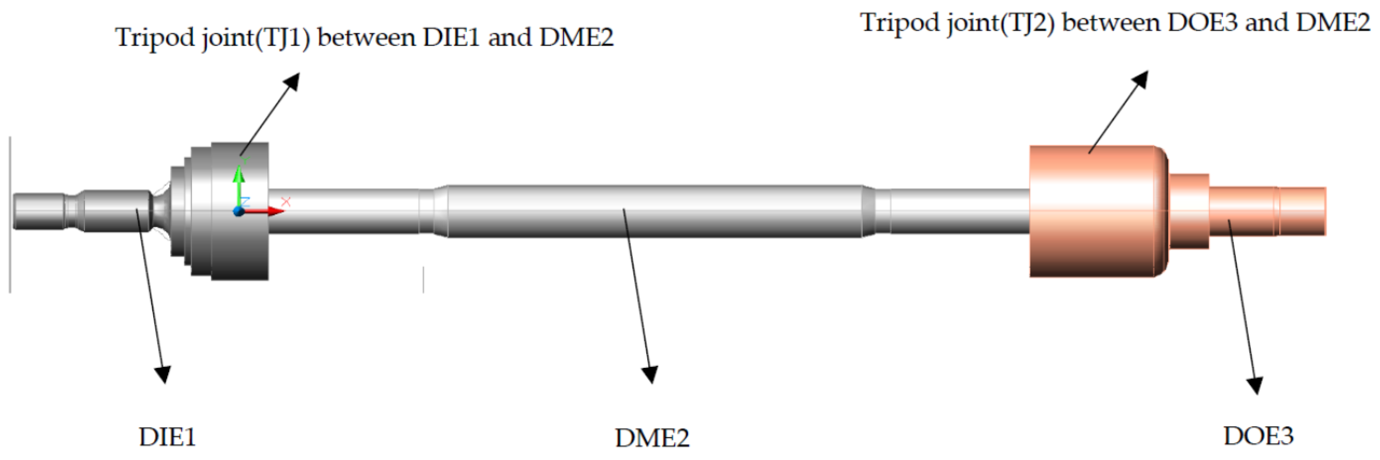
A DTID is a driveline transmission from an electric motor to a milling system composed of three elements: driven input element (DIE1), driving midshaft part (DME2), and driving output element (DOE3), as presented in Figure 3. The tripod joint is shown in detail in Figure 4. The DTID is rigidly fixed in the gearbox of the asynchronous electric motor through a spline assembly of the DIE1, see Figure 4, and is linked to the milling system through a similar spline assembly (see Figure 4).

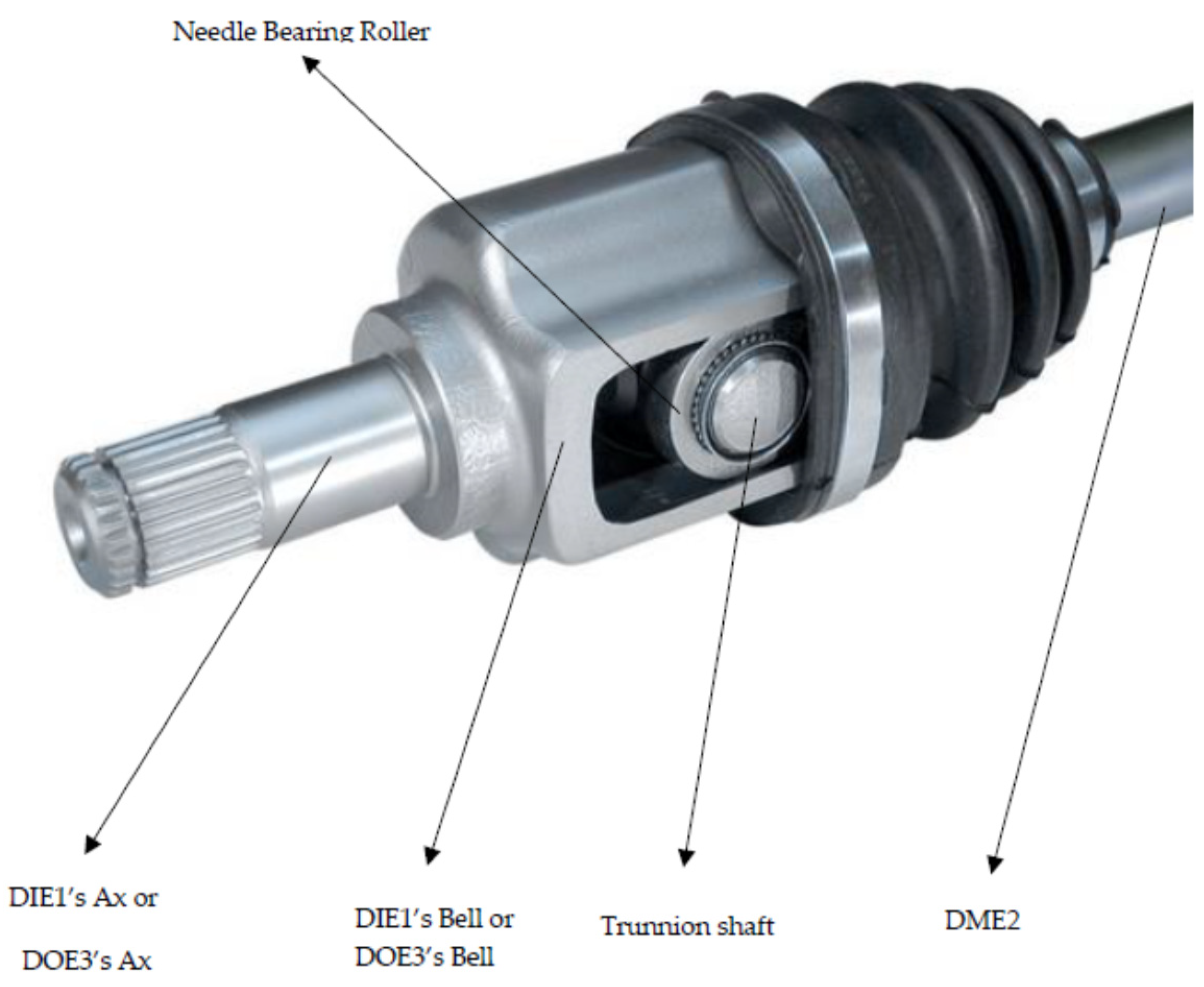
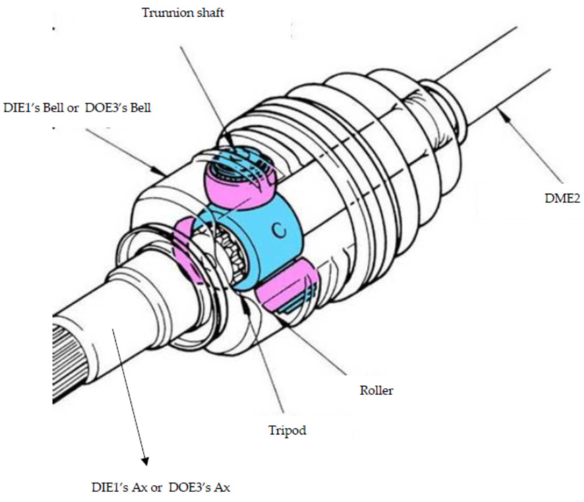
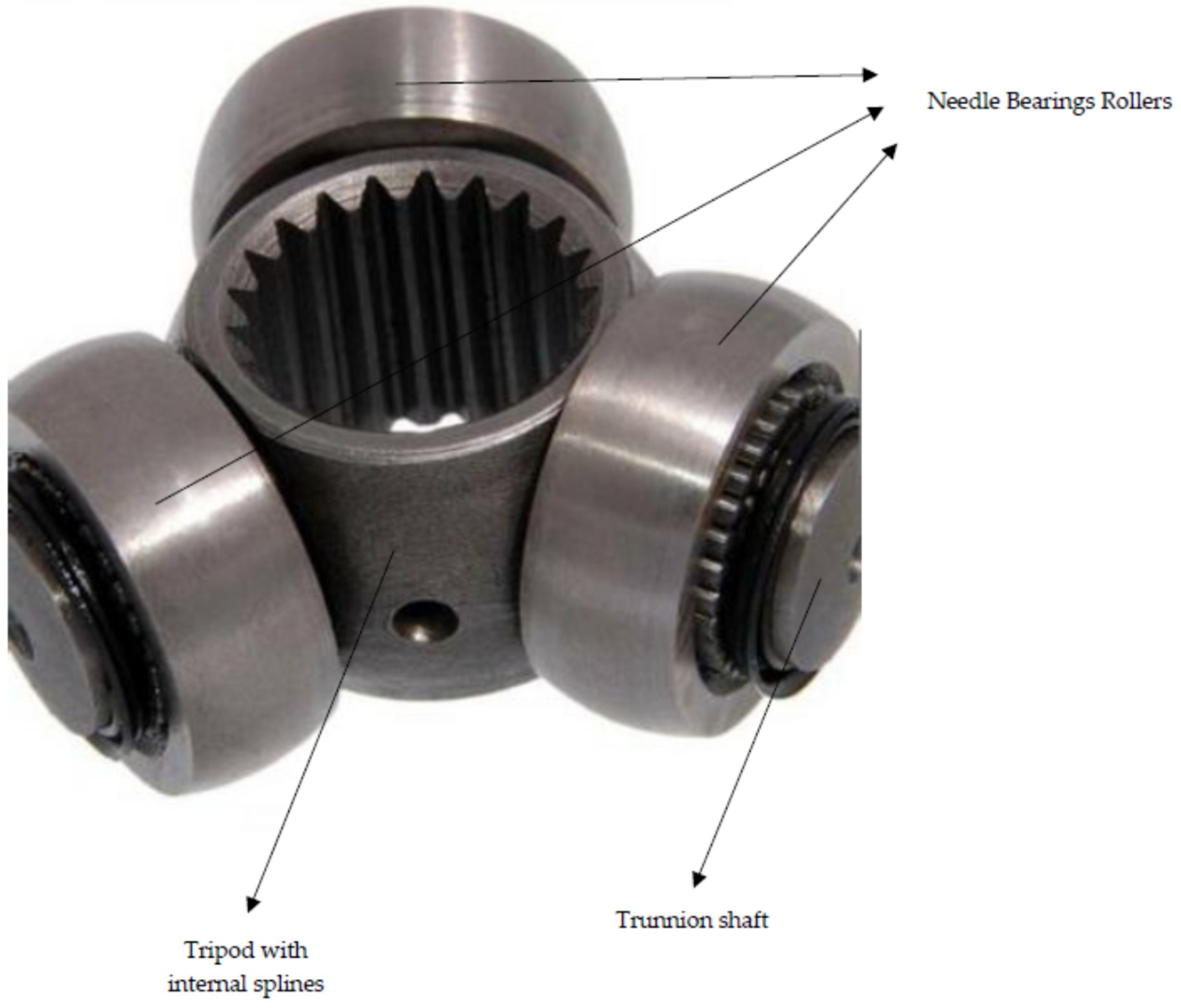
As shown in Figure 4, both tripods are fixed through splines on the DME2 at both ends of the midshaft and can plunge inside the bells of DIE1 and DOE3. Figure 5 is a tripod with three trunnion shafts with a distance of 120° between them, fixed on a tubular element with internal splines, and a needle-bearing roller is fixed on each trunnion shaft.

Figure 6 shows a picture of a DTID’s DIE1 or DOE3 with a section on the bell to show the trunnion shaft and a needle-bearing roller.

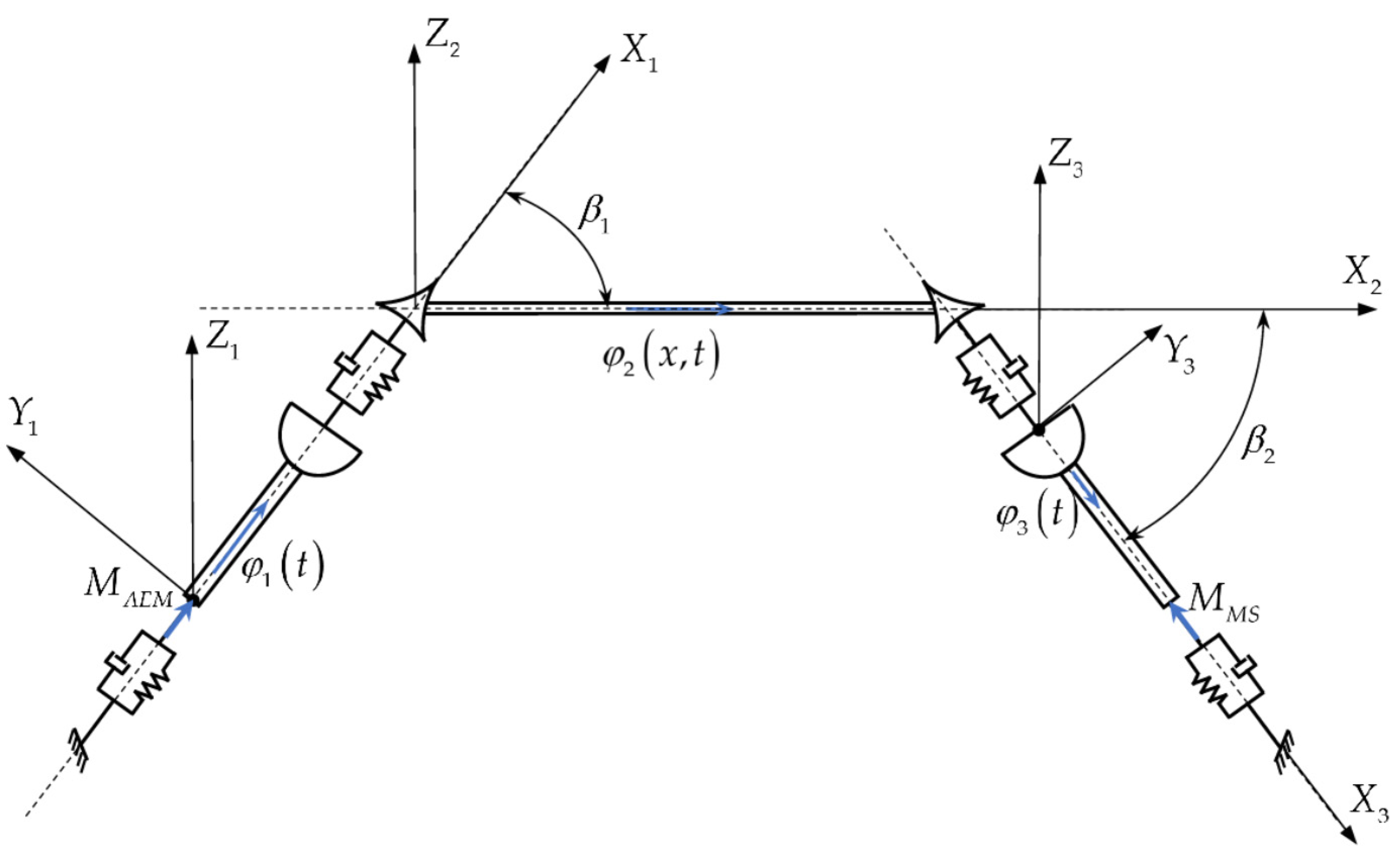
As seen in Figure 3, Figure 4, Figure 5 and Figure 6, the DTID is a multi-body system. Each element is attached to a cartesian system, as shown in Figure 7, and it is considered that the parts DIE1 and DOE3 have rigid twisting body motions along the longitudinal axes. In contrast, the element DME2 has an elastic continuous twisting motion along the longitudinal axis ${\mathrm{X}}_2$. The axes ${\mathrm{Z}}_1,{\mathrm{Z}}_2,{\mathrm{Z}}_3$ are parallel, therefore the planes $\left({\mathrm{X}}_1,{\mathrm{Y}}_1\right),$ $\left({\mathrm{X}}_2,{\mathrm{Y}}_2\right)$, and $\left({\mathrm{X}}_3,{\mathrm{Y}}_3\right)$ are coplanar. The angles ${\mathsf{\beta }}_1,{\mathsf{\beta }}_2$ are due to the misalignments between the output axis of the electric motor’s gearbox and the ax of the milling system being in the range of 0–9°.

The inertial characteristics for each element of the DTID are reduced to the longitudinal axis ${\mathrm{X}}_2$ (see Figure 7). All the axial geometric and the axial mass moments of inertia (AGMI and AMMI) for DIE1, DME2, and DOE3 are presented in Appendix A. The significance of the AGMI and AMMI expressed in Appendix A is: ${\mathrm{J}}_{{\mathrm{X}}_2\mathrm{D}\mathrm{I}\mathrm{E}1}$, ${\mathrm{I}}_{{\mathrm{X}}_2\mathrm{D}\mathrm{I}\mathrm{E}1}$ are the axial geometric and the axial mass moments of inertia (AGMI and AMMI) for DIE1, ${\mathrm{J}}_{{\mathrm{X}}_2\mathrm{D}\mathrm{M}2}$, ${\mathrm{I}}_{{\mathrm{X}}_2\mathrm{D}\mathrm{M}2}$ are the AGMI and the AMMI for DME2, ${\mathrm{J}}_{{\mathrm{X}}_2\mathrm{D}\mathrm{O}\mathrm{E}3}$, ${\mathrm{I}}_{{\mathrm{X}}_2\mathrm{D}\mathrm{O}\mathrm{E}3}$ are the same inertial characteristics for DOE3, ${\mathrm{J}}_{{\mathrm{X}}_2\mathrm{A}1}$, ${\mathrm{J}}_{{\mathrm{X}}_2\mathrm{B}1}$ are the AGMI for DIE1’s axis and bell, ${\mathrm{J}}_{{\mathrm{X}}_2\mathrm{A}3}$, ${\mathrm{J}}_{{\mathrm{X}}_2\mathrm{B}3}$ are AGMI for DOE3’s ax and bell, ${\chi }_{\mathrm{n}\mathrm{B}1}$, ${\chi }_{\mathrm{n}\mathrm{B}3}$ are the geometric nonuniformities for DIE1 and DOE3, ${\mathrm{J}}_{1\mathrm{B}1}$, ${\mathrm{J}}_{2\mathrm{B}1}$ are the principal AGMI for DIE1’s bell, ${\mathrm{J}}_{1\mathrm{B}3}$, ${\mathrm{J}}_{2\mathrm{B}3}$ are the principal AGMI for DOE3’s bell, ${\mathrm{d}}_{\mathrm{C}\mathrm{B}1}$, ${\mathrm{d}}_{\mathrm{C}\mathrm{B}3}$ are the positions from mass center of the bells for DIE1 and DOE3 to the centroid of conjugated tripods, ${\mathrm{d}}_{\mathrm{A}1},{\mathrm{d}}_{\mathrm{A}3}$ are the diameters of the DIE1’s ax and DOE3’s ax, ${\mathrm{L}}_{\mathrm{A}1},{\mathrm{L}}_{\mathrm{B}1}$ are the lengths of ax and bell for DIE1, ${\mathrm{L}}_{\mathrm{A}3},{\mathrm{L}}_{\mathrm{B}3}$ are the lengths of ax and bell for DOE3, ${\mathrm{J}}_{1\mathrm{T}\mathrm{r}1},{\mathrm{J}}_{2\mathrm{T}\mathrm{r}1}$ are the principal AGMI for tripod TJ1,${\mathrm{J}}_{1\mathrm{T}\mathrm{r}2},{\mathrm{J}}_{2\mathrm{T}\mathrm{r}2}$ are the principal AGMI for tripod TJ2, ${\mathrm{d}}_{\mathrm{D}\mathrm{M}2}$ is the diameter of DME2, ${\mathrm{S}}_{\mathrm{B}1},{\mathrm{S}}_{\mathrm{B}3}$ are the areas cross-section of the DIE1 and DOE3, and $\mathsf{\rho }$ is the mass volume density for the isotropic material of DTID. Thus, all the inertial characteristics for the DTID’s elements are parametric functions of the variables’ angles ${\mathsf{\phi }}_1,{\mathsf{\phi }}_3,{\mathsf{\beta }}_1,{\mathsf{\beta }}_2$, expressing the geometric nonuniformity of a driveline transmission. 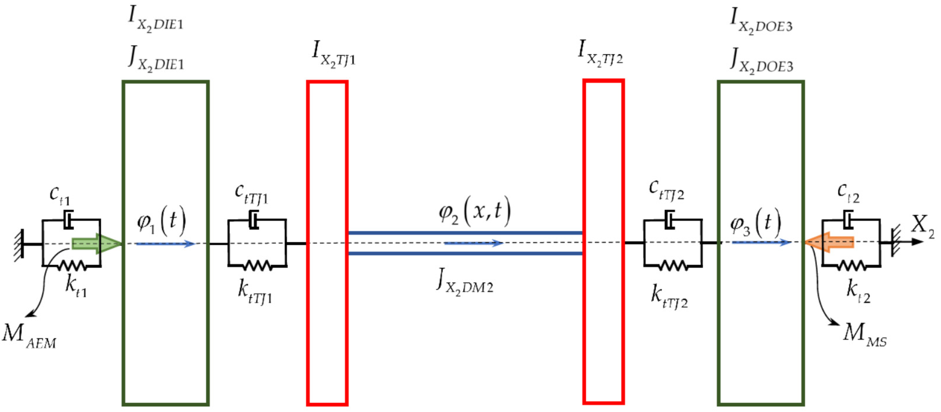The rigidity and the damping of the DTID’s elements are like those presented in [9] because the DTID also has three elements, DIE1, DME2, and DOE3, as illustrated in Figure 8, linked through the joints TJ1 (tripod joint 1) and TJ2 (tripod joint 2), with dynamic torsional characteristics expressed as follows:

• The first DTID element is DIE1 (see Figure 7 and Figure 8), which has the torsion rigidity and the torsion damping coefficient given by the equations:

$${\mathrm{k}}_{\mathrm{t}1}=\mathrm{G}\frac{{\mathrm{J}}_{{\mathrm{X}}_2\mathrm{A}1}{\mathrm{J}}_{{\mathrm{X}}_2\mathrm{B}1}}{{\mathrm{J}}_{{\mathrm{X}}_2\mathrm{A}1}{\mathrm{L}}_{\mathrm{B}1}+{\mathrm{J}}_{{\mathrm{X}}_2\mathrm{B}1}{\mathrm{L}}_{\mathrm{A}1}},{\mathrm{c}}_{\mathrm{t}1}=2\mathsf{\zeta }\sqrt{{\mathrm{k}}_{\mathrm{t}1}{\mathrm{I}}_{{\mathrm{X}}_2\mathrm{D}\mathrm{I}\mathrm{E}1}},$$

(1)

where G is the steel shear modulus, ${\mathrm{k}}_{\mathrm{t}1},{\mathrm{c}}_{\mathrm{t}1}$ are the stiffness and the damping coefficient in torsion of DIE1, and $\mathsf{\zeta }$ is the damping ratio of the DIE1’s material, steel, having the value range 0.0016–0.0318 [9];

2.

The TJ1 is the tripod that links DIE1 and DME2 (see Figure 7 and Figure 8), having the torsion stiffness ${\mathrm{k}}_{\mathrm{t}\mathrm{T}\mathrm{J}1}$ and the coefficient of torsion damping ${\mathrm{c}}_{\mathrm{t}\mathrm{T}\mathrm{J}1}$;

3.

The second DTID element is DME2 (see Figure 7 and Figure 8), which has a continuous elastic behavior in torsion and has fixed through splines at both ends of the tripods with the inertial characteristics in torsion

$${\mathrm{I}}_{{\mathrm{X}}_2\mathrm{T}\mathrm{J}1}={\mathrm{J}}_{{\mathrm{X}}_2\mathrm{T}1}\mathsf{\rho }{\mathrm{L}}_{\mathrm{T}1}=\left({\mathrm{J}}_{1\mathrm{T}1}+{\mathrm{J}}_{2\mathrm{T}1}+{\mathrm{J}}_{{\mathrm{X}}_2\mathrm{D}\mathrm{M}2}\right)\mathsf{\rho }{\mathrm{L}}_{\mathrm{T}1},$$

(2)

$${\mathrm{I}}_{{\mathrm{X}}_2\mathrm{T}\mathrm{J}2}={\mathrm{J}}_{{\mathrm{X}}_2\mathrm{T}2}\mathsf{\rho }{\mathrm{L}}_{\mathrm{T}2}=\left({\mathrm{J}}_{1\mathrm{T}2}+{\mathrm{J}}_{2\mathrm{T}2}+{\mathrm{J}}_{{\mathrm{X}}_2\mathrm{D}\mathrm{M}2}\right)\mathsf{\rho }{\mathrm{L}}_{\mathrm{T}2},$$

(3)

$${\mathrm{J}}_{{\mathrm{X}}_2\mathrm{D}\mathrm{M}2}=\frac{\pi {\mathrm{d}}_{\mathrm{D}\mathrm{M}2}^4}{32},$$

(4)

where ${\mathrm{I}}_{{\mathrm{X}}_2\mathrm{T}\mathrm{J}1},$ ${\mathrm{I}}_{{\mathrm{X}}_2\mathrm{T}\mathrm{J}2}$ are the axial mass moment of inertia of the tripods with the DME2’s axis included, ${\mathrm{I}}_{{\mathrm{X}}_2\mathrm{D}\mathrm{M}2}$ has the same signification for DME2, ${\mathrm{L}}_{\mathrm{T}1},$${\mathrm{L}}_{\mathrm{T}2}$ are the lengths of the tripods, and ${\mathrm{d}}_{\mathrm{D}\mathrm{M}2}$ is the diameter of the DTID’s element DME2;

4.

The TJ2 is the tripod that links DME2 and DOE3 (see Figure 7 and Figure 8), having the torsion stiffness ${\mathrm{k}}_{\mathrm{t}\mathrm{T}\mathrm{J}2}$ and the coefficient of torsion damping ${\mathrm{c}}_{\mathrm{t}\mathrm{T}\mathrm{J}2}$;

5.

The third DTID element is DOE3 (see Figure 7 and Figure 8), which has the torsion rigidity and the torsion damping coefficient given by the equations:

$${\mathrm{k}}_{\mathrm{t}2}=\mathrm{G}\frac{{\mathrm{J}}_{{\mathrm{X}}_2\mathrm{A}3}{\mathrm{J}}_{{\mathrm{X}}_2\mathrm{B}3}}{{\mathrm{J}}_{{\mathrm{X}}_2\mathrm{A}3}{\mathrm{L}}_{\mathrm{B}3}+{\mathrm{J}}_{{\mathrm{X}}_2\mathrm{B}3}{\mathrm{L}}_{\mathrm{A}3}},{\mathrm{c}}_{\mathrm{t}2}=2\mathsf{\zeta }\sqrt{{\mathrm{k}}_{\mathrm{t}2}{\mathrm{I}}_{{\mathrm{X}}_2\mathrm{D}\mathrm{O}\mathrm{E}3}},$$

(5)

where ${\mathrm{k}}_{\mathrm{t}2},{\mathrm{c}}_{\mathrm{t}2}$ are the stiffness and the damping coefficient in torsion of DOE3. The equation gives the load torque received by DTID from the asynchronous electric motor (see Figure 7 and Figure 8) [25,26]:

$${\mathrm{M}}_{\mathrm{A}\mathrm{E}\mathrm{M}}={\overline{\mathrm{M}}}_{\mathrm{A}\mathrm{E}\mathrm{M}}\left[1+{\chi }_{\mathrm{A}\mathrm{E}\mathrm{M}}{\displaystyle \sum _{\mathrm{i}=0}^5\frac{\cos \left(2^{\mathrm{i}}{\mathsf{\Omega }}_{\mathrm{A}\mathrm{E}\mathrm{M}}\mathrm{t}\right)}{2^{\mathrm{i}+1}}}\right],$$

(6)

$${\mathsf{\Omega }}_{\mathrm{A}\mathrm{E}\mathrm{M}}=\frac{\pi {\mathrm{n}}_{\mathrm{A}\mathrm{E}\mathrm{M}}}{30},$$

(7)

where ${\chi }_{\mathrm{A}\mathrm{E}\mathrm{M}}$ is the nonuniformity of the asynchronous electric motor torque, having the value in the field 0.01–0.07 [25], ${\overline{\mathrm{M}}}_{\mathrm{A}\mathrm{E}\mathrm{M}}$ is the amplitude of the engine torque in Nm, and ${\mathrm{n}}_{\mathrm{A}\mathrm{E}\mathrm{M}}$ is the output velocity angle of the asynchronous electric motor in rot/min. As mentioned in [25], due to the manifested nonuniformity instantaneous electromagnetic torque components in the range of −0.1–0.1 (manifestation that exists even for synchronous motor [26]), the active and reactive electric power has a nonuniformity in the range ±0.07 [25,26]. Therefore, the output torque has the same nonuniformity. Usually, these nonuniformities have a harmonic variation given by the equation [25]:

$${\mathsf{\Omega }}_{\mathrm{A}\mathrm{E}\mathrm{M}}=\frac{\pi {\mathrm{n}}_{\mathrm{A}\mathrm{E}\mathrm{M}}}{30}=100\mathrm{n}\pi ,\mathrm{n}=6,12,24,48,96.$$

(8)

A reactive torque charges the output element DOE3 of DTID due to the milling system (see Figure 7 and Figure 8), having a similar harmonic variation due to the variable granulation of the substance to mill as the input torque ${\mathrm{M}}_{\mathrm{A}\mathrm{E}\mathrm{M}}$, given by the equation:

$${\mathrm{M}}_{\mathrm{M}\mathrm{S}}={\overline{\mathrm{M}}}_{\mathrm{M}\mathrm{S}}\left[1+{\chi }_{\mathrm{M}\mathrm{S}}{\displaystyle \sum _{\mathrm{j}=1}^7\frac{\cos \left(2^{\mathrm{j}-1}{\mathsf{\phi }}_3\left(\mathrm{t}\right)\right)}{2^{\mathrm{j}}}}\right],$$

(9)

where ${\overline{\mathrm{M}}}_{\mathrm{M}\mathrm{S}}$ is the amplitude of reactive torque of the milling system and ${\chi }_{\mathrm{M}\mathrm{S}}$ is a moderate nonuniformity due to the granulation of the material milled in the system, having a value in the range 0–0.17 [27] (pp. 319–348). Analyzing the Equations (1)–(9) and the Figure 3, Figure 4, Figure 6, Figure 7 and Figure 8, it can be remarked that the PCM for FTV of the automotive driveshaft, presented in [9], was modified to overcome the reality, so for DTID, the new MPCM has two tripod joints instead of one, with different geometric characteristics and different inertia manifestation. Additionally, the new MPCM for FTV has multiple harmonic excitations terms, which is a generalization of double excitations terms as in [28,29] (p. 14), this being another novel aspect that this work has improved. This aspect of multiple excitation terms is a consequence of using an asynchronous electric motor as a power supplier (the best economic choice) and the various granulations of the milling substance.

3. The System Equations of Motion for Double Tripod Industrial Driveshaft’s FTV

For the MPCM of FTV for DTID (see Figure 8), considering the same mathematical procedure as in [9], Hamilton’s Principle, it yields the system equations of motion:

$${\mathrm{I}}_{{\mathrm{X}}_2\mathrm{D}\mathrm{I}\mathrm{E}1}({\mathsf{\phi }}_1){\ddot{\mathsf{\phi }}}_1+\left[{\mathrm{c}}_{\mathrm{t}1}+3{\mathrm{c}}_{\mathrm{t}\mathrm{T}\mathrm{J}1}{\mathrm{A}}_{\mathrm{T}\mathrm{J}1}\sin (3{\mathsf{\phi }}_1)\right]{\dot{\mathsf{\phi }}}_1+\left[{\mathrm{k}}_{\mathrm{t}1}-{\mathrm{k}}_{\mathrm{t}\mathrm{T}\mathrm{J}1}{\mathrm{A}}_{\mathrm{T}\mathrm{J}1}\cos (3{\mathsf{\phi }}_1)\right]{\mathsf{\phi }}_1={\overline{\mathrm{M}}}_{\mathrm{A}\mathrm{E}\mathrm{M}}\left[1+{\chi }_{\mathrm{A}\mathrm{E}\mathrm{M}}{\displaystyle \sum _{\mathrm{i}=0}^5\frac{\cos \left(2^{\mathrm{i}}{\mathsf{\Omega }}_{\mathrm{A}\mathrm{E}\mathrm{M}}\mathrm{t}\right)}{2^{\mathrm{i}+1}}}\right]\left(1-3{\mathrm{A}}_{\mathrm{T}\mathrm{J}1}\sin (3{\mathsf{\phi }}_1)\right),$$

(10)

$$\frac{{\partial }^2{\mathsf{\phi }}_2}{\partial {\mathrm{t}}^2}={\mathrm{c}}^2\frac{{\partial }^2{\mathsf{\phi }}_2}{\partial {\mathrm{x}}^2},\mathrm{c}=\sqrt{\frac{\mathrm{G}}{\mathsf{\rho }}},$$

(11)

$${\mathrm{I}}_{{\mathrm{X}}_2\mathrm{D}\mathrm{O}\mathrm{E}3}({\mathsf{\phi }}_3){\ddot{\mathsf{\phi }}}_3+\left[{\mathrm{c}}_{\mathrm{t}2}-3{\mathrm{c}}_{\mathrm{t}\mathrm{T}\mathrm{J}2}{\mathrm{A}}_{\mathrm{T}\mathrm{J}2}\sin (3{\mathsf{\phi }}_3)\right]{\dot{\mathsf{\phi }}}_3+\left[{\mathrm{k}}_{\mathrm{t}2}+{\mathrm{k}}_{\mathrm{t}\mathrm{T}\mathrm{J}2}{\mathrm{A}}_{\mathrm{T}\mathrm{J}2}\cos (3{\mathsf{\phi }}_3)\right]{\mathsf{\phi }}_3=-{\overline{\mathrm{M}}}_{\mathrm{M}\mathrm{S}}\left[1+{\chi }_{\mathrm{M}\mathrm{S}}{\displaystyle \sum _{\mathrm{j}=1}^7\frac{\cos \left(2^{\mathrm{j}-1}{\mathsf{\phi }}_3\left(\mathrm{t}\right)\right)}{2^{\mathrm{j}}}}\right]\left(1-3{\mathrm{A}}_{\mathrm{T}\mathrm{J}2}\sin (3{\mathsf{\phi }}_3)\right),$$

(12)

where ${\mathrm{A}}_{\mathrm{T}\mathrm{J}1},$ ${\mathrm{A}}_{\mathrm{T}\mathrm{J}2}$ are [1] (p. 78), [9]:

$${\mathrm{A}}_{\mathrm{T}\mathrm{J}1}=0.5\frac{{\mathrm{R}}_{\mathrm{T}\mathrm{J}1}}{{\mathrm{L}}_{\mathrm{D}\mathrm{M}2}}\tan {\mathsf{\beta }}_1{\tan }^2\frac{{\mathsf{\beta }}_1}{2},$$

(13)

$${\mathrm{A}}_{\mathrm{T}\mathrm{J}2}=0.5\frac{{\mathrm{R}}_{\mathrm{T}\mathrm{J}2}}{{\mathrm{L}}_{\mathrm{D}\mathrm{M}2}}\tan {\mathsf{\beta }}_2{\tan }^2\frac{{\mathsf{\beta }}_2}{2},$$

(14)

where ${\mathrm{L}}_{\mathrm{D}\mathrm{M}2}$ is the length of DME2 measured between the centroids of TJ1 and TJ2, ${\mathrm{R}}_{\mathrm{T}\mathrm{J}1},$ ${\mathrm{R}}_{\mathrm{T}\mathrm{J}2}$ are the geometrical radii of the tripods joints TJ1 and TJ2, and the boundary conditions of DTID are expressed by the equations:

$${\mathrm{I}}_{{\mathrm{X}}_2\mathrm{T}\mathrm{J}1}\frac{{\partial }^2{\mathsf{\phi }}_2\left(0,\mathrm{t}\right)}{\partial {\mathrm{t}}^2}-3{\mathrm{c}}_{\mathrm{t}\mathrm{T}\mathrm{J}1}{\mathrm{A}}_{\mathrm{T}\mathrm{J}1}\sin (3{\mathsf{\phi }}_1){\dot{\mathsf{\phi }}}_1+{\mathrm{k}}_{\mathrm{t}\mathrm{T}\mathrm{J}1}{\mathrm{A}}_{\mathrm{T}\mathrm{J}1}\cos (3{\mathsf{\phi }}_1){\mathsf{\phi }}_1-\mathrm{G}{\mathrm{J}}_{{\mathrm{X}}_2\mathrm{D}\mathrm{M}2}\frac{\partial {\mathsf{\phi }}_2(0,\mathrm{t})}{\partial \mathrm{x}}=0,\mathrm{a}\mathrm{t}\mathrm{x}=0,$$

(15)

$${\mathrm{I}}_{{\mathrm{X}}_2\mathrm{T}\mathrm{J}2}\frac{{\partial }^2{\mathsf{\phi }}_2\left({\mathrm{L}}_{\mathrm{D}\mathrm{M}2},\mathrm{t}\right)}{\partial {\mathrm{t}}^2}+3{\mathrm{c}}_{\mathrm{t}\mathrm{T}\mathrm{J}2}{\mathrm{A}}_{\mathrm{T}\mathrm{J}2}\sin (3{\mathsf{\phi }}_3){\dot{\mathsf{\phi }}}_3-{\mathrm{k}}_{\mathrm{t}\mathrm{T}\mathrm{J}2}{\mathrm{A}}_{\mathrm{T}\mathrm{J}2}\cos (3{\mathsf{\phi }}_3){\mathsf{\phi }}_3+\mathrm{G}{\mathrm{J}}_{{\mathrm{X}}_2\mathrm{D}\mathrm{M}2}\frac{\partial {\mathsf{\phi }}_2({\mathrm{L}}_{\mathrm{D}\mathrm{M}2},\mathrm{t})}{\partial \mathrm{x}}=0,\mathrm{a}\mathrm{t}\mathrm{x}={\mathrm{L}}_{\mathrm{D}\mathrm{M}2}.$$

(16)

The system of Equations (SEs) (10)–(12) coupled with the Equations (13) and (14) and the boundary conditions (15) and (16) expressed the nonlinear dynamic behavior of FTV for DTID excited by an input harmonic torque generated by an asynchronous electric motor and having an output harmonic excitation caused by the granulation of materials needed to be milled. Equations (13) and (14) represent the geometric and kinematic nonuniformity of DTID generated by the effect that the tripod’s joints are quasi-homokinetic [1,2,3]. In close regard, it is evident that Equations (10) and (12) are the equations of forced torsional parametric vibrations of DIE1 and DOE3 representing modified Mathieu–Hill equations; in contrast, (11) is a differential equation for the vibrations of a uniform shaft in torsion. The DME2 has fixed–fixed boundary conditions in torsion, and therefore, the solution of Equation (11) yields:

$${\mathsf{\phi }}_2(\mathrm{x},\mathrm{t})={\displaystyle \sum _{\mathrm{k}=1}^{\infty }{\mathrm{A}}_{\mathrm{k}}\cos \left(\frac{{\mathsf{\omega }}_{\mathrm{k}}\mathrm{x}}{\mathrm{c}}-{\mathsf{\delta }}_{1\mathrm{k}}\right)\cos \left({\mathsf{\omega }}_{\mathrm{k}}\mathrm{t}-{\mathsf{\delta }}_{2\mathrm{k}}\right)},{\mathsf{\omega }}_{\mathrm{k}}=\frac{\mathrm{k}\pi \mathrm{c}}{{\mathrm{L}}_{\mathrm{D}\mathrm{M}2}},\mathrm{k}=1,2,3,\dots$$

(17)

where ${\mathrm{A}}_{\mathrm{k}}$ represents the amplitude in torsion of DME2, ${\mathsf{\delta }}_{1\mathrm{k}},{\mathsf{\delta }}_{2\mathrm{k}}$ are the phase’s angles, and ${\mathsf{\omega }}_{\mathrm{k}}$ is the natural pulsation (NP) of the free vibrations in torsion of the DME2. Injecting the Equation (17) into the boundary conditions (15) and (16) yields:

$$\begin{array}{l}-3{\mathrm{c}}_{\mathrm{t}\mathrm{T}\mathrm{J}1}{\mathrm{A}}_{\mathrm{T}\mathrm{J}1}\sin (3{\mathsf{\phi }}_1){\dot{\mathsf{\phi }}}_1+{\mathrm{k}}_{\mathrm{t}\mathrm{T}\mathrm{J}1}{\mathrm{A}}_{\mathrm{T}\mathrm{J}1}\cos (3{\mathsf{\phi }}_1){\mathsf{\phi }}_1=-{\mathrm{I}}_{{\mathrm{X}}_2\mathrm{T}\mathrm{J}1}\frac{{\partial }^2{\mathsf{\phi }}_2\left(0,\mathrm{t}\right)}{\partial {\mathrm{t}}^2}+\mathrm{G}{\mathrm{J}}_{{\mathrm{X}}_2\mathrm{D}\mathrm{M}2}\frac{\partial {\mathsf{\phi }}_2(0,\mathrm{t})}{\partial \mathrm{x}}\\ ={\displaystyle \sum _{\mathrm{k}=1}^{\infty }{\mathrm{A}}_{\mathrm{k}}\left[{\mathrm{I}}_{{\mathrm{X}}_2\mathrm{T}\mathrm{J}1}{\mathsf{\omega }}_{\mathrm{k}}^2\cos {\mathsf{\delta }}_{1\mathrm{k}}+\mathrm{G}{\mathrm{J}}_{{\mathrm{X}}_2\mathrm{D}\mathrm{M}2}\frac{{\mathsf{\omega }}_{\mathrm{k}}}{\mathrm{c}}\sin {\mathsf{\delta }}_{1\mathrm{k}}\right]}\cos \left({\mathsf{\omega }}_{\mathrm{k}}\mathrm{t}-{\mathsf{\delta }}_{2\mathrm{k}}\right),\mathrm{a}\mathrm{t}\mathrm{x}=0,\end{array}$$

(18)

$$\begin{array}{l}3{\mathrm{c}}_{\mathrm{t}\mathrm{T}\mathrm{J}2}{\mathrm{A}}_{\mathrm{T}\mathrm{J}2}\sin (3{\mathsf{\phi }}_3){\dot{\mathsf{\phi }}}_3-{\mathrm{k}}_{\mathrm{t}\mathrm{T}\mathrm{J}2}{\mathrm{A}}_{\mathrm{T}\mathrm{J}2}\cos (3{\mathsf{\phi }}_3){\mathsf{\phi }}_3+=-{\mathrm{I}}_{{\mathrm{X}}_2\mathrm{T}\mathrm{J}2}\frac{{\partial }^2{\mathsf{\phi }}_2\left({\mathrm{L}}_{\mathrm{D}\mathrm{M}2},\mathrm{t}\right)}{\partial {\mathrm{t}}^2}-\mathrm{G}{\mathrm{J}}_{{\mathrm{X}}_2\mathrm{D}\mathrm{M}2}\frac{\partial {\mathsf{\phi }}_2({\mathrm{L}}_{\mathrm{D}\mathrm{M}2},\mathrm{t})}{\partial \mathrm{x}}\\ ={\displaystyle \sum _{\mathrm{k}=1}^{\infty }{\mathrm{A}}_{\mathrm{k}}\left[{\mathrm{I}}_{{\mathrm{X}}_2\mathrm{T}\mathrm{J}2}{\mathsf{\omega }}_{\mathrm{k}}^2\cos \left(\frac{{\mathsf{\omega }}_{\mathrm{k}}{\mathrm{L}}_{\mathrm{D}\mathrm{M}2}}{\mathrm{c}}-{\mathsf{\delta }}_{1\mathrm{k}}\right)-\mathrm{G}{\mathrm{J}}_{{\mathrm{X}}_2\mathrm{D}\mathrm{M}2}\frac{{\mathsf{\omega }}_{\mathrm{k}}}{\mathrm{c}}\sin \left(\frac{{\mathsf{\omega }}_{\mathrm{k}}{\mathrm{L}}_{\mathrm{D}\mathrm{M}2}}{\mathrm{c}}-{\mathsf{\delta }}_{1\mathrm{k}}\right)\right]}\cos \left({\mathsf{\omega }}_{\mathrm{k}}\mathrm{t}-{\mathsf{\delta }}_{2\mathrm{k}}\right),\mathrm{a}\mathrm{t}\mathrm{x}={\mathrm{L}}_{\mathrm{D}\mathrm{M}2}.\end{array}$$

(19)

Using the mathematical expression (18) into (10) and the mathematical expression (19) into (12), the equations of FTV for DTID’s DIE1 and DOE3 are:

$$\begin{array}{l}{\ddot{\mathsf{\phi }}}_1+2\mathsf{\zeta }{\mathsf{\Omega }}_1\sqrt{\frac{1+{\mathrm{c}}_1\cos 2{\mathsf{\phi }}_1}{\left(1+{\mathrm{c}}_2\cos 2{\mathsf{\phi }}_1\right)\left(1+{\chi }_{\mathrm{n}\mathrm{D}\mathrm{I}\mathrm{E}1}\cos 2{\mathsf{\phi }}_1\right)}}{\dot{\mathsf{\phi }}}_1+{\mathsf{\Omega }}_1^2\frac{1+{\mathrm{c}}_1\cos 2{\mathsf{\phi }}_1}{\left(1+{\mathrm{c}}_2\cos 2{\mathsf{\phi }}_1\right)\left(1+{\chi }_{\mathrm{n}\mathrm{D}\mathrm{I}\mathrm{E}1}\cos 2{\mathsf{\phi }}_1\right)}{\mathsf{\phi }}_1=\frac{{\overline{\mathrm{M}}}_{\mathrm{A}\mathrm{E}\mathrm{M}}}{{\overline{\mathrm{I}}}_{{\mathrm{X}}_2\mathrm{D}\mathrm{I}\mathrm{E}1}}\frac{1+{\chi }_{\mathrm{A}\mathrm{E}\mathrm{M}}{\displaystyle \sum _{\mathrm{i}=0}^5\frac{\cos \left(2^{\mathrm{i}}{\mathsf{\Omega }}_{\mathrm{A}\mathrm{E}\mathrm{M}}\mathrm{t}\right)}{2^{\mathrm{i}+1}}}}{\left(1+{\chi }_{\mathrm{n}\mathrm{D}\mathrm{I}\mathrm{E}1}\cos 2{\mathsf{\phi }}_1\right)}\left(1-3{\mathrm{A}}_{\mathrm{T}\mathrm{J}1}\sin 3{\mathsf{\phi }}_1\right)\\ +{\displaystyle \sum _{\mathrm{k}=1}^{\infty }{\mathrm{A}}_{\mathrm{k}}\left[\frac{{\mathrm{I}}_{\mathrm{T}\mathrm{J}1}}{{\overline{\mathrm{I}}}_{{\mathrm{X}}_2\mathrm{D}\mathrm{I}\mathrm{E}1}}{\mathsf{\omega }}_{\mathrm{k}}^2\cos {\mathsf{\delta }}_{1\mathrm{k}}+\frac{\mathrm{G}{\mathrm{J}}_{{\mathrm{X}}_2\mathrm{D}\mathrm{M}2}}{{\overline{\mathrm{I}}}_{{\mathrm{X}}_2\mathrm{D}\mathrm{I}\mathrm{E}1}}\frac{{\mathsf{\omega }}_{\mathrm{k}}}{\mathrm{c}}\sin {\mathsf{\delta }}_{1\mathrm{k}}\right]\frac{\cos \left({\mathsf{\omega }}_{\mathrm{k}}\mathrm{t}-{\mathsf{\delta }}_{2\mathrm{k}}\right)}{\left(1+{\chi }_{\mathrm{n}\mathrm{D}\mathrm{I}\mathrm{E}1}\cos 2{\mathsf{\phi }}_1\right)}},\end{array}$$

(20)

$$\begin{array}{l}{\ddot{\mathsf{\phi }}}_3+2\mathsf{\zeta }{\mathsf{\Omega }}_3\sqrt{\frac{1+{\mathrm{c}}_3\cos 2{\mathsf{\phi }}_3}{\left(1+{\mathrm{c}}_4\cos 2{\mathsf{\phi }}_3\right)\left(1+{\chi }_{\mathrm{n}\mathrm{D}\mathrm{O}\mathrm{E}3}\cos 2{\mathsf{\phi }}_3\right)}}{\dot{\mathsf{\phi }}}_3+{\mathsf{\Omega }}_3^2\frac{1+{\mathrm{c}}_3\cos 2{\mathsf{\phi }}_3}{\left(1+{\mathrm{c}}_4\cos 2{\mathsf{\phi }}_3\right)\left(1+{\chi }_{\mathrm{n}\mathrm{D}\mathrm{O}\mathrm{E}3}\cos 2{\mathsf{\phi }}_3\right)}{\mathsf{\phi }}_3=-\frac{{\mathrm{M}}_{\mathrm{M}\mathrm{S}}}{{\overline{\mathrm{I}}}_{{\mathrm{X}}_2\mathrm{D}\mathrm{O}\mathrm{E}3}}\frac{1+{\chi }_{\mathrm{M}\mathrm{S}}{\displaystyle \sum _{\mathrm{j}=1}^7\frac{\cos \left(2^{\mathrm{j}-1}{\mathsf{\phi }}_3\left(\mathrm{t}\right)\right)}{2^{\mathrm{j}}}}}{\left(1+{\chi }_{\mathrm{n}\mathrm{D}\mathrm{O}\mathrm{E}3}\cos 2{\mathsf{\phi }}_3\right)}\left(1-3{\mathrm{A}}_{\mathrm{T}\mathrm{J}2}\sin 3{\mathsf{\phi }}_3\right)\\ +{\displaystyle \sum _{\mathrm{k}=1}^{\infty }{\left(-1\right)}^{\mathrm{k}}{\mathrm{A}}_{\mathrm{k}}\left[\frac{{\mathrm{I}}_{\mathrm{T}\mathrm{J}2}}{{\overline{\mathrm{I}}}_{{\mathrm{X}}_2\mathrm{D}\mathrm{O}\mathrm{E}3}}{\mathsf{\omega }}_{\mathrm{k}}^2\cos {\mathsf{\delta }}_{1\mathrm{k}}+\frac{\mathrm{G}{\mathrm{J}}_{{\mathrm{X}}_2\mathrm{D}\mathrm{M}2}}{{\overline{\mathrm{I}}}_{{\mathrm{X}}_2\mathrm{D}\mathrm{O}\mathrm{E}3}}\frac{{\mathsf{\omega }}_{\mathrm{k}}}{\mathrm{c}}\sin {\mathsf{\delta }}_{1\mathrm{k}}\right]\frac{\cos \left({\mathsf{\omega }}_{\mathrm{k}}\mathrm{t}-{\mathsf{\delta }}_{2\mathrm{k}}\right)}{\left(1+{\chi }_{\mathrm{n}\mathrm{D}\mathrm{O}\mathrm{E}3}\cos 2{\mathsf{\phi }}_3\right)},}\end{array}$$

(21)

where ${\mathsf{\Omega }}_1,{\mathsf{\Omega }}_3$ are the NP of DIE1 and DOE3, expressed by the equations:

$${\mathsf{\Omega }}_1=\frac{\mathrm{c}}{{\mathrm{L}}_{\mathrm{B}1}}{\left[\frac{1-\frac{{\mathrm{J}}_{{\mathrm{X}}_2\mathrm{A}1}\mathsf{\rho }{\mathrm{L}}_{\mathrm{A}1}}{{\overline{\mathrm{I}}}_{{\mathrm{X}}_2\mathrm{D}\mathrm{I}\mathrm{E}1}}}{1+{\left(\frac{{\mathrm{L}}_{\mathrm{A}1}}{{\mathrm{L}}_{\mathrm{B}1}}\right)}^2\left(\frac{{\overline{\mathrm{I}}}_{{\mathrm{X}}_2\mathrm{D}\mathrm{I}\mathrm{E}1}}{{\mathrm{J}}_{{\mathrm{X}}_2\mathrm{A}1}\mathsf{\rho }{\mathrm{L}}_{\mathrm{A}1}}-1\right)}\right]}^{1/2},$$

(22)

$${\mathsf{\Omega }}_3=\frac{\mathrm{c}}{{\mathrm{L}}_{\mathrm{B}3}}{\left[\frac{1-\frac{{\mathrm{J}}_{{\mathrm{X}}_2\mathrm{A}3}\mathsf{\rho }{\mathrm{L}}_{\mathrm{A}3}}{{\overline{\mathrm{I}}}_{{\mathrm{X}}_2\mathrm{D}\mathrm{O}\mathrm{E}3}}}{1+{\left(\frac{{\mathrm{L}}_{\mathrm{A}3}}{{\mathrm{L}}_{\mathrm{B}3}}\right)}^2\left(\frac{{\overline{\mathrm{I}}}_{{\mathrm{X}}_2\mathrm{D}\mathrm{O}\mathrm{E}3}}{{\mathrm{J}}_{{\mathrm{X}}_2\mathrm{A}3}\mathsf{\rho }{\mathrm{L}}_{\mathrm{A}3}}-1\right)}\right]}^{1/2},$$

(23)

${\chi }_{\mathrm{n}\mathrm{D}\mathrm{I}\mathrm{E}1},{\chi }_{\mathrm{n}\mathrm{D}\mathrm{O}\mathrm{E}3}$ are the geometric nonuniformities of DIE1 and DOE3 (see Appendix B), ${\overline{\mathrm{I}}}_{{\mathrm{X}}_2\mathrm{D}\mathrm{I}\mathrm{E}1}$ and ${\overline{\mathrm{I}}}_{{\mathrm{X}}_2\mathrm{D}\mathrm{O}\mathrm{E}3}$ are the AMMIs of DIE1 and DOE3 for ${\mathsf{\beta }}_1=0,{\mathsf{\beta }}_2=0$, and the coefficients ${\mathrm{c}}_{\mathrm{i}},\mathrm{i}=1,2,3,4$ are presented in Appendix B. The SEs (20) and (21) are generalized Mathieu–Hill coupled due to excitation $\cos ({\mathsf{\omega }}_{\mathrm{k}}\mathrm{t}\pm {\mathsf{\delta }}_{\mathrm{k}})$. The form of the SEs (20) and (21) contains parametric coefficients indicating specific resonances regions. As mentioned in [29] (p. 425), one of the most important resonance regions is the PPRR for excitation frequencies ${\mathsf{\eta }}_1\simeq 2{\mathsf{\Omega }}_1,{\mathsf{\eta }}_3\simeq 2{\mathsf{\Omega }}_3.$ The following paragraph will investigate the chaotic manifestation for NFTV of DIE1 and DOE3, expressed by the SEs (20) and (21), using time–history analysis in PPRR.

4. Detection of Chaotic Manifestation for Nonstationary FTV of Double Tripod Industrial Driveshaft in Principal Parametric Resonance Region

To detect chaotic manifestation for NFTV of DTID in PPRR, the Equations (20) and (21) are used to compute the phase portrait graphs $\left({\mathsf{\phi }}_1,\frac{\mathrm{d}{\mathsf{\phi }}_1}{\mathrm{d}\mathrm{t}}\right),$ for DIE1 and DOE3 in PPRR. The DTID’s elements DIE1 and DOE3 considered to have the characteristics of the DTID’s material, the geometry characteristics such as the AGMIs, and their nonuniformity, are presented in

Table 1. Material and Geometry characteristics of DIE1 and TJ1.

$\mathsf{\rho }$ [kg/m3]	G [GPa]	Torsional Rigidity [Nm/rad]	$\mathsf{\zeta }$	LB1 [m]	LA1 [m]	LDM2 [m]	RTJ1 [m]	dA1 [m]	dCB1 [m]	SB1 [m2]	0.5 (J1B1 + J2B1) [m4]	${\chi }_{\mathrm{n}\mathrm{B}1}$
7850	77.3	1.11·104	1.6…31.8·10−3	0.190	0.130	0.940	0.070	0.054	0.098	0.0076	1.4645·10−5	0.22

and

Table 2. Material and Geometry characteristics of DOE3 and TJ2.

$\mathsf{\rho }$ [kg/m3]	G [GPa]	Torsional Rigidity [Nm/rad]	$\mathsf{\zeta }$	LB3 [m]	LA3 [m]	RTJ2 [m]	dA3 [m]	dCB3 [m]	SB3 [m2]	0.5(J1B3 + J2B3) [m4]	${\chi }_{\mathrm{n}\mathrm{B}3}$
7850	77.3	1.11·104	1.6…31.8·10−3	0.209	0.143	0.077	0.059	0.108	0.0092	2.1442·10−5	0.24

. These given geometric features are in agreement with those considered by Steinwede [18] (p. 111).

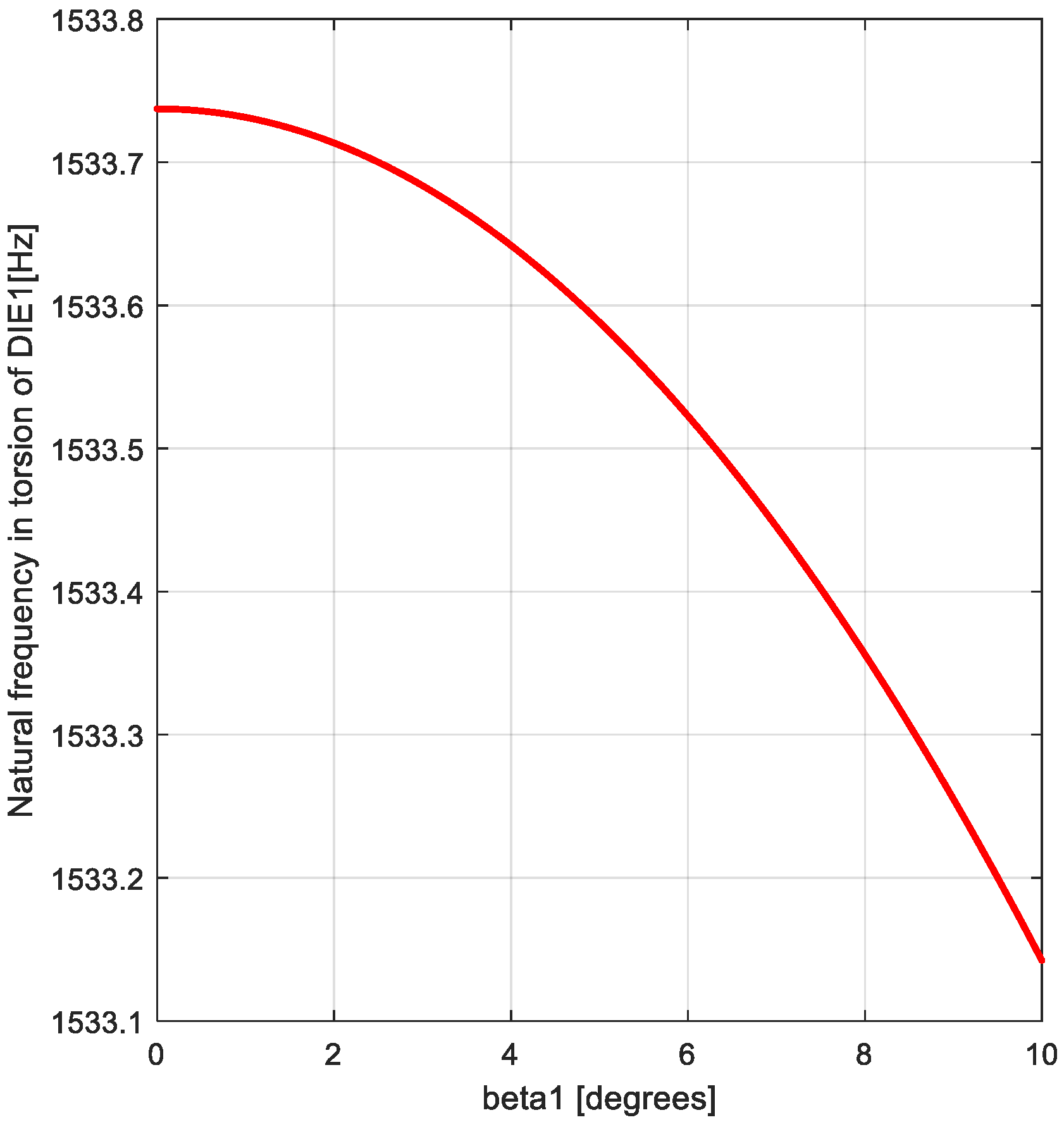
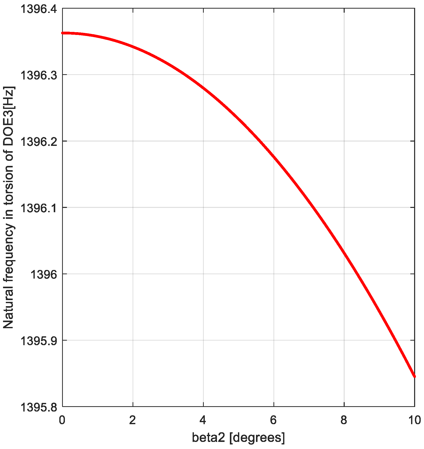
Based on AUTOCAD, ${\mathrm{J}}_{1\mathrm{B}1},{\mathrm{J}}_{2\mathrm{B}1},{\mathrm{J}}_{1\mathrm{B}3},{\mathrm{J}}_{2\mathrm{B}3}$ were calculated using the generic dimensions of the DTID’s DIE1 and DOE3. MATLAB software determined the variation graph of the functions ${\mathsf{\Omega }}_1\left({\mathsf{\beta }}_1\right),{\mathsf{\Omega }}_3\left({\mathsf{\beta }}_2\right)$, representing the NPs of DIE1 and DOE3 as presented in Figure 9 and Figure 10.

The values obtained for NPs of DIE1 and DOE3, shown in the graphs presented in Figure 9 and Figure 10, agree with the values mentioned in [18] (pp. 119–139). Therefore, the MPCM of NFTV for DTID, which is a novelty of the present work, represents a model that agrees with the data in the literature [18].

Table 3. Natural frequencies in torsion for DM2.

Order	${\mathsf{\nu }}_{\mathrm{k}}$ [Hz]
1	1669.2
2	3338.4
3	5007.6
4	6676.8
5	8346

presents the free natural frequencies for the torsional vibrations of DME2 based on the Equation (17), yielding:

$${\mathsf{\nu }}_{\mathrm{k}}=\frac{{\mathsf{\omega }}_{\mathrm{k}}}{2\pi }=\frac{\mathrm{k}\mathrm{c}}{2{\mathrm{L}}_{\mathrm{D}\mathrm{M}2}}=\frac{\mathrm{k}\sqrt{\frac{\mathrm{G}}{\mathsf{\rho }}}}{2{\mathrm{L}}_{\mathrm{D}\mathrm{M}2}},\mathrm{k}=1,2,3,\dots$$

(24)

The last terms in Equations (20) and (21) are neglected because the excitation frequency in PPRR for DIE1 (see Figure 9) and for DOE3 (see Figure 10) is not in the range of free natural frequencies for torsional vibrations of DME2 (see Table 3) yielding the equations:

$${\ddot{\mathsf{\phi }}}_1+2\mathsf{\zeta }{\mathsf{\Omega }}_1\sqrt{\frac{1+{\mathrm{c}}_1\cos 2{\mathsf{\phi }}_1}{\left(1+{\mathrm{c}}_2\cos 2{\mathsf{\phi }}_1\right)\left(1+{\chi }_{\mathrm{n}\mathrm{D}\mathrm{I}\mathrm{E}1}\cos 2{\mathsf{\phi }}_1\right)}}{\dot{\mathsf{\phi }}}_1+{\mathsf{\Omega }}_1^2\frac{1+{\mathrm{c}}_1\cos 2{\mathsf{\phi }}_1}{\left(1+{\mathrm{c}}_2\cos 2{\mathsf{\phi }}_1\right)\left(1+{\chi }_{\mathrm{n}\mathrm{D}\mathrm{I}\mathrm{E}1}\cos 2{\mathsf{\phi }}_1\right)}{\mathsf{\phi }}_1=\frac{{\overline{\mathrm{M}}}_{\mathrm{A}\mathrm{E}\mathrm{M}}}{{\overline{\mathrm{I}}}_{{\mathrm{X}}_2\mathrm{D}\mathrm{I}\mathrm{E}1}}\frac{1+{\chi }_{\mathrm{A}\mathrm{E}\mathrm{M}}{\displaystyle \sum _{\mathrm{i}=0}^5\frac{\cos \left(2^{\mathrm{i}}{\mathsf{\Omega }}_{\mathrm{A}\mathrm{E}\mathrm{M}}\mathrm{t}\right)}{2^{\mathrm{i}+1}}}}{\left(1+{\chi }_{\mathrm{n}\mathrm{D}\mathrm{I}\mathrm{E}1}\cos 2{\mathsf{\phi }}_1\right)}\left(1-3{\mathrm{A}}_{\mathrm{T}\mathrm{J}1}\sin 3{\mathsf{\phi }}_1\right),$$

(25)

$${\ddot{\mathsf{\phi }}}_3+2\mathsf{\zeta }{\mathsf{\Omega }}_3\sqrt{\frac{1+{\mathrm{c}}_3\cos 2{\mathsf{\phi }}_3}{\left(1+{\mathrm{c}}_4\cos 2{\mathsf{\phi }}_3\right)\left(1+{\chi }_{\mathrm{n}\mathrm{D}\mathrm{O}\mathrm{E}3}\cos 2{\mathsf{\phi }}_3\right)}}{\dot{\mathsf{\phi }}}_3+{\mathsf{\Omega }}_3^2\frac{1+{\mathrm{c}}_3\cos 2{\mathsf{\phi }}_3}{\left(1+{\mathrm{c}}_4\cos 2{\mathsf{\phi }}_3\right)\left(1+{\chi }_{\mathrm{n}\mathrm{D}\mathrm{O}\mathrm{E}3}\cos 2{\mathsf{\phi }}_3\right)}{\mathsf{\phi }}_3=-\frac{{\mathrm{M}}_{\mathrm{M}\mathrm{S}}}{{\overline{\mathrm{I}}}_{{\mathrm{X}}_2\mathrm{D}\mathrm{O}\mathrm{E}3}}\frac{1+{\chi }_{\mathrm{M}\mathrm{S}}{\displaystyle \sum _{\mathrm{j}=1}^7\frac{\cos \left(2^{\mathrm{j}-1}{\mathsf{\phi }}_3\left(\mathrm{t}\right)\right)}{2^{\mathrm{j}}}}}{\left(1+{\chi }_{\mathrm{n}\mathrm{D}\mathrm{O}\mathrm{E}3}\cos 2{\mathsf{\phi }}_3\right)}\left(1-3{\mathrm{A}}_{\mathrm{T}\mathrm{J}2}\sin 3{\mathsf{\phi }}_3\right).$$

(26)

The characteristics of external excitations of DTID are presented in

Table 4. Characteristics of external excitations of DTID.

${\overline{\mathrm{M}}}_{\mathrm{A}\mathrm{E}\mathrm{M}}$ [kN·m]	${\overline{\mathrm{M}}}_{\mathrm{M}\mathrm{S}}$ [kN·m]	${\chi }_{\mathrm{A}\mathrm{E}\mathrm{M}}$	${\chi }_{\mathrm{M}\mathrm{S}}$
2.55	2.1	0.05	0.15

.

The expressions must define the excitation frequencies ${\mathsf{\eta }}_1,{\mathsf{\eta }}_3$ of DTID’s DIE1 and DOE3 in the PPRR:

$${\mathsf{\eta }}_1=\frac{2\mathrm{d}{\mathsf{\phi }}_1}{\mathrm{d}\mathrm{t}}\simeq 2{\mathsf{\Omega }}_1,$$

(27)

$${\mathsf{\eta }}_3=\frac{2\mathrm{d}{\mathsf{\phi }}_3}{\mathrm{d}\mathrm{t}}\simeq 2{\mathsf{\Omega }}_3.$$

(28)

To calculate the time–history graphs $\left({\mathsf{\phi }}_1(\mathrm{t}),\mathrm{t}\right),(\frac{\mathrm{d}{\mathsf{\phi }}_1}{\mathrm{d}\mathrm{t}}(\mathrm{t}),\mathrm{t}),\left({\mathsf{\phi }}_1(\mathrm{t}),\frac{\mathrm{d}{\mathsf{\phi }}_1}{\mathrm{d}\mathrm{t}}(\mathrm{t}),\mathrm{t}\right),\left({\mathsf{\phi }}_1(\mathrm{t}),\frac{\mathrm{d}{\mathsf{\phi }}_1}{\mathrm{d}\mathrm{t}}(\mathrm{t})\right)$ for DIE1 and $\left({\mathsf{\phi }}_3(\mathrm{t}),\mathrm{t}\right),(\frac{\mathrm{d}{\mathsf{\phi }}_3}{\mathrm{d}\mathrm{t}}(\mathrm{t}),\mathrm{t}),\left({\mathsf{\phi }}_3(\mathrm{t}),\frac{\mathrm{d}{\mathsf{\phi }}_3}{\mathrm{d}\mathrm{t}}(\mathrm{t}),\mathrm{t}\right),\left({\mathsf{\phi }}_3(\mathrm{t}),\frac{\mathrm{d}{\mathsf{\phi }}_3}{\mathrm{d}\mathrm{t}}(\mathrm{t})\right)$ for DOE3, the Equations (25) and (26) were numerically integrated using MATLAB software based on function ode 45 (Runge–Kutta integration method of fifth-order). The graphs $\left({\mathsf{\phi }}_1(\mathrm{t}),\frac{\mathrm{d}{\mathsf{\phi }}_1}{\mathrm{d}\mathrm{t}}(\mathrm{t})\right),$ $\left({\mathsf{\phi }}_3(\mathrm{t}),\frac{\mathrm{d}{\mathsf{\phi }}_3}{\mathrm{d}\mathrm{t}}(\mathrm{t})\right)$ represent the phase portraits of NFTV for DIE1 and DOE3, being the detection method of possible chaotic dynamic behavior. To certify the chaotic dynamic behavior of NFTV, the new robust method LEA–PM, described in the next paragraph, is used.

5. Chaotic Dynamic Analysis for Nonstationary FTV of Double Tripod Industrial Driveshaft in Principal Parametric Resonance Region

Suppose it is detected as a manifestation of chaotic dynamic behavior, such as specific chaotic orbits of the trajectories of the phase portraits for NFTV of DIE1, DOE3, or for both elements of DTID from the analysis of dynamic transition through PPRR. If this is the case, the existence of chaos needs to be certified using a robust method. First, the hypothesis of transition through PPRR is still valid. Considering that the relations (27) and (28) must be valid, for the excitation frequencies ${\mathsf{\eta }}_1,{\mathsf{\eta }}_3$ of DTID’s DIE1 and DOE3 in the PPRR, the Equations (25) and (26) must be put in the systemic mathematical form:

$$\{\begin{array}{c}\frac{\mathrm{d}{\mathsf{\phi }}_1}{\mathrm{d}\mathrm{t}}={\mathrm{V}}_{\mathsf{\phi }1},\\ \frac{\mathrm{d}{\mathsf{\Theta }}_1}{\mathrm{d}\mathrm{t}}={\mathsf{\eta }}_1,\\ \frac{\mathrm{d}{\mathrm{V}}_{\mathsf{\phi }1}}{\mathrm{d}\mathrm{t}}=-2\mathsf{\zeta }{\mathsf{\Omega }}_1\sqrt{\frac{1+{\mathrm{c}}_1\cos {\mathsf{\Theta }}_1}{\left(1+{\mathrm{c}}_2\cos {\mathsf{\Theta }}_1\right)\left(1+{\chi }_{\mathrm{n}\mathrm{D}\mathrm{I}\mathrm{E}1}\cos {\mathsf{\Theta }}_1\right)}}{\mathrm{V}}_{\mathsf{\phi }1}-{\mathsf{\Omega }}_1^2\frac{1+{\mathrm{c}}_1\cos {\mathsf{\Theta }}_1}{\left(1+{\mathrm{c}}_2\cos {\mathsf{\Theta }}_1\right)\left(1+{\chi }_{\mathrm{n}\mathrm{D}\mathrm{I}\mathrm{E}1}\cos {\mathsf{\Theta }}_1\right)}{\mathsf{\phi }}_1+\frac{{\overline{\mathrm{M}}}_{\mathrm{A}\mathrm{E}\mathrm{M}}}{{\overline{\mathrm{I}}}_{{\mathrm{X}}_2\mathrm{D}\mathrm{I}\mathrm{E}1}}\frac{1+{\chi }_{\mathrm{A}\mathrm{E}\mathrm{M}}{\displaystyle \sum _{\mathrm{i}=0}^5\frac{\cos \left(2^{\mathrm{i}}{\mathsf{\Omega }}_{\mathrm{A}\mathrm{E}\mathrm{M}}\mathrm{t}\right)}{2^{\mathrm{i}+1}}}}{\left(1+{\chi }_{\mathrm{n}\mathrm{D}\mathrm{I}\mathrm{E}1}\cos 2{\mathsf{\phi }}_1\right)}\left(1-3{\mathrm{A}}_{\mathrm{T}\mathrm{J}1}\sin 3{\mathsf{\phi }}_1\right),\end{array}$$

(29)

$$\{\begin{array}{c}\frac{\mathrm{d}{\mathsf{\phi }}_3}{\mathrm{d}\mathrm{t}}={\mathrm{V}}_{\mathsf{\phi }3},\\ \frac{\mathrm{d}{\mathsf{\Theta }}_3}{\mathrm{d}\mathrm{t}}={\mathsf{\eta }}_3,\\ \frac{\mathrm{d}{\mathrm{V}}_{\mathsf{\phi }3}}{\mathrm{d}\mathrm{t}}=-2\mathsf{\zeta }{\mathsf{\Omega }}_3\sqrt{\frac{1+{\mathrm{c}}_3\cos {\mathsf{\Theta }}_3}{\left(1+{\mathrm{c}}_4\cos {\mathsf{\Theta }}_1\right)\left(1+{\chi }_{\mathrm{n}\mathrm{D}\mathrm{O}\mathrm{E}3}\cos {\mathsf{\Theta }}_3\right)}}{\mathrm{V}}_{\mathsf{\phi }3}-{\mathsf{\Omega }}_3^2\frac{1+{\mathrm{c}}_3\cos {\mathsf{\Theta }}_3}{\left(1+{\mathrm{c}}_4\cos {\mathsf{\Theta }}_3\right)\left(1+{\chi }_{\mathrm{n}\mathrm{D}\mathrm{O}\mathrm{E}3}\cos {\mathsf{\Theta }}_3\right)}{\mathsf{\phi }}_3-\frac{{\mathrm{M}}_{\mathrm{M}\mathrm{S}}}{{\overline{\mathrm{I}}}_{{\mathrm{X}}_2\mathrm{D}\mathrm{O}\mathrm{E}3}}\frac{1+{\chi }_{\mathrm{M}\mathrm{S}}{\displaystyle \sum _{\mathrm{j}=1}^7\frac{\cos \left(2^{\mathrm{j}-1}{\mathsf{\phi }}_3\left(\mathrm{t}\right)\right)}{2^{\mathrm{j}}}}}{\left(1+{\chi }_{\mathrm{n}\mathrm{D}\mathrm{O}\mathrm{E}3}\cos 2{\mathsf{\phi }}_3\right)}\left(1-3{\mathrm{A}}_{\mathrm{T}\mathrm{J}2}\sin 3{\mathsf{\phi }}_3\right).\end{array}$$

(30)

The systems (29) and (30) are nonlinear differential systems of equations (DSOE) of the first order and based on [27] (pp. 298–308) MATLAB software was developed to integrate the DSOE (29) and (30) and to compute the Lyapunov exponents ${\mathrm{L}}_1,{\mathrm{L}}_2,{\mathrm{L}}_3$ for each DSOE (29) and (30). When analyzing the DSOE (29) and (30), the systems have three variables $\left({\mathsf{\phi }}_1,{\mathrm{V}}_{\mathsf{\phi }1},{\mathsf{\Theta }}_1\right)$ for DSOE (29), $\left({\mathsf{\phi }}_3,{\mathrm{V}}_{\mathsf{\phi }3},{\mathsf{\Theta }}_3\right)$ for DSOE (30), and all the three Lyapunov exponents must be computed for each DSOE. As mentioned in [30] (p. 9), the phase space dynamics of nonlinear chaotic physical systems are complex, and the critical feature for these systems is their sensitivity to initial conditions, i.e., two nearby trajectories in phase space show divergence exponentially, therefore, this divergence is characterized by Lyapunov exponents. The computation of the Lyapunov exponents for DSOE (29) consists of:

• The DSOE (29) integration using MATLAB software ode 45 on a predetermined time interval obtains a string of solutions ${\left({\mathsf{\phi }}_1,{\mathrm{V}}_{\mathsf{\phi }1},{\mathsf{\Theta }}_1\right)}^{\mathrm{T}\mathrm{i}}$ at each intermediary time $\mathrm{T}\mathrm{i}$. Thus, the non-perturbed solution in the phase plane is obtained.
• For each time interval $\left(\mathrm{T}\mathrm{i},\mathrm{T}\mathrm{i}+1\right)$, a small perturbation $\mathsf{\delta }={\left(\mathsf{\delta }{\mathsf{\phi }}_1,\mathsf{\delta }{\mathrm{V}}_{\mathsf{\phi }1},\mathsf{\delta }{\mathsf{\Theta }}_1\right)}^{\mathrm{T}\mathrm{i}}$ is initially considered. The DSOE (29) is integrated with this perturbation, obtaining the perturbed solution ${\left({\mathsf{\phi }}_1^{\mathrm{p}},{\mathrm{V}}_{\mathsf{\phi }1}^{\mathrm{p}},{\mathsf{\Theta }}_1^{\mathrm{p}}\right)}^{\mathrm{T}\mathrm{i}}$ on the interval break $\left(\mathrm{T}\mathrm{i},\mathrm{T}\mathrm{i}+1\right)$.
• To avoid the perturbations not being between the string values of the solutions, ${\left({\mathsf{\phi }}_1,{\mathrm{V}}_{\mathsf{\phi }1},{\mathsf{\Theta }}_1\right)}^{\mathrm{T}\mathrm{i}}$ it was considered that the perturbations were directly proportional with the functions that give the unperturbed integrated solution ${\left({\mathsf{\phi }}_1,{\mathrm{V}}_{\mathsf{\phi }1},{\mathsf{\Theta }}_1\right)}^{\mathrm{T}\mathrm{i}}$, which means that:
  $\mathsf{\delta }={\left(\mathsf{\delta }{\mathsf{\phi }}_1,\mathsf{\delta }{\mathrm{V}}_{\mathsf{\phi }1},\mathsf{\delta }{\mathsf{\Theta }}_1\right)}^{\mathrm{T}\mathrm{i}}={\left(\mathsf{\delta }{\mathsf{\phi }}_{10}{\mathsf{\phi }}_1,\mathsf{\delta }{\mathrm{V}}_{\mathsf{\phi }10}{\mathrm{V}}_{\mathsf{\phi }1},\mathsf{\delta }{\mathsf{\Theta }}_{10}{\mathsf{\Theta }}_1\right)}^{\mathrm{T}\mathrm{i}},\mathsf{\delta }{\mathsf{\phi }}_{10}=\mathsf{\delta }{\mathrm{V}}_{\mathsf{\phi }10}=\mathsf{\delta }{\mathsf{\Theta }}_{10}={10}^{-5}$.
• The final time ${\mathrm{T}}_{\mathrm{f}}$ is obtained, ${\left({\mathsf{\phi }}_1^{\mathrm{p}},{\mathrm{V}}_{\mathsf{\phi }1}^{\mathrm{p}},{\mathsf{\Theta }}_1^{\mathrm{p}}\right)}^{{\mathrm{T}}_{\mathrm{f}}}$ yielding the Lyapunov exponents for FTV in transition through PPRR of DIE1:

$${\mathrm{L}}_{11}=\frac{1}{{\mathrm{T}}_{\mathrm{f}}}{\displaystyle \sum _{\mathrm{i}=1}^{\mathrm{N}}{\log }_{10}\frac{\left|{\left({\mathsf{\phi }}_1-{\mathsf{\phi }}_1^{\mathrm{p}}\right)}^{\mathrm{T}\mathrm{i}}\right|}{\Vert {\left({\mathsf{\phi }}_1,{\mathrm{V}}_{\mathsf{\phi }1},{\mathsf{\Theta }}_1\right)}^{\mathrm{T}\mathrm{f}}-{\left({\mathsf{\phi }}_1^{\mathrm{p}},{\mathrm{V}}_{\mathsf{\phi }1}^{\mathrm{p}},{\mathsf{\Theta }}_1^{\mathrm{p}}\right)}^{\mathrm{T}\mathrm{f}}\Vert }},$$

(31)

$${\mathrm{L}}_{21}=\frac{1}{{\mathrm{T}}_{\mathrm{f}}}{\displaystyle \sum _{\mathrm{i}=1}^{\mathrm{N}}{\log }_{10}\frac{\left|{\left({\mathrm{V}}_{\mathsf{\phi }1}-{\mathrm{V}}_{\mathsf{\phi }1}^{\mathrm{p}}\right)}^{\mathrm{T}\mathrm{i}}\right|}{\Vert {\left({\mathsf{\phi }}_1,{\mathrm{V}}_{\mathsf{\phi }1},{\mathsf{\Theta }}_1\right)}^{\mathrm{T}\mathrm{f}}-{\left({\mathsf{\phi }}_1^{\mathrm{p}},{\mathrm{V}}_{\mathsf{\phi }1}^{\mathrm{p}},{\mathsf{\Theta }}_1^{\mathrm{p}}\right)}^{\mathrm{T}\mathrm{f}}\Vert }},$$

(32)

$${\mathrm{L}}_{31}=\frac{1}{{\mathrm{T}}_{\mathrm{f}}}{\displaystyle \sum _{\mathrm{i}=1}^{\mathrm{N}}{\log }_{10}\frac{\left|{\left({\mathsf{\Theta }}_1-{\mathsf{\Theta }}_1^{\mathrm{p}}\right)}^{\mathrm{T}\mathrm{i}}\right|}{\Vert {\left({\mathsf{\phi }}_1,{\mathrm{V}}_{\mathsf{\phi }1},{\mathsf{\Theta }}_1\right)}^{\mathrm{T}\mathrm{f}}-{\left({\mathsf{\phi }}_1^{\mathrm{p}},{\mathrm{V}}_{\mathsf{\phi }1}^{\mathrm{p}},{\mathsf{\Theta }}_1^{\mathrm{p}}\right)}^{\mathrm{T}\mathrm{f}}\Vert }},$$

(33)

where $\mathrm{N}$ is the number of time intervals contained in the interval $\left(0\dots {\mathrm{T}}_{\mathrm{f}}\right)$. In a similar mathematical manner as mentioned above, based on DSOE (30), for the FTV of DOE3 in transition through PPRR, the Lyapunov exponents are:

$${\mathrm{L}}_{13}=\frac{1}{{\mathrm{T}}_{\mathrm{f}}}{\displaystyle \sum _{\mathrm{i}=1}^{\mathrm{N}}{\log }_{10}\frac{\left|{\left({\mathsf{\phi }}_3-{\mathsf{\phi }}_3^{\mathrm{p}}\right)}^{\mathrm{T}\mathrm{i}}\right|}{\Vert {\left({\mathsf{\phi }}_3,{\mathrm{V}}_{\mathsf{\phi }3},{\mathsf{\Theta }}_3\right)}^{\mathrm{T}\mathrm{f}}-{\left({\mathsf{\phi }}_3^{\mathrm{p}},{\mathrm{V}}_{\mathsf{\phi }3}^{\mathrm{p}},{\mathsf{\Theta }}_3^{\mathrm{p}}\right)}^{\mathrm{T}\mathrm{f}}\Vert }},$$

(34)

$${\mathrm{L}}_{23}=\frac{1}{{\mathrm{T}}_{\mathrm{f}}}{\displaystyle \sum _{\mathrm{i}=1}^{\mathrm{N}}{\log }_{10}\frac{\left|{\left({\mathrm{V}}_{\mathsf{\phi }3}-{\mathrm{V}}_{\mathsf{\phi }3}^{\mathrm{p}}\right)}^{\mathrm{T}\mathrm{i}}\right|}{\Vert {\left({\mathsf{\phi }}_3,{\mathrm{V}}_{\mathsf{\phi }3},{\mathsf{\Theta }}_3\right)}^{\mathrm{T}\mathrm{f}}-{\left({\mathsf{\phi }}_3^{\mathrm{p}},{\mathrm{V}}_{\mathsf{\phi }3}^{\mathrm{p}},{\mathsf{\Theta }}_3^{\mathrm{p}}\right)}^{\mathrm{T}\mathrm{f}}\Vert }},$$

(35)

$${\mathrm{L}}_{33}=\frac{1}{{\mathrm{T}}_{\mathrm{f}}}{\displaystyle \sum _{\mathrm{i}=1}^{\mathrm{N}}{\log }_{10}\frac{\left|{\left({\mathsf{\Theta }}_3-{\mathsf{\Theta }}_3^{\mathrm{p}}\right)}^{\mathrm{T}\mathrm{i}}\right|}{\Vert {\left({\mathsf{\phi }}_3,{\mathrm{V}}_{\mathsf{\phi }3},{\mathsf{\Theta }}_3\right)}^{\mathrm{T}\mathrm{f}}-{\left({\mathsf{\phi }}_3^{\mathrm{p}},{\mathrm{V}}_{\mathsf{\phi }3}^{\mathrm{p}},{\mathsf{\Theta }}_3^{\mathrm{p}}\right)}^{\mathrm{T}\mathrm{f}}\Vert }}.$$

(36)

Most of the researchers in the field of chaotic dynamic behavior consider that is sufficient to apply the MLEM (maxim Lyapunov exponents method), as mentioned in [20,21] to certify the deterministic chaos using quantitative methods. Others used the phase portraits (Poincaré Map) as criteria of certification for chaos manifestation for the qualitative methods. Due to the complexity of nonlinear dynamic systems, it is challenging to overcome such a difficult decision of establishing the chaotic behavior. Jingjun et al. [31] developed for the nonlinear dynamic behavior of a system, a modified version of MLEM introducing three criteria elements for Lyapunov exponents to be satisfied in deciding the deterministic chaos manifestation (the existence of strange attractors). These criteria are: the maximal Lyapunov exponent is positive, one of the Lyapunov exponents is zero, and the sum of the Lyapunov exponents is negative. A previous study [32] showed that the second criteria introduced by Jingjun is too restrictive because if the second criteria becomes “it exists one Lyapunov exponent in the zero vicinity,” the first and second criteria are satisfied, and the deterministic chaos may occur. To certify that deterministic chaos manifests itself is to employ a qualitative method, the Poincaré map method (PMM). The PMM was used to confirm the occurrence of deterministic chaos. The PMM represents the intersection of the orbits in the phases plane (phase portraits) with an orthogonal surface at equal periods. The Poincaré map represents saddle points or saddle separatrices images if the vibration motion is periodic or quasi-periodic. In the case of chaos, the image of the Poincaré map represents a diffuse structure of points having a different density of pixels per unit area of the surface. In this case, the image has the property of the system’s auto-similarity, which is the main fractal characteristic of the strange attractor. Therefore, the present work introduces a new method based on quantitative and qualitative criteria to establish the occurrence of deterministic chaos. The new method links a modified version of MLEM (quantitative approach) with PMM (qualitative method) and consists of four criteria:

• the condition positively expresses the maximal Lyapunov exponent

  $$\max ({\mathrm{L}}_{\mathrm{i}})\rangle 0,\exists \mathrm{i}\subset \left\{1,2,3\right\},$$

  (37)
• it exists a Lyapunov exponent that has values in the vicinity of zero, expressed by the condition

  $$\exists {\mathrm{L}}_{\mathrm{j}}\approx 0,\mathrm{j}\subset \left\{1,2,3\right\},$$

  (38)
• the sum of Lyapunov exponents is negatively expressed by the condition

  $${\displaystyle \sum _1^3{\mathrm{L}}_{\mathrm{i}}\langle 0,}$$

  (39)
• the image of the Poincaré map has a diffuse structure of points having a different density of pixels per unit area of the surface, and the image has the property of the system’s auto-similarity.

The new robust method based on criteria 1–4, which embeds LEM and PMM, is the Lyapunov exponent’s approach–Poincaré Map (LEA–PM). The investigation of the chaotic dynamic behavior of FTV for DIE1 and DOE3 consists of the computation of Lyapunov exponents using Equations (31)–(33) for DIE1 and Equations (34)–(36) for DOE3 and checking the criteria 1–4 conform.

6. Results and Discussions

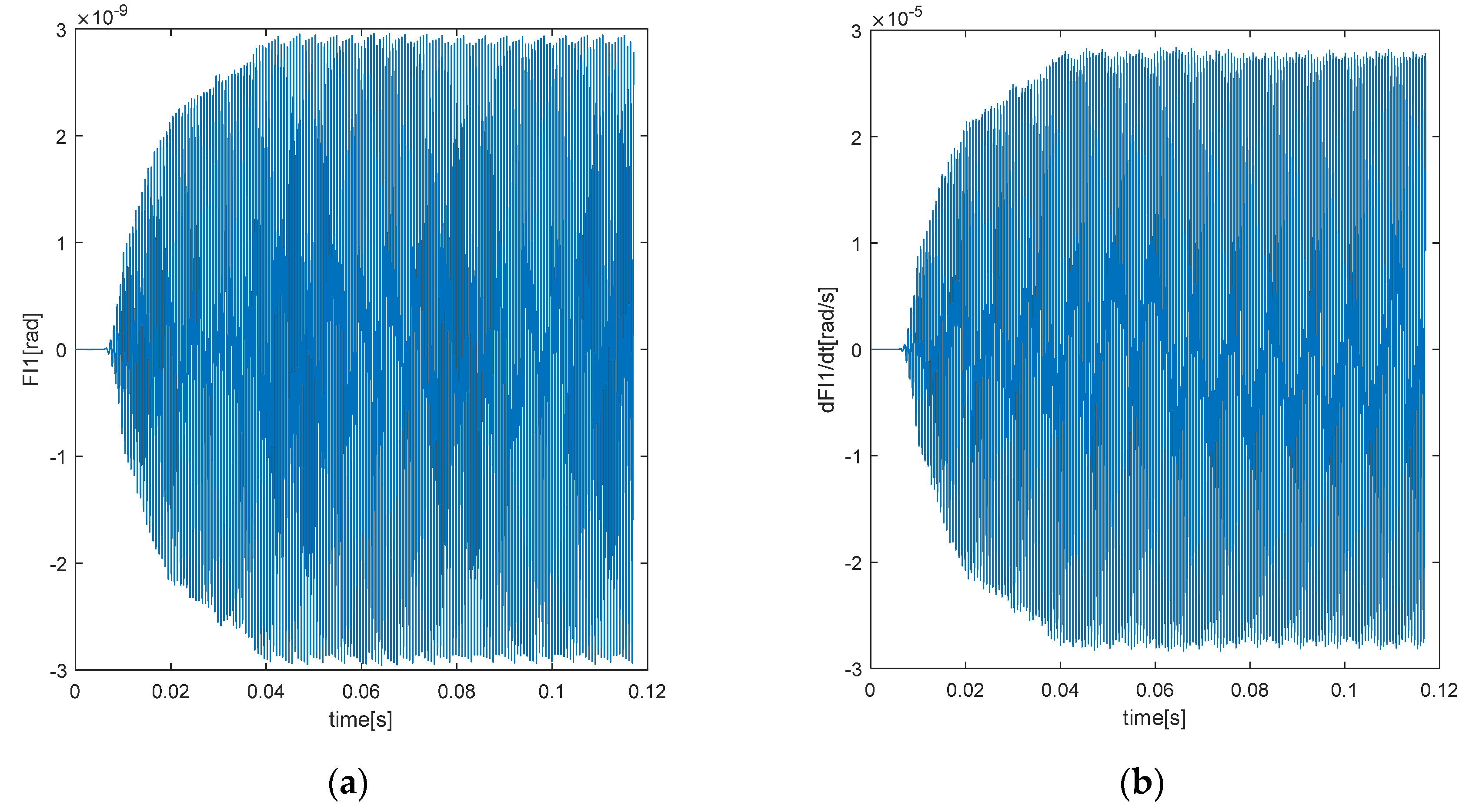
Figure 11, Figure 12 and Figure 13 illustrate the graphs of time–history to analyze the dynamic instability of NFTV for DTID’s DIE1 in transition through PPRR ${\mathsf{\eta }}_1\simeq 3066\hspace{0.17em}\mathrm{H}\mathrm{z}$ (see Equation (27), Figure 9, and Table 1), considering the worst misalignment for DIE1 ${\mathsf{\beta }}_1=9^0$, ${\mathsf{\Omega }}_1=9632\hspace{0.17em}\mathrm{r}\mathrm{a}\mathrm{d}/\mathrm{s}$ (see Equation (22), Table 1), ${\chi }_{\mathrm{n}\mathrm{D}\mathrm{I}\mathrm{E}1}=0.0026$, and the damping ratio $\mathsf{\xi }=0.0016\dots 0.0129$. MATLAB software was developed based on Equation (25) for NFTV of DIE1 to calculate the time–history $\left({\mathsf{\phi }}_1(\mathrm{t}),\mathrm{t}\right),(\frac{\mathrm{d}{\mathsf{\phi }}_1}{\mathrm{d}\mathrm{t}}(\mathrm{t}),\mathrm{t}),\left({\mathsf{\phi }}_1(\mathrm{t}),\frac{\mathrm{d}{\mathsf{\phi }}_1}{\mathrm{d}\mathrm{t}}(\mathrm{t}),\mathrm{t}\right),\left({\mathsf{\phi }}_1(\mathrm{t}),\frac{\mathrm{d}{\mathsf{\phi }}_1}{\mathrm{d}\mathrm{t}}(\mathrm{t})\right)$.

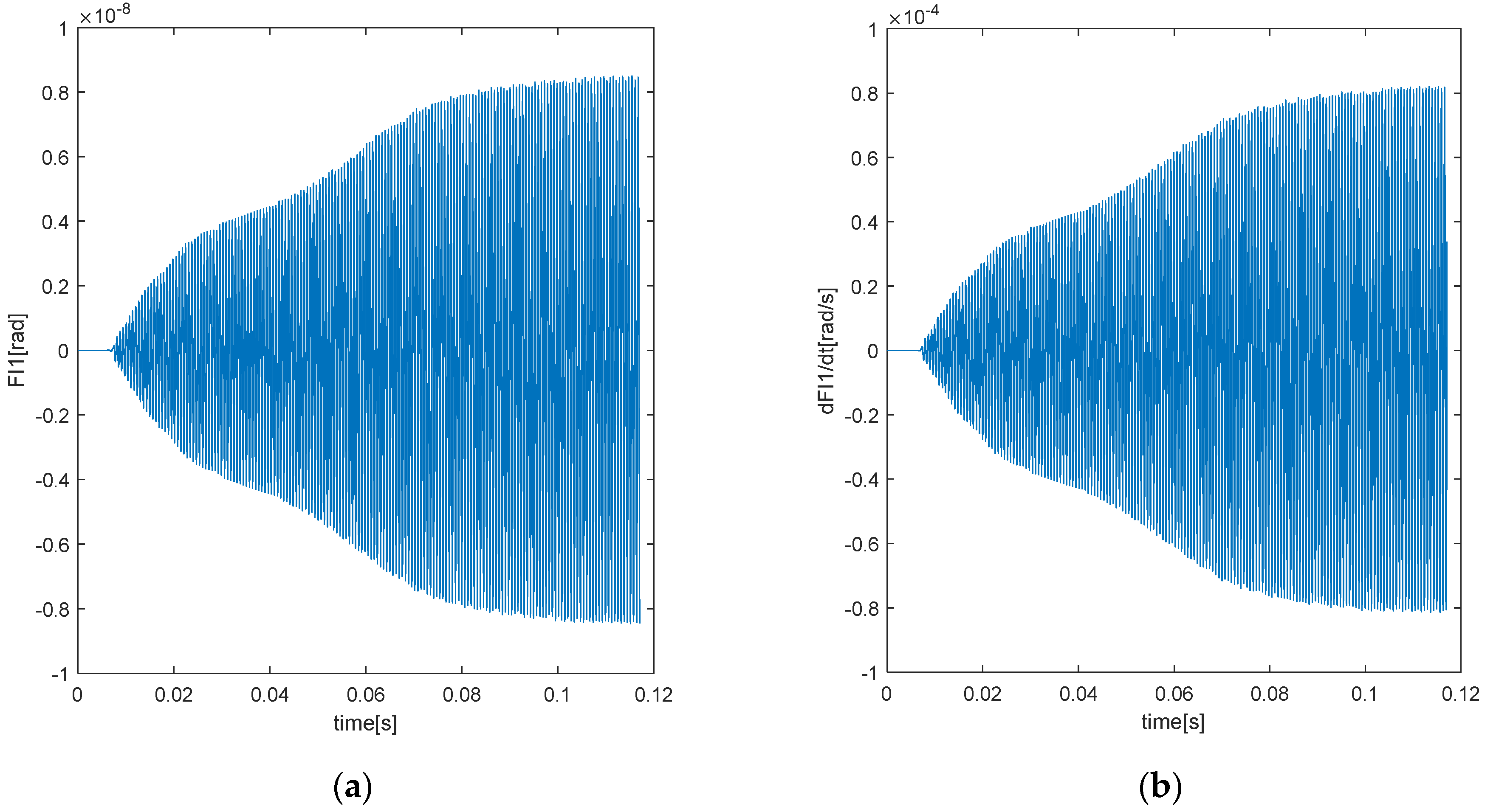
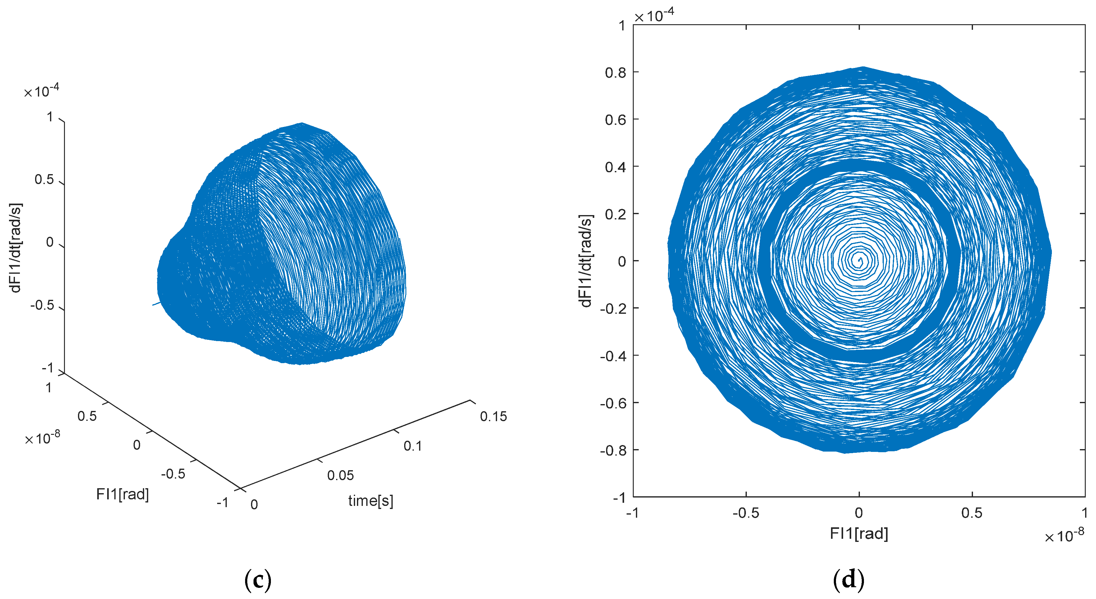
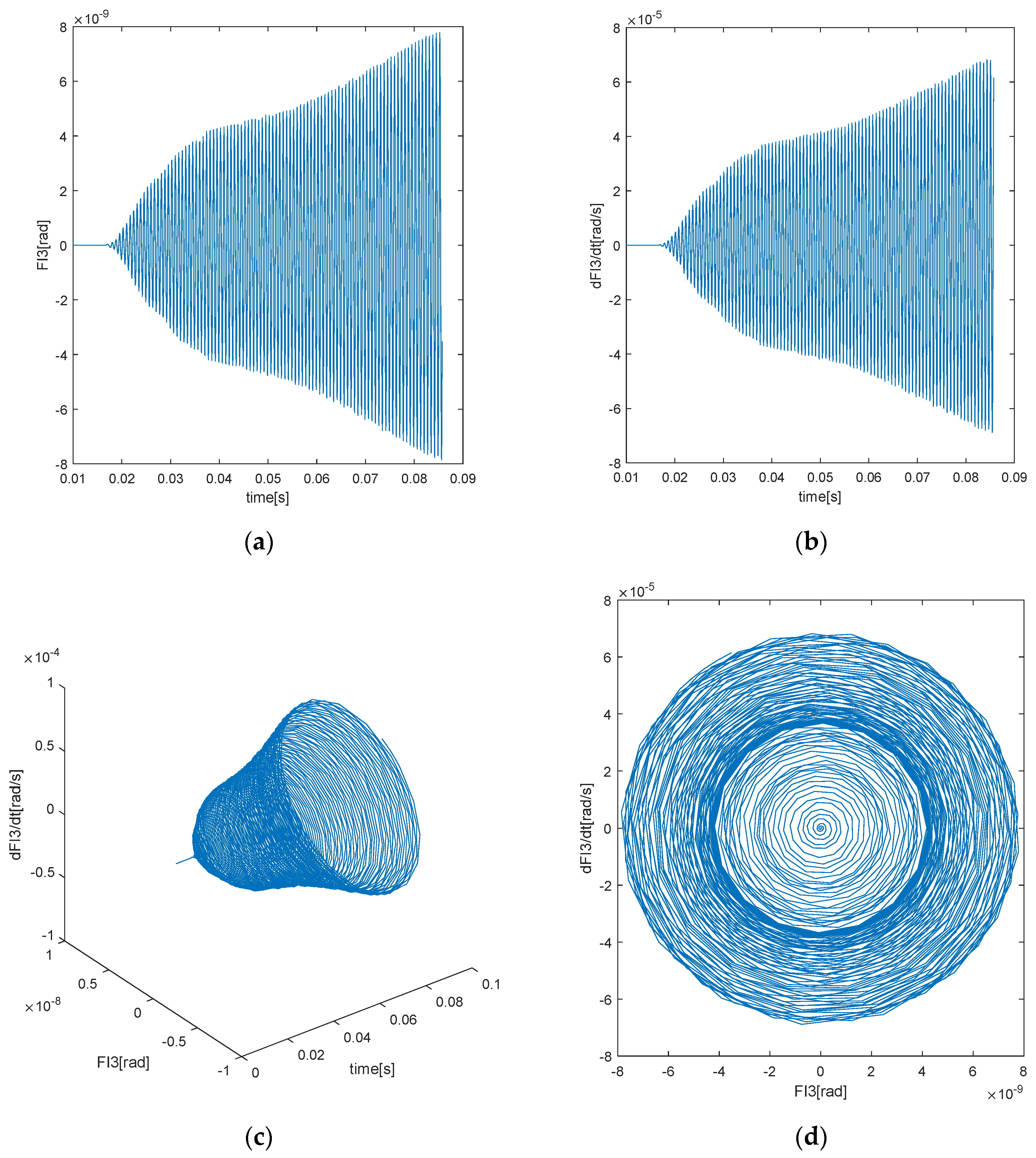
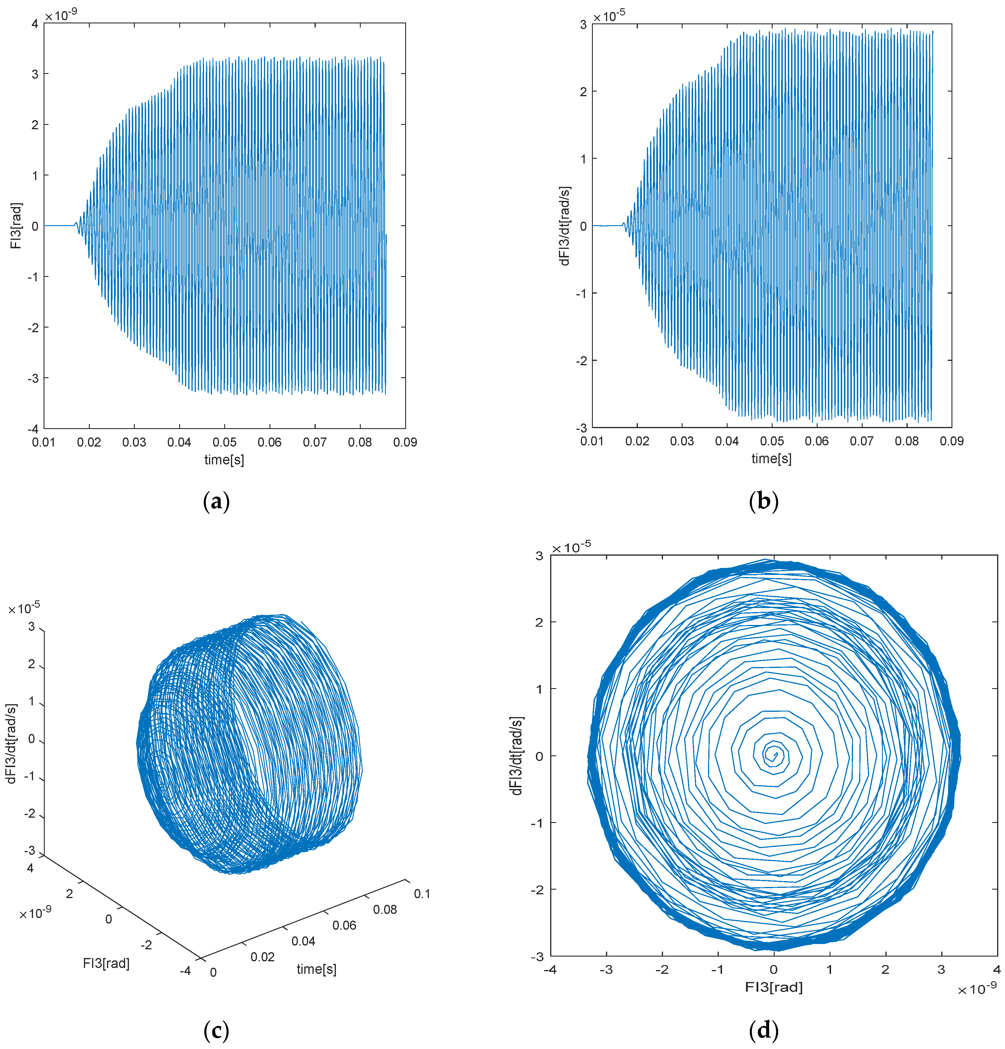
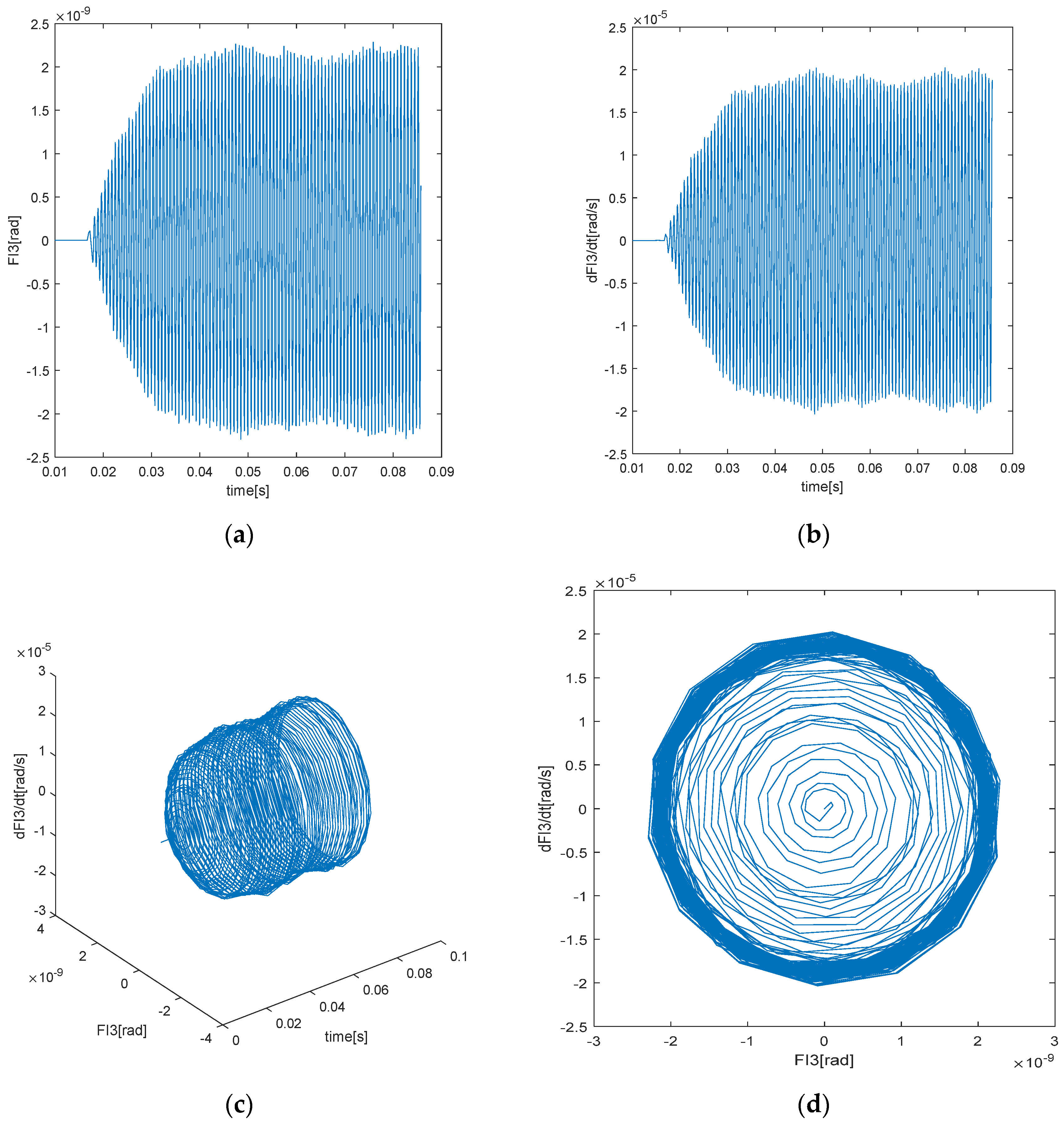
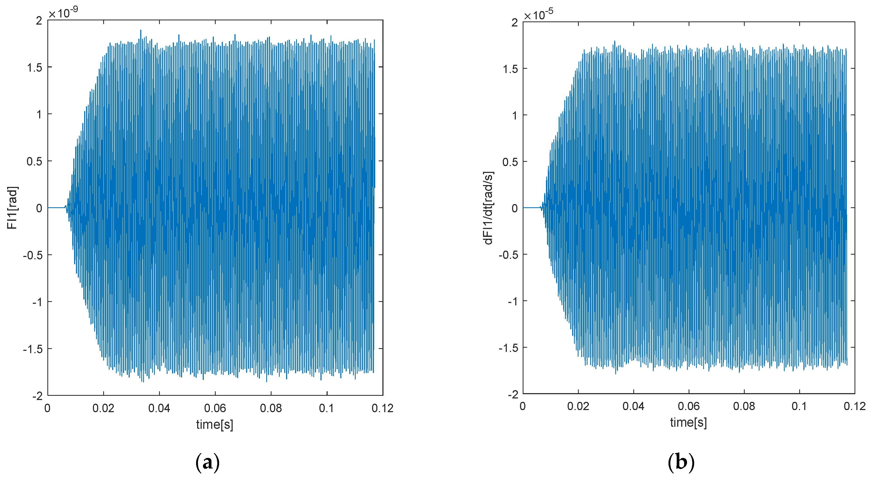
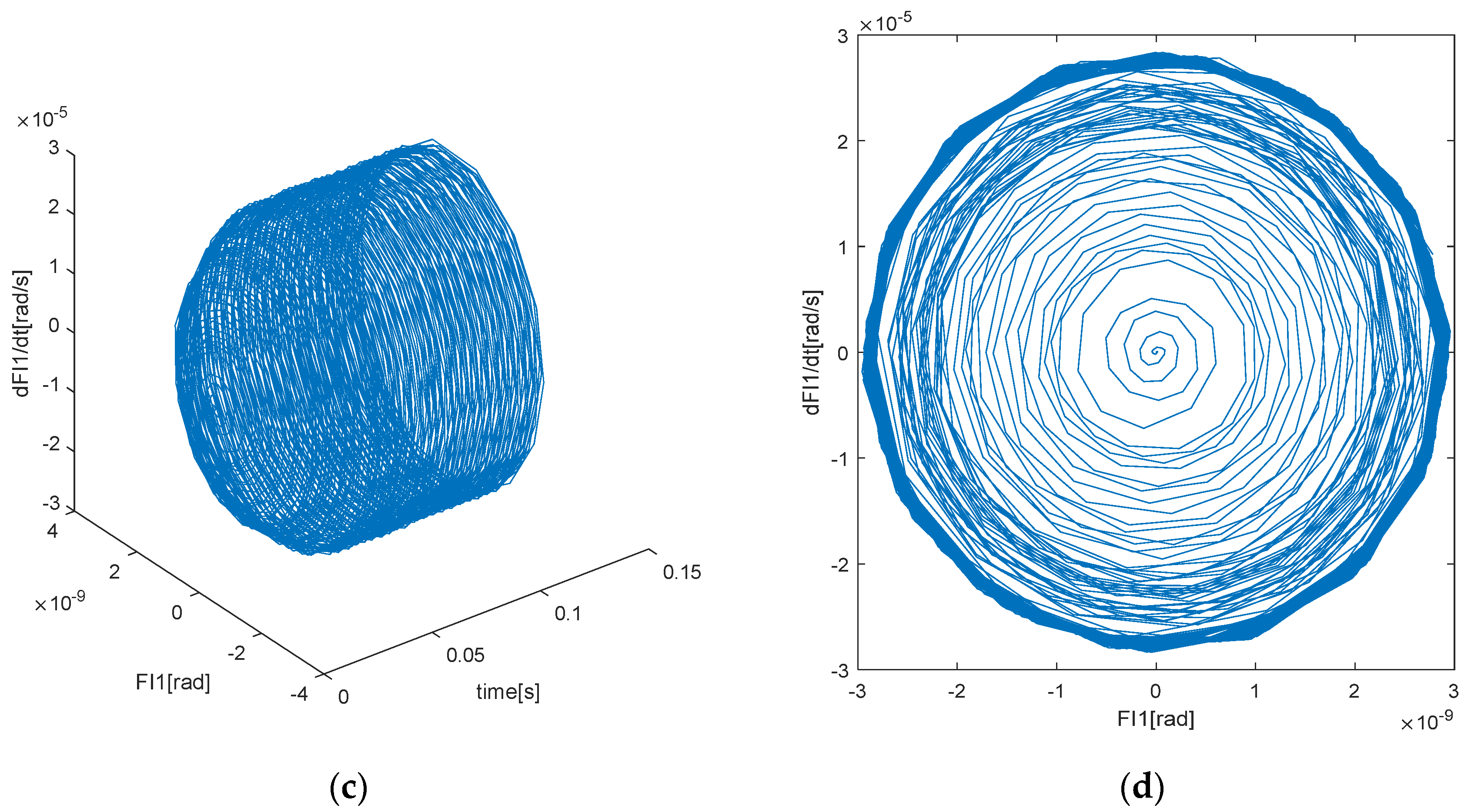
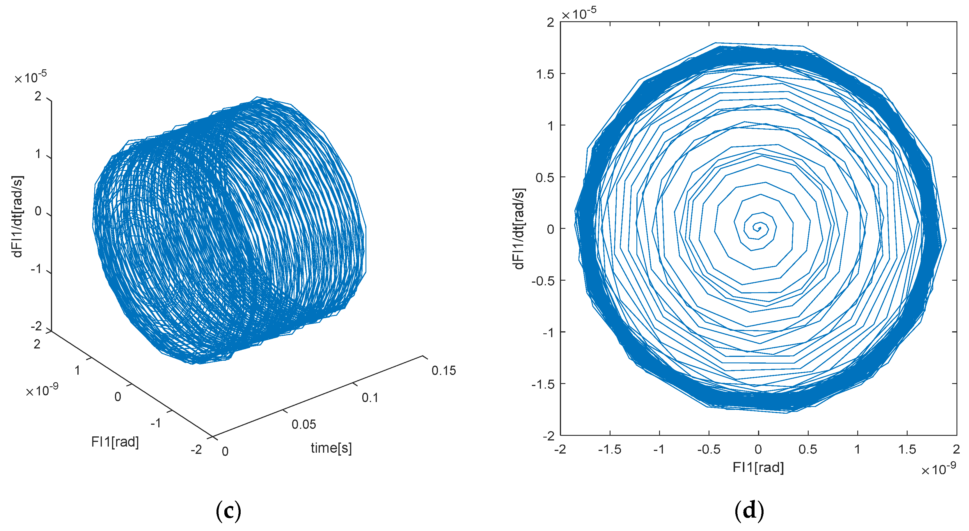
In Figure 11a–c, Figure 12a–c and Figure 13a–c, it is remarked that the nonstationary ${\mathsf{\phi }}_1(\mathrm{t})$, $\frac{\mathrm{d}{\mathsf{\phi }}_1}{\mathrm{d}\mathrm{t}}(\mathrm{t})$ for NFTV of DIE1 manifests the “beatings” effects and a rapid decrease of the extreme values with the damping’s increases in the range $(1.6\dots 12.9){10}^{-3}$. Figure 11d, Figure 12d and Figure 13d illustrate that the phase portraits represent the chaotic manifestation of a strange attractor for $\mathsf{\xi }=1.6\cdot {10}^{-3}$ and $\mathsf{\xi }=7.3\cdot {10}^{-3}$, multiple limit cycles and “turning points”, respectively, while for $\mathsf{\xi }=12.9\cdot {10}^{-3}$ only a limit cycle is manifested meaning that the nonstationary dynamic behavior for DIE1 has an ergodic manifestation starting from the value of the damping ratio.

The results obtained in Figure 11d, Figure 12d and Figure 13d show the similarity of the phase portrait pictures when compared with data in the literature [33]. It is noted that “pictures” in Figure 11d and Figure 12d are like those specific to a strange attractor. In this way, the aim of using time–history analysis (THA) for NFTV of DIE1 was reached, THA being thus a detection method for chaos manifestation of NFTV for the elements of DTID. For the cases when the damping ratio is in the vicinity range $\mathsf{\xi }=(1.6\dots 7.3)\cdot {10}^{-3}$, the deterministic chaos of NFTV for DIE1 needs to be certified using the new robust method LEA–PM.

Figure 14, Figure 15 and Figure 16 illustrate the graphs of time–history to analyze the dynamic instability of NFTV for DTID’s DOE3 in transition through PPRR ${\mathsf{\eta }}_3\simeq 2792\hspace{0.17em}\mathrm{H}\mathrm{z}$ (see Equation (28), Figure 10, and Table 2), considering the worst misalignment for DOE3 ${\mathsf{\beta }}_2=9^0,$ ${\mathsf{\Omega }}_3=8767\hspace{0.17em}\mathrm{r}\mathrm{a}\mathrm{d}/\mathrm{s}$ (see Equation (23) and Table 2), ${\chi }_{\mathrm{n}\mathrm{D}\mathrm{O}\mathrm{E}3}=0.0027,$ and the damping ratio $\mathsf{\xi }=0.0016\dots 0.0112$. MATLAB software was developed based on Equation (26) for NFTV of DOE3 to calculate the time–history $\left({\mathsf{\phi }}_3(\mathrm{t}),\mathrm{t}\right),(\frac{\mathrm{d}{\mathsf{\phi }}_3}{\mathrm{d}\mathrm{t}}(\mathrm{t}),\mathrm{t}),\left({\mathsf{\phi }}_3(\mathrm{t}),\frac{\mathrm{d}{\mathsf{\phi }}_3}{\mathrm{d}\mathrm{t}}(\mathrm{t}),\mathrm{t}\right),\left({\mathsf{\phi }}_3(\mathrm{t}),\frac{\mathrm{d}{\mathsf{\phi }}_3}{\mathrm{d}\mathrm{t}}(\mathrm{t})\right)$.

In Figure 14a–c, Figure 15a–c and Figure 16a–c, it is remarked that the nonstationary ${\mathsf{\phi }}_3(\mathrm{t})$, $\frac{\mathrm{d}{\mathsf{\phi }}_3}{\mathrm{d}\mathrm{t}}(\mathrm{t})$ for NFTV of DOE3 manifests the same “beatings” effects and a rapid decrease of the extreme values with the damping’s increases in the range $(1.6\dots 11.2){10}^{-3}$ as for DIE1 (see Figure 11a–c, Figure 12a–c and Figure 13a–c). The graphs illustrated in Figure 14d, Figure 15d and Figure 16d show that the phase portraits represent the chaotic manifestation of a strange attractor for $\mathsf{\xi }=1.6\cdot {10}^{-3}$ and $\mathsf{\xi }=6.4\cdot {10}^{-3}$, multiple limit cycles and “turning points”, respectively, while for $\mathsf{\xi }=11.2\cdot {10}^{-3}$ only a limit cycle is manifested meaning that the nonstationary dynamic behavior for DOE3 has an ergodic manifestation starting from this value of the damping ratio.

The similarity of the phase portrait pictures is shown when comparing the results obtained in Figure 14d, Figure 15d and Figure 16d with data in the literature [33]. It is noted that “pictures” in Figure 14d and Figure 15d are like those specific to a strange attractor. In this way, the aim of using THA for NFTV of DOE3 was reached, THA being thus a detection method for chaos manifestation of NFTV for the elements of DTID. For the cases when the damping ratio is in the vicinity range $\mathsf{\xi }=(1.6\dots 7.3)\cdot {10}^{-3}$ the deterministic chaos of NFTV for DIE1 needs to be certified using the new robust method LEA–PM.

As can be seen from Figure 11, Figure 12, Figure 13, Figure 14, Figure 15 and Figure 16, the THA (phases portraits, all the d. figures) was used as a detection method for possible chaotic dynamic manifestations of the DTID’s elements (DIE1 and DOE3). Amer et al. [34], had used time–history analysis to study the steady-state nonlinear motion of a damped spring pendulum with an attached linear damped transverse absorber near resonance (primary external and internal resonance) and to investigate the stability of fixed points. Based on this kind of investigation, the above-mentioned dynamic system found that the motion is free of chaos motion [34] (p. 32). Liu et al. [35] use the THA to investigate the stability of nonlinear behavior of a spur gear pair transmission system with backlash, finding the trends in the unstable conditions of these systems. Azimi [36], after employing the Pitchfork and Hops Bifurcations to investigate the geared systems in permanent contact, used THA coupled with the Poincaré Map Method to detect the creation of limit cycles (new equilibria) in the case of nonlinear softening behavior of geared systems transmission. Zhang et al. [37] investigated the mechanism and the characteristics of the varying global compliance (VC) parametric resonances in ball bearings using time–history analysis, phases orbits analysis, Poincaré Map Method, and frequency spectra. Thus, the chaotic motions were detected and certified. Rysak and Gregorczyk [38], calibrated the order of integration of the differential transform method (DTM) using THA for the fractional chaotic Rössler system.

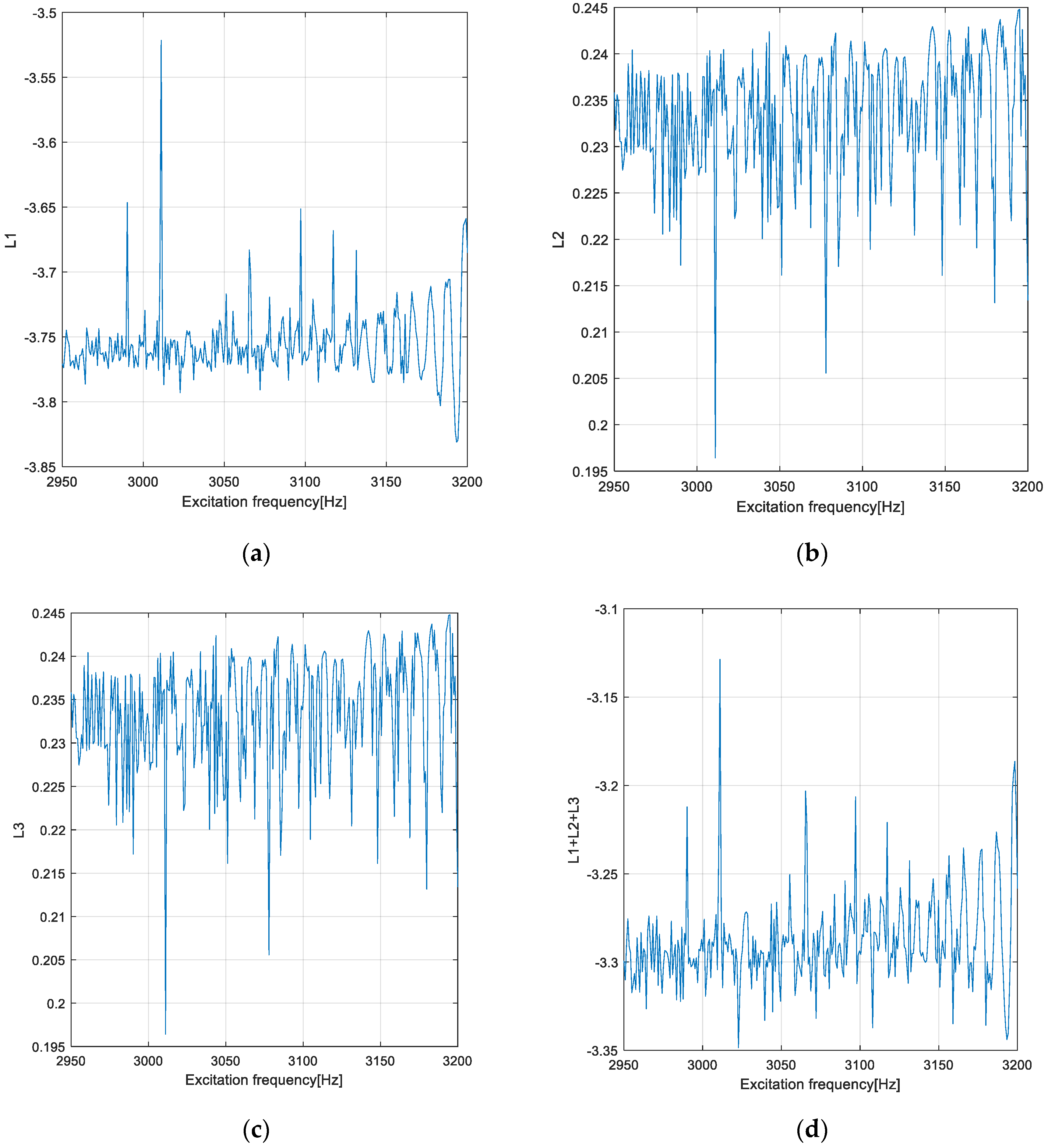
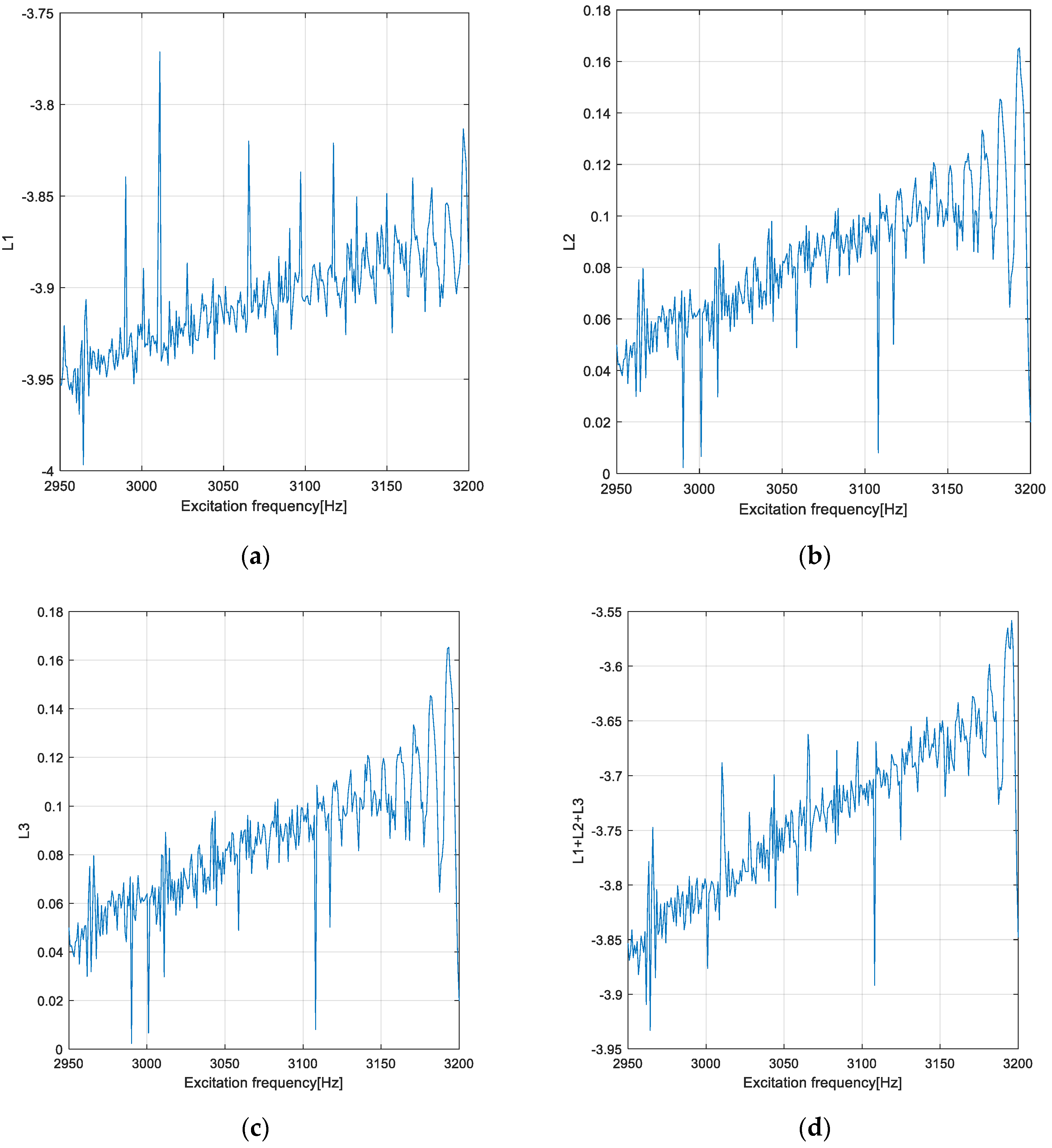
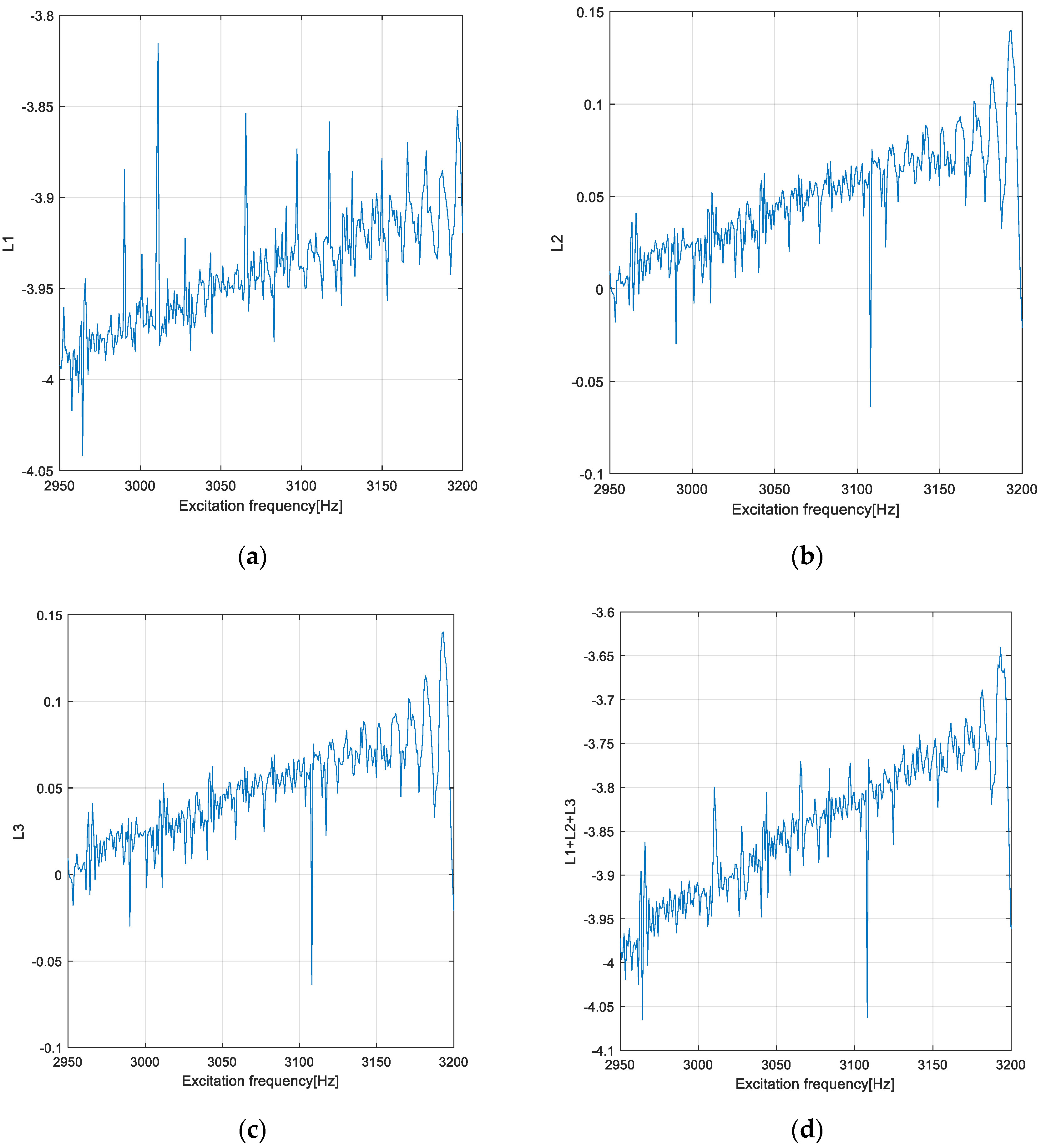
The new method presented in paragraph 5 uses LEA–PM to certify the deterministic chaos. Based on Equations (31)–(33), developing specific MATLAB software, the Lyapunov exponents for the DSOE (29) of NFTV were computed for DIE1 in transition through PPRR. The results are illustrated in Figure 17, Figure 18, Figure 19 and Figure 20 for the characteristic values of DIE1, such as excitation frequency in the vicinity of ${\mathsf{\eta }}_1=3066$ Hz (see Equation (27), Figure 9, and Table 1), ${\mathsf{\beta }}_1=9^0$, ${\mathsf{\Omega }}_1=9632\hspace{0.17em}\mathrm{r}\mathrm{a}\mathrm{d}/\mathrm{s}$ (see Equation (22), Table 1), ${\chi }_{\mathrm{n}\mathrm{D}\mathrm{I}\mathrm{E}1}=0.0026$, and the damping ratio in the range $\mathsf{\xi }=0.0016\dots 0.0114$.

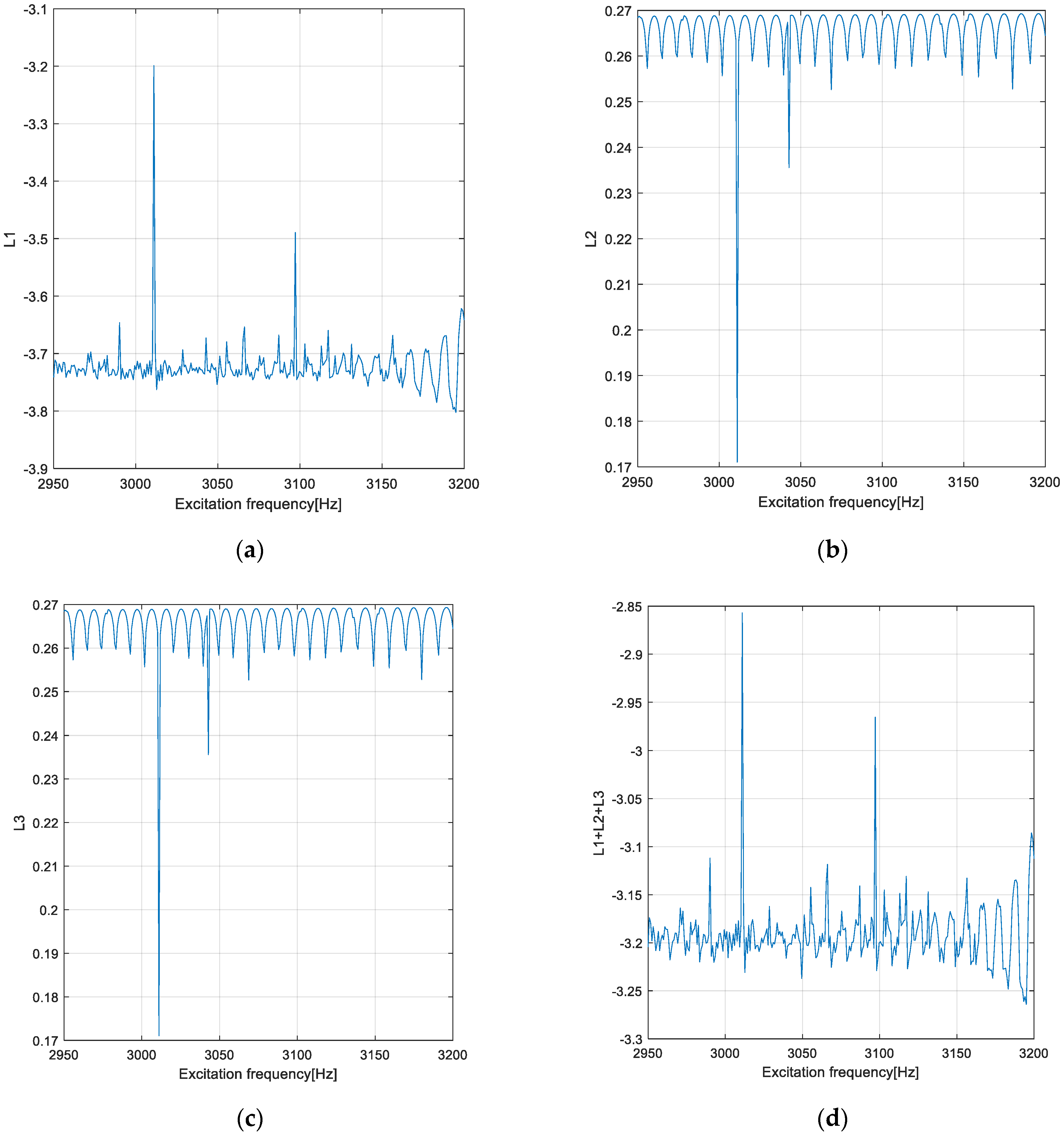
As can be seen from the Figure 17, Figure 18, Figure 19 and Figure 20 in (a) is presented the graph variation of the Lyapunov exponent ${\mathrm{L}}_{11}$ (see Equation (31), to verify the criteria (37)), in (b) is illustrated the graph variation of the Lyapunov exponent ${\mathrm{L}}_{21}$ ( see Equation (32), to verify the criteria (37)), in (c) is shown the graph variation of the Lyapunov exponent ${\mathrm{L}}_{31}$ ( see Equation (33), to verify the criteria (37)), and in (d) is presented the graph variation of the sum of Lyapunov exponents ${\mathrm{L}}_{11}+{\mathrm{L}}_{21}+{\mathrm{L}}_{31}$ (in order to apply the criteria (39)), for the nonstationary FTV of DIE1 in transition through the PPRR, namely for excitation frequency in the range [2950,3200] Hz.

Through the analysis of the graphs illustrated in Figure 17, it can be concluded that the conditions imposed by Equations (37)–(39), as mentioned in [23,31], are fulfilled and, therefore, in the excitation frequency’s range of 2950–3200 Hz, the range of PPRR for FTV of DIE1, for $\mathsf{\xi }=1.6\cdot {10}^{-3}$ the deterministic chaos (strange attractor) is manifested. For certification of this manifestation, the last part of the new robust method LEA–PM, the qualitative PMM, will be used.

Through the analysis of the graphs illustrated in Figure 18, it can be concluded that the conditions imposed by Equations (37)–(39), as mentioned in [23,31], are fulfilled and, therefore, in the excitation frequency’s range of 2950–3200 Hz, the range of PPRR for FTV of DIE1, for $\mathsf{\xi }=7.3\cdot {10}^{-3}$ the deterministic chaos (strange attractor) is manifested. For certification of this manifestation, the last part of the new robust method LEA–PM, the qualitative PMM, will be used.

Through the analysis of the graphs illustrated in Figure 19, it can be concluded that the conditions imposed by Equations (37)–(39), as mentioned in [23,31], are fulfilled and, therefore, in the excitation frequency’s range of 2950–3200 Hz, the range of PPRR for FTV of DIE1, for $\mathsf{\xi }=11\cdot {10}^{-3}$ the deterministic chaos (strange attractor) is manifested. For certification of this manifestation, the last part of the new robust method LEA–PM, the qualitative PMM, will be used.

Through the analysis of the graphs illustrated in Figure 20, it can be concluded that the conditions imposed by Equations (37)–(39), as mentioned in [23,31], are not fulfilled and, therefore, in the excitation frequency’s range of 2950–3105 Hz, the range of PPRR for FTV of DIE1, for $\mathsf{\xi }=11.4\cdot {10}^{-3}$ the deterministic chaos (strange attractor) is not possible. Using LEA–PM, it is certified by the conditions imposed (37)–(39) that for damping ratio in the range $\mathsf{\xi }=(11.4\dots 18.6)\cdot {10}^{-3}$ the NFTV of DIE1 in transition through PPRR is an ergodic dynamic behavior representing a transition to chaos, as mentioned in [23].

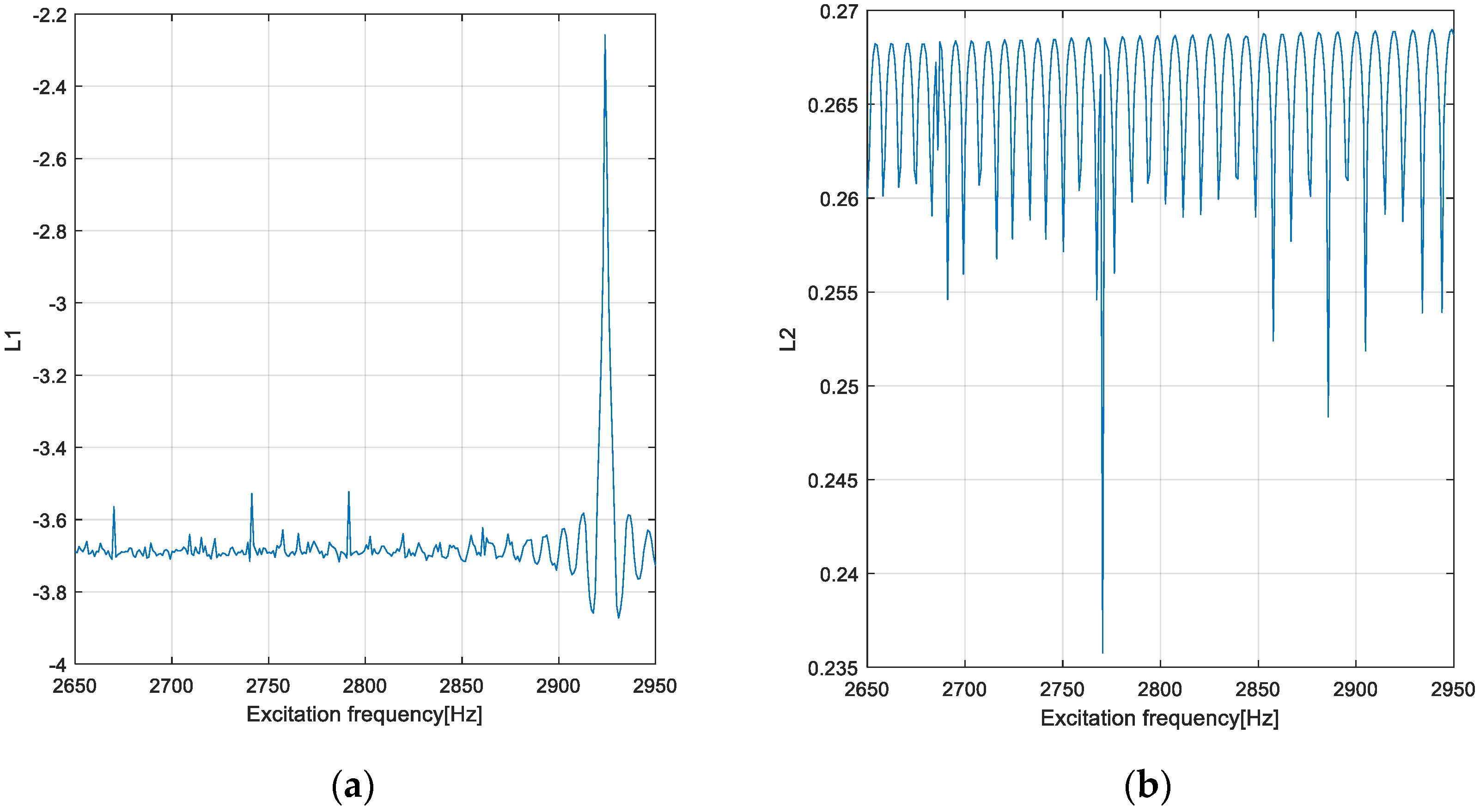
Based on Equations (34)–(36), developing specific MATLAB software, the Lyapunov exponents for the DSOE (30) of NFTV were computed for DOE3 in transition through PPRR. The results are illustrated in Figure 21, Figure 22, Figure 23 and Figure 24 for the characteristic values of DOE3, such as excitation frequency in the vicinity of ${\mathsf{\eta }}_3\simeq 2792\hspace{0.17em}\mathrm{H}\mathrm{z}$ (see Equation (28), Figure 10, and Table 2), ${\mathsf{\beta }}_2=9^0$, ${\mathsf{\Omega }}_3=8767\hspace{0.17em}\mathrm{r}\mathrm{a}\mathrm{d}/\mathrm{s}$ (see Equation (23) and Table 2), ${\chi }_{\mathrm{n}\mathrm{D}\mathrm{O}\mathrm{E}3}=0.0027$, and the damping ratio in the range $\mathsf{\xi }=0.0016\dots 0.0114$.

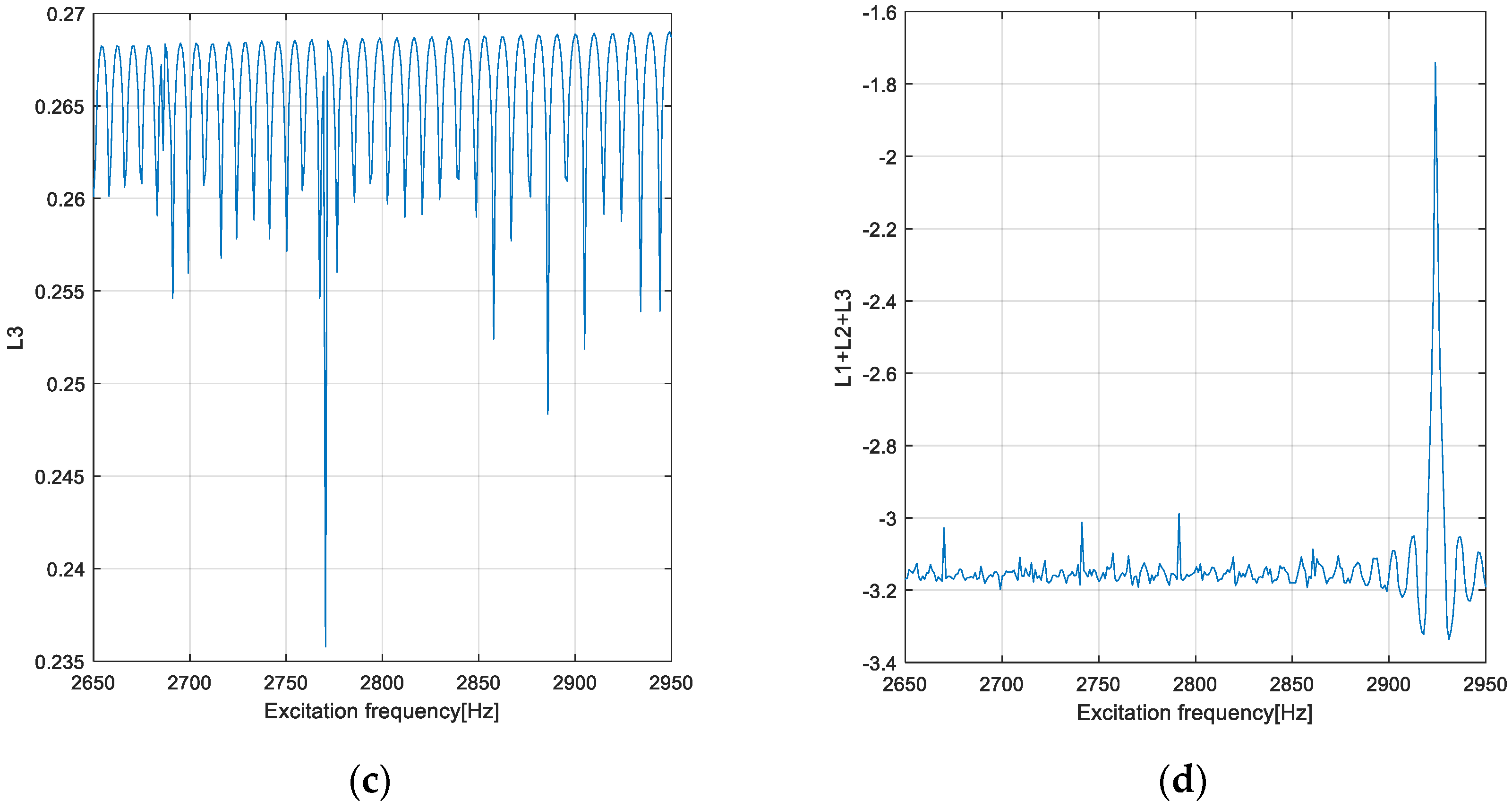
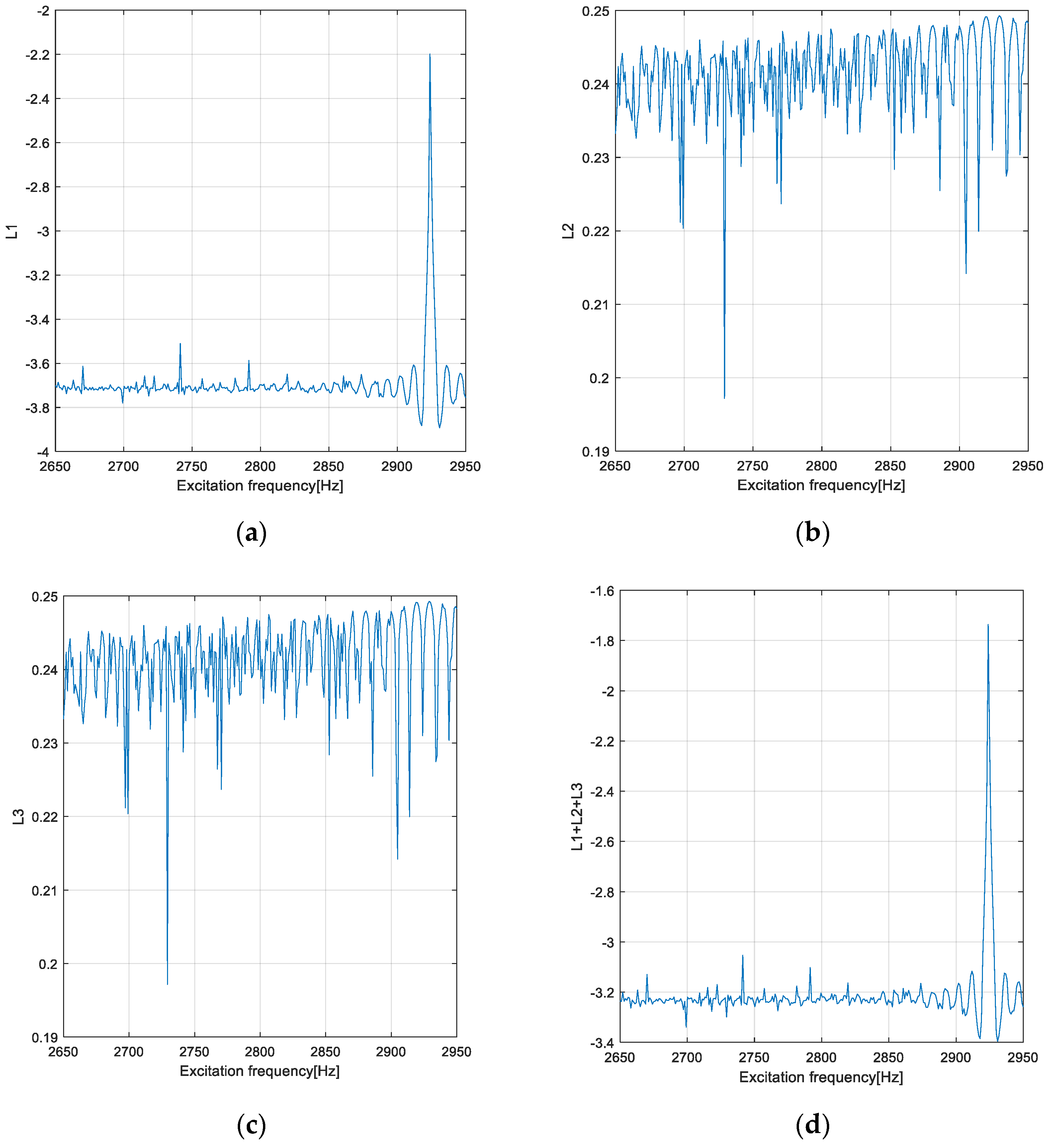
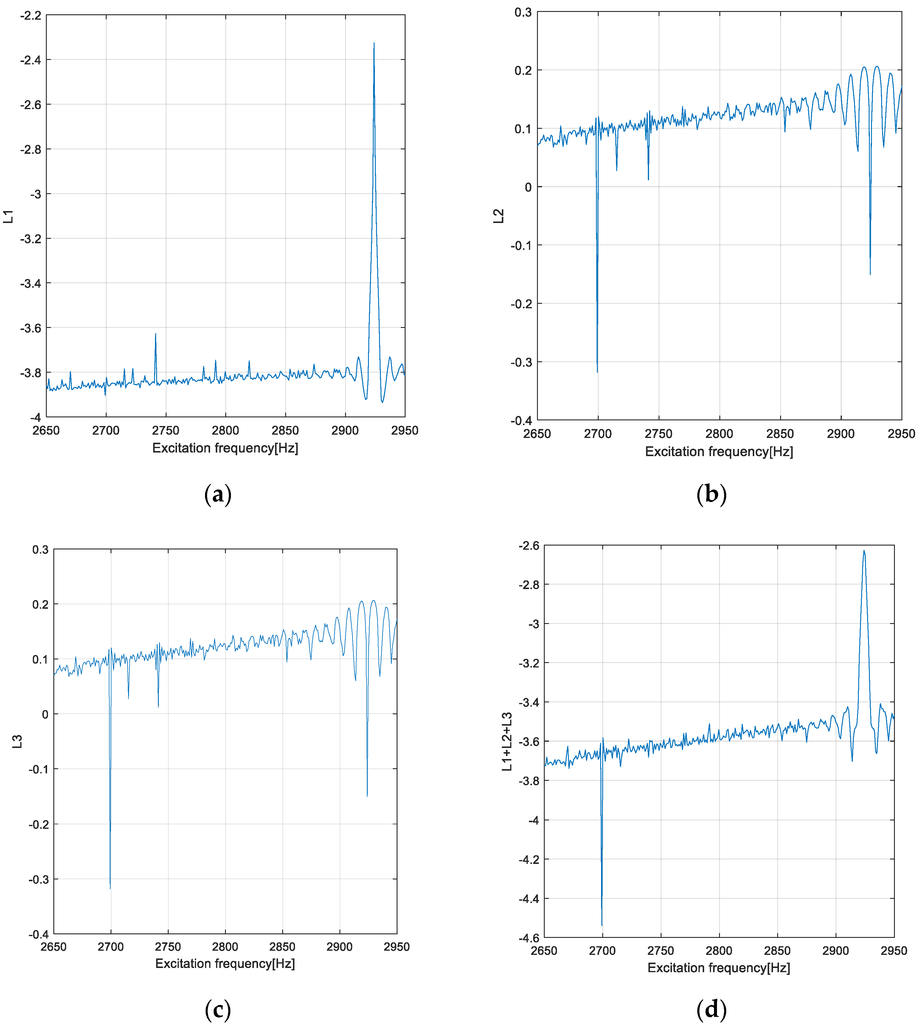
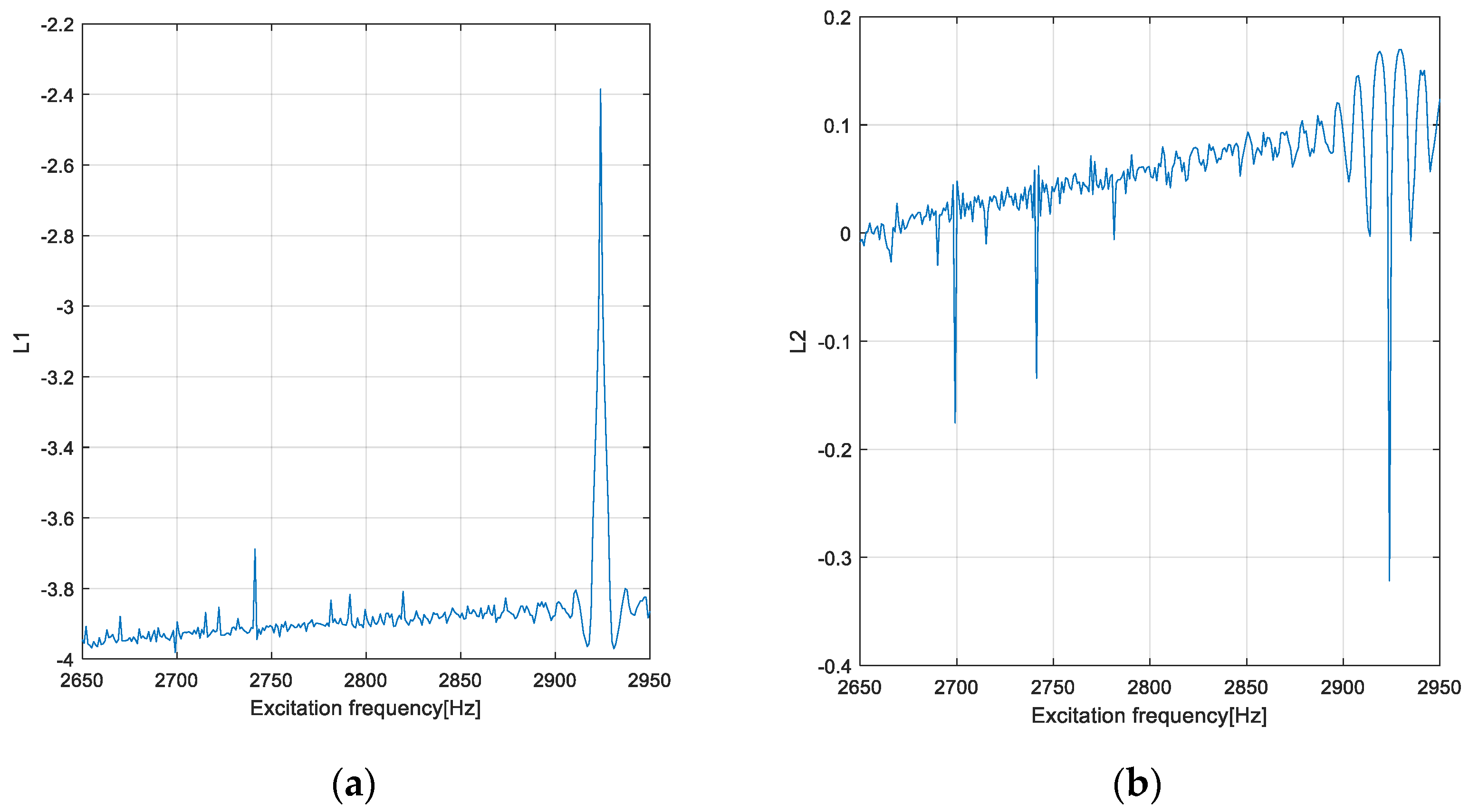
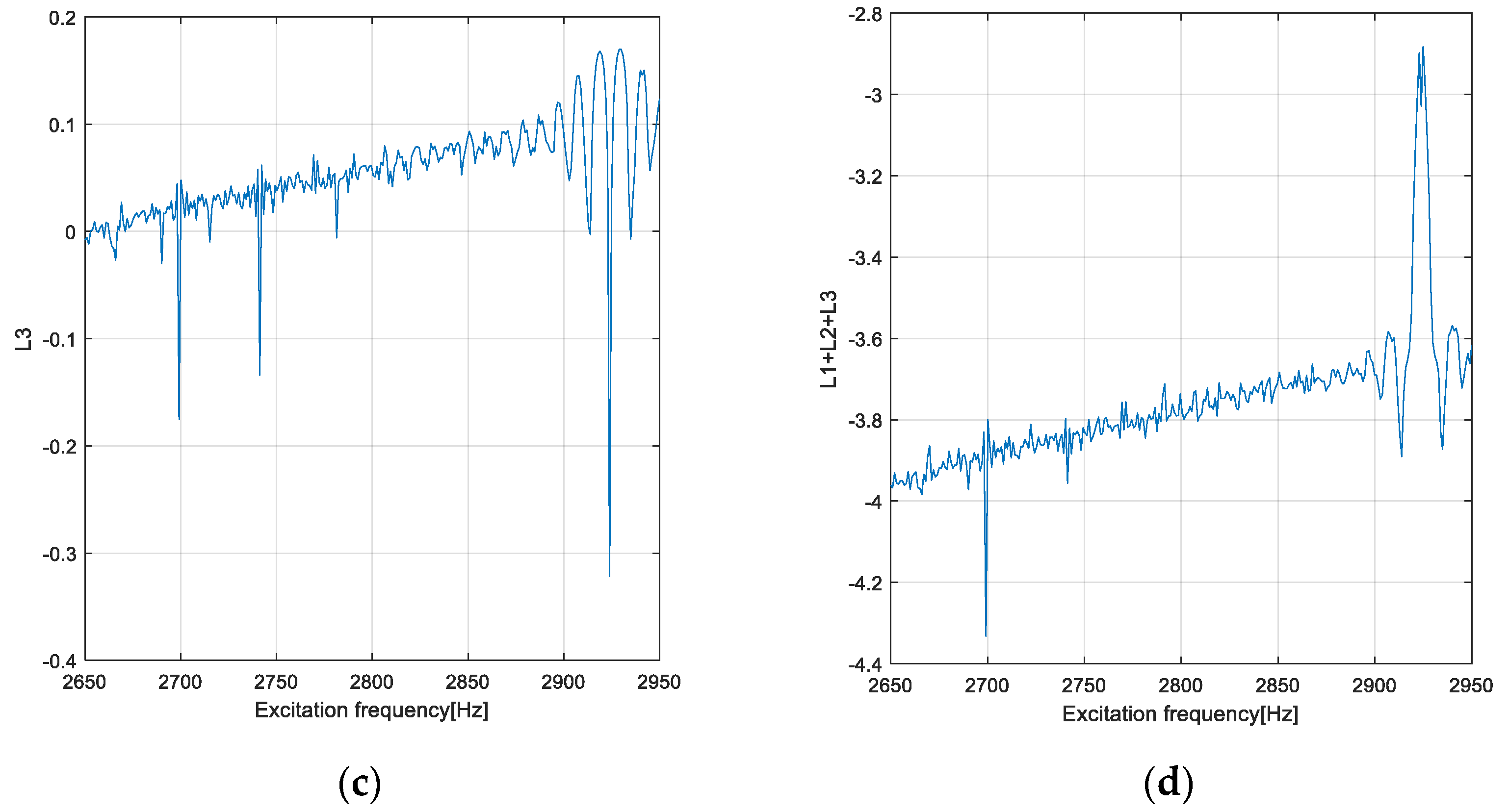
As can be seen from the Figure 21, Figure 22, Figure 23 and Figure 24 in (a) is presented the graph variation of the Lyapunov exponent ${\mathrm{L}}_{13}$ (see Equation (34), to verify the criteria (37)), in (b) is illustrated the graph variation of the Lyapunov exponent ${\mathrm{L}}_{23}$ ( see Equation (35), to verify the criteria (37)), in (c) is shown the graph variation of the Lyapunov exponent ${\mathrm{L}}_{33}$ ( see Equation (36), to verify the criteria (37)), and in (d) is presented the graph variation of the sum of Lyapunov exponents ${\mathrm{L}}_{13}+{\mathrm{L}}_{23}+{\mathrm{L}}_{33}$ (in order to apply the criteria (39)), for the nonstationary FTV of DOE3 in transition through the PPRR, namely for excitation frequency in the range [2650,2950] Hz.

Through the analysis of the graphs illustrated in Figure 21, it can be concluded that the conditions imposed by Equations (37)–(39), as mentioned in [23,31], are fulfilled and, therefore, in the excitation frequency’s range of 2650–2950 Hz, the range of PPRR for FTV of DOE3, for $\mathsf{\xi }=1.6\cdot {10}^{-3}$ the deterministic chaos (strange attractor) is manifested. For certification of this manifestation, the last part of the new robust method LEA–PM, the qualitative PMM, will be used.

Through the analysis of the graphs illustrated in Figure 22, it can be concluded that the conditions imposed by Equations (37)–(39), as mentioned in [23,31], are fulfilled and, therefore, in the excitation frequency’s range of 2650–2950 Hz, the range of PPRR for FTV of DOE3, for $\mathsf{\xi }=6.4\cdot {10}^{-3}$ the deterministic chaos (strange attractor) is manifested. For certification of this manifestation, the last part of the new robust method LEA–PM respectively, the qualitative PMM, will be used.

Through the analysis of the graphs illustrated in Figure 23, it can be concluded that the conditions imposed by Equations (37)–(39), as mentioned in [23,31], are fulfilled and, therefore, in the excitation frequency’s range of 2700–2925 Hz, the range of PPRR for FTV of DOE3, for $\mathsf{\xi }=10.4\cdot {10}^{-3}$ the deterministic chaos (strange attractor) is manifested. For certification of this manifestation, the last part of the new robust method LEA–PM respectively, the qualitative PMM, will be used.

Through the analysis of the graphs illustrated in Figure 24, it can be concluded that the conditions imposed by Equations (37)–(39), as mentioned in [23,31], are not fulfilled and, therefore, in the excitation frequency’s range of 2670–2925 Hz, the range of PPRR for FTV of DOE3, for $\mathsf{\xi }=11.2\cdot {10}^{-3}$ the deterministic chaos (strange attractor) is not possible. Using LEA–PM, it is certified by the conditions imposed (37)–(39) that for damping ratio in the range $\mathsf{\xi }=(11.2\dots 16)\cdot {10}^{-3}$ the NFTV of DOE3 in transition through PPRR is an ergodic dynamic behavior representing a transition to chaos, as mentioned in [23]. Asokanthan and Meehan [39], investigated the nonlinear vibration of a basic torsional system driven by a Hooke’s joint using time–history analysis (THA) and the bifurcation analysis, and the quasi-periodic and chaotic motion were revealed. Asokanthan and Wang [40] studied the torsional instabilities in a Hooke’s joint-driven system via maximal Lyapunov’s exponents (the well-known MLEM). They found a direct link between the maximal Lyapunov exponents and the instability regions for subharmonic and combination resonances.

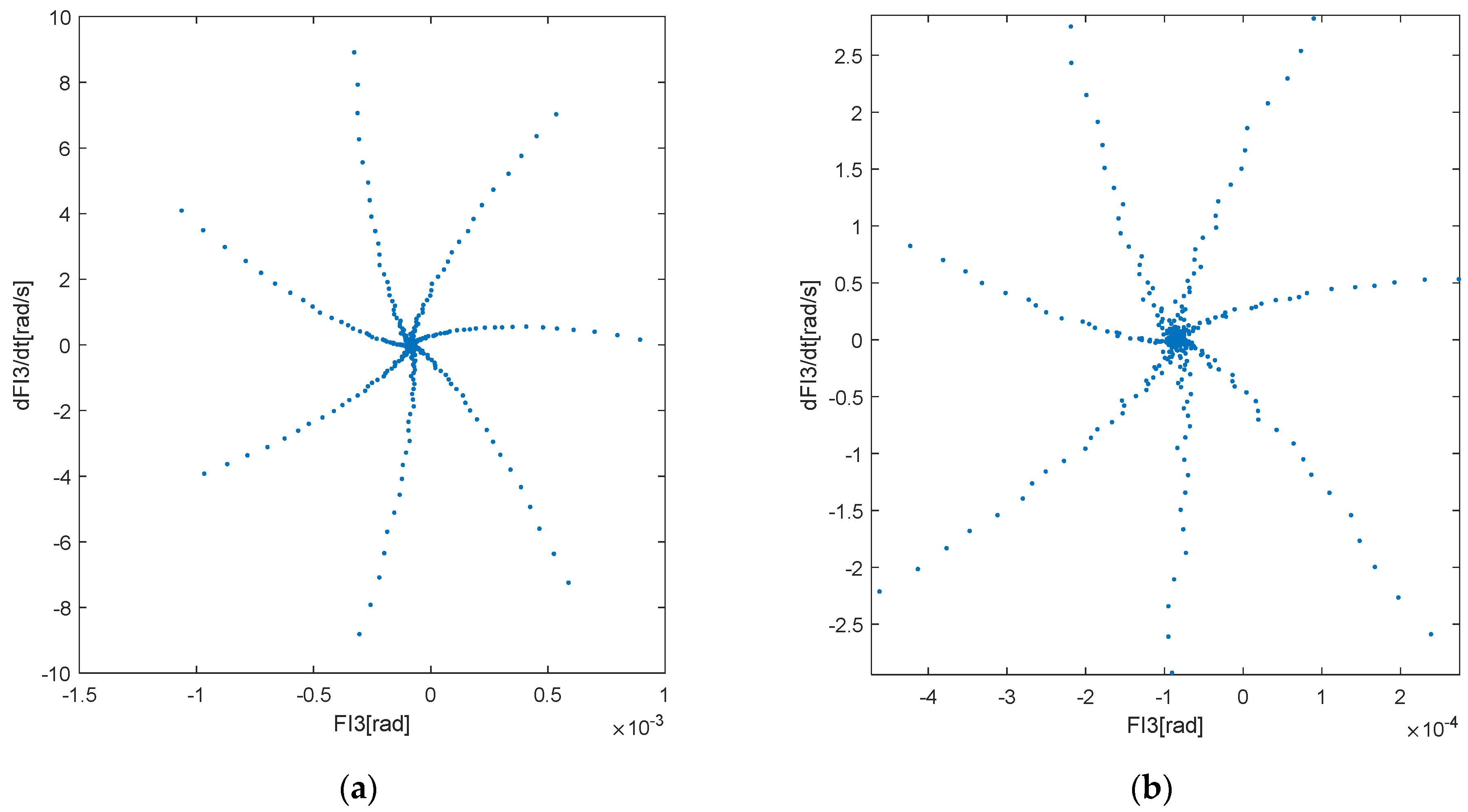
To certify using a qualitative method that the DIE1 and DOE3 have NFTV in the PPRR of chaotic type, MATLAB software was developed based on DSOE (29) for DIE1 and on DSOE (30) for DOE3, to represent the Poincaré Maps that represents the intersection of the orbits in the phase portraits with an orthogonal surface at equal periods (N number of points), using the mathematical procedure presented in [32] (p. 194). The Poincaré map represents saddle points or saddle separatrices images if the vibration motion is periodic or quasi-periodic. Figure 25 is presented the PM for DIE1 when $\mathsf{\xi }=1.6\cdot {10}^{-3}$, ${\mathsf{\eta }}_1=3066.5\hspace{0.17em}\mathrm{H}\mathrm{z}$ (see Equation (27), Figure 9, and Table 1), ${\mathsf{\beta }}_1=9^0$ using 50,000, 15,000, 10,000, and 1000 sections of orthogonal surface to the orbits in the phase portrait $\left({\mathsf{\phi }}_1,\frac{\mathrm{d}{\mathsf{\phi }}_1}{\mathrm{d}\mathrm{t}}\right).$

From the phase portraits illustrated in Figure 25, the properties of PM can be noted in the case of strange attractor: diffuse structure of points having a different density of pixels per unit area of the surface and auto-similarity of the image.

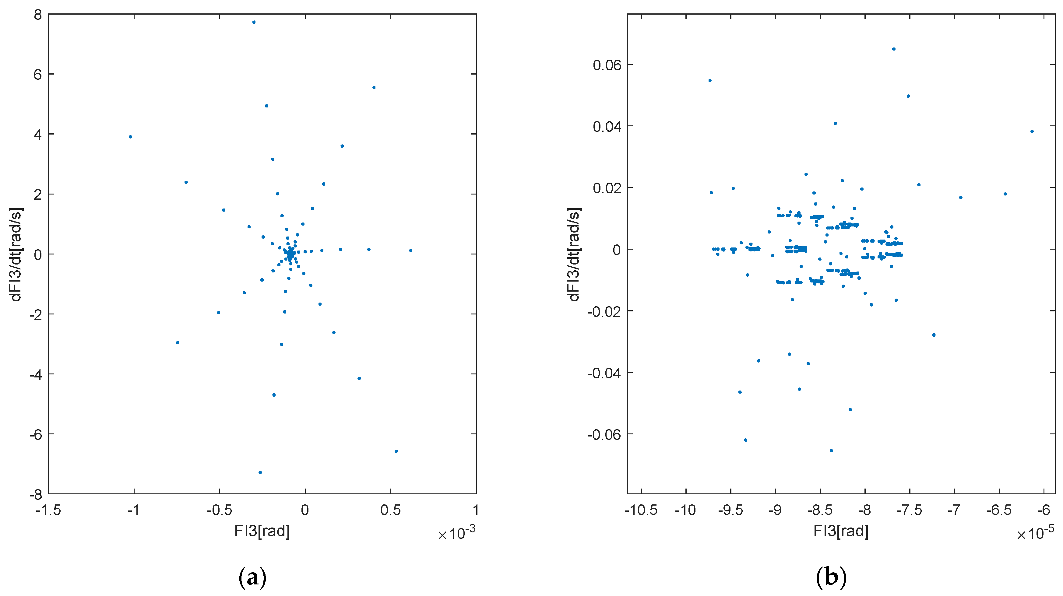
Figure 26 and Figure 27 present the PM for DIE1 when $\mathsf{\xi }=7.3\cdot {10}^{-3},{\mathsf{\eta }}_1=3066.5\hspace{0.17em}\mathrm{H}\mathrm{z},{\mathsf{\beta }}_1=9^0$ and $\mathsf{\xi }=11\cdot {10}^{-3},{\mathsf{\eta }}_1=3066.5\hspace{0.17em}\mathrm{H}\mathrm{z},{\mathsf{\beta }}_1=9^0$ using 15,000 to 1000 sections of orthogonal surface to the orbits in the phase portrait $\left({\mathsf{\phi }}_1,\frac{\mathrm{d}{\mathsf{\phi }}_1}{\mathrm{d}\mathrm{t}}\right).$ Images illustrated in Figure 26 have the aspects of a strange attractor.

The aspect of the image in Figure 26 has a chaotic manifestation specific to deterministic chaos (strange attractor), and the aspect of the images of both Figure 26 and Figure 27 are like those presented in Figure 25.

Comparing the images presented in Figure 26 with those illustrated in Figure 27, it can be concluded that the strange attractor started to vanish because we were close to the condition $\mathsf{\xi }=11.4\cdot {10}^{-3}$ when it is manifested in the ergodic dynamic process of DIE1 (see Figure 24). The pictures illustrated in Figure 25, Figure 26 and Figure 27 represent the final confirmation for the occurrence of deterministic chaos (strange attractor) (see Figure 17, Figure 18 and Figure 19) for the NFTV of DIE1 in PPRR for ${\mathsf{\beta }}_1=9^0,{\mathsf{\eta }}_1=3066.5\hspace{0.17em}\mathrm{H}\mathrm{z}$ and damping ratio in the range $\mathsf{\xi }=(1.6\dots 11)\cdot {10}^{-3}$.

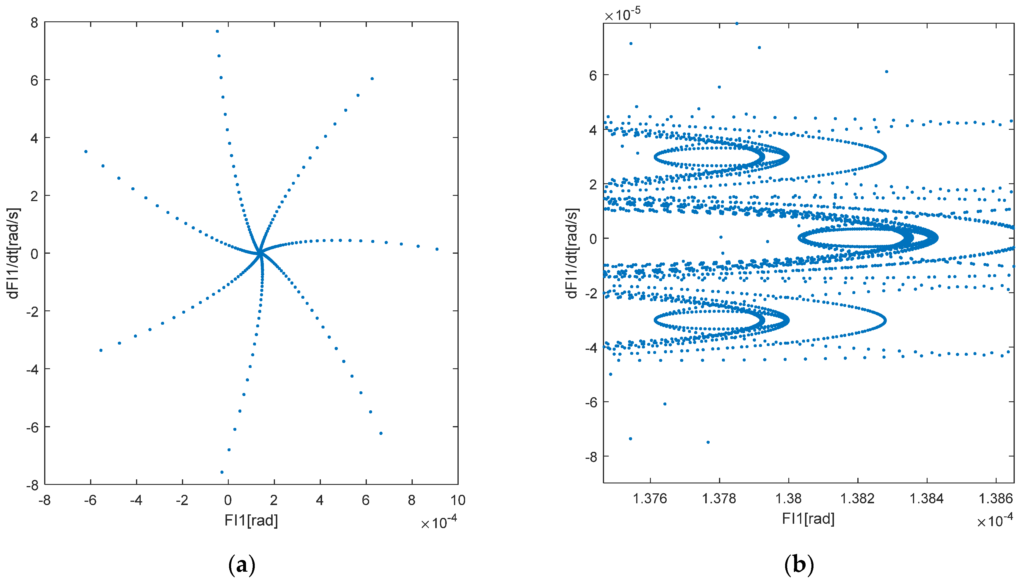
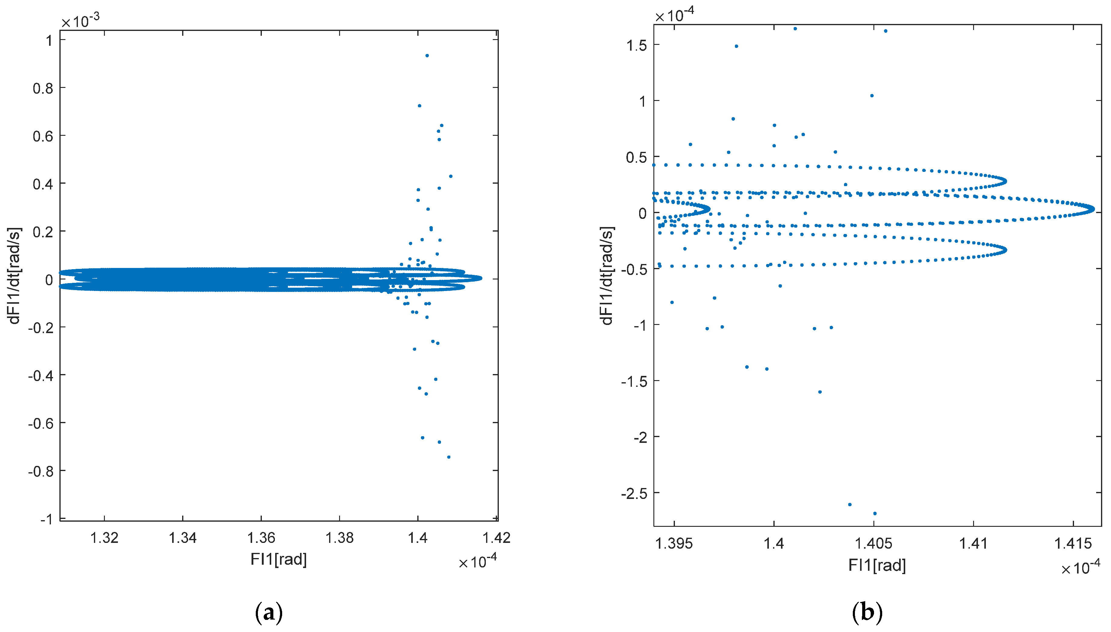
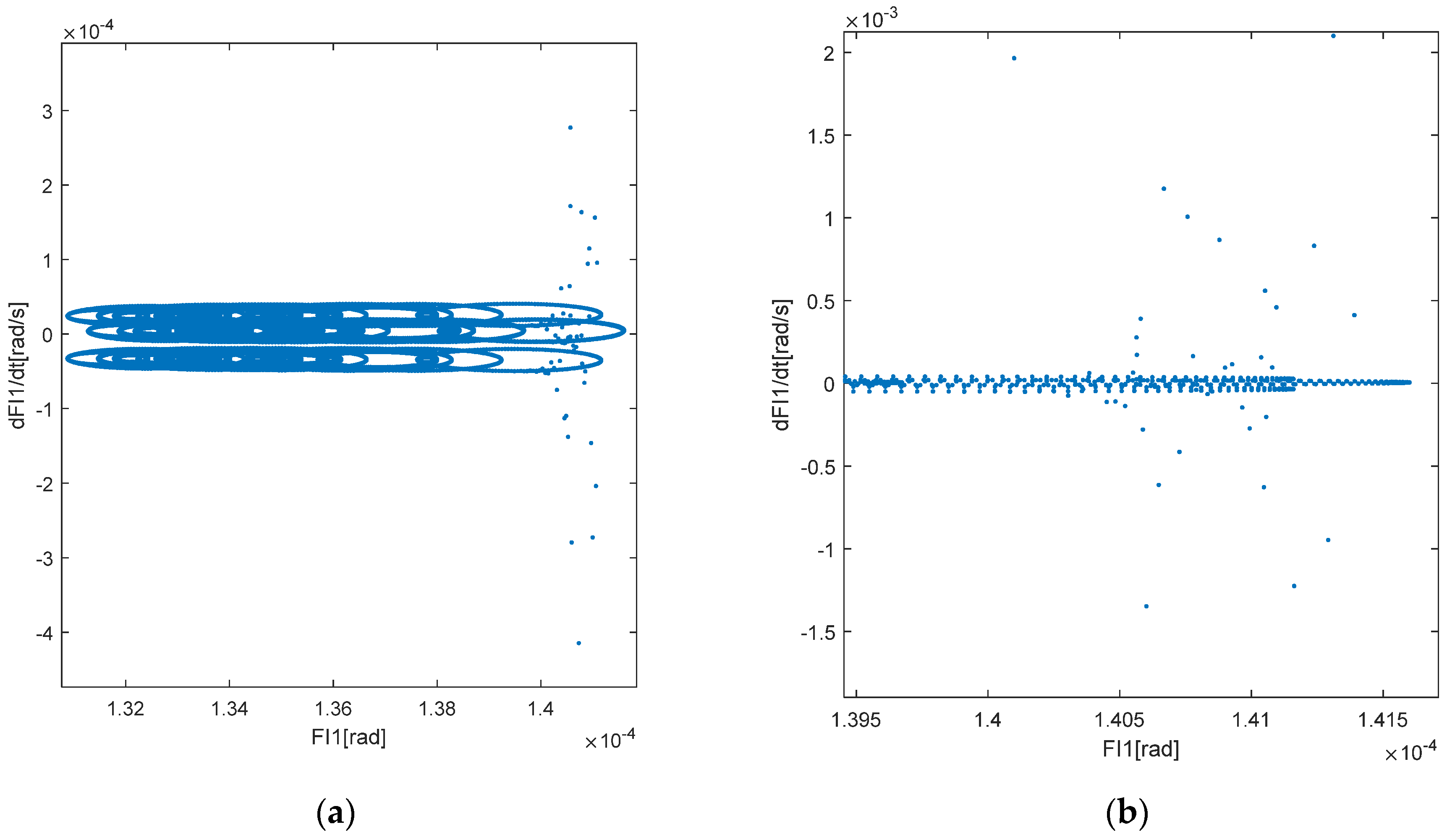
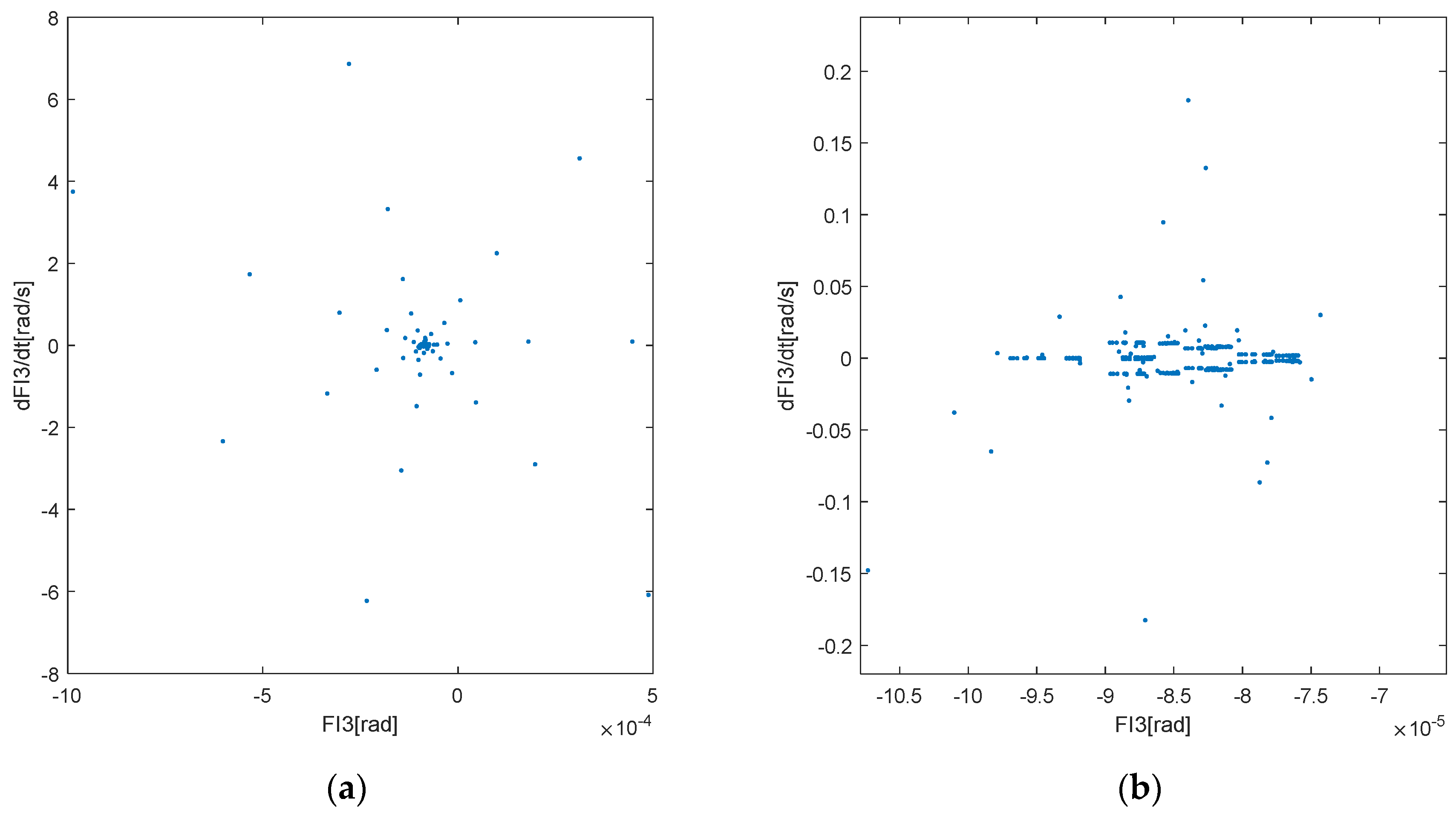
Figure 28, Figure 29 and Figure 30 present the PM for DOE3 when $\mathsf{\xi }=(1.6\dots 10.4)\cdot {10}^{-3},$ ${\mathsf{\eta }}_3=2792\hspace{0.17em}\mathrm{H}\mathrm{z},$ (see Equation (28), Figure 10, and Table 2) ${\mathsf{\beta }}_2=9^0$ using 50,000 to 5000 sections of orthogonal surface to the orbits in the phase portrait $\left({\mathsf{\phi }}_3,\frac{\mathrm{d}{\mathsf{\phi }}_3}{\mathrm{d}\mathrm{t}}\right).$

The pictures illustrated in Figure 28, Figure 29 and Figure 30 demonstrate the properties of PM in the case of the strange attractor: diffuse structure of points having a different density of pixels per unit area of the surface and auto-similarity of the image. For N = 50,000, it is obvious the similarity between the strange attractor of the chaotic dynamic behavior of DIE1 and DOE3, but for $\mathrm{N}\le 15,000$, differences can be noted. In the same way as DIE1 for $\mathsf{\xi }=0.011$, DOE3 has a semblance of chaotic dynamic behavior for $\mathsf{\xi }=0.0104$. A comparison of the images presented in Figure 28 with those illustrated in Figure 30 demonstrate that the strange attractor started to vanish because we are close to the condition $\mathsf{\xi }=11\cdot {10}^{-3}$ when it was manifested in the ergodic dynamic process of DOE3 (see Figure 24). This is the value of the damping ratio starting from which the dynamic behavior of DOE3 becomes an ergodic process. The pictures illustrated in Figure 28, Figure 29 and Figure 30 represent the final confirmation for the occurrence of deterministic chaos (strange attractor) (see Figure 21, Figure 22 and Figure 23) for the NFTV of DOE3 in PPRR for ${\mathsf{\beta }}_2=9^0,{\mathsf{\eta }}_1=2792\hspace{0.17em}\mathrm{H}\mathrm{z}$ and damping ratio in the range $\mathsf{\xi }=(1.6\dots 10.4)\cdot {10}^{-3}$. This may explain the experimental data mentioned by Steinwede in [18] (pp. 88–94), where pitting and microcracks occurred on the interior side of the bels for the DIE1 and DOE3, respectively, as well as manifestations of cracks on the trunnion tripod axes. Steinwede explains these phenomena by the approach of the dynamic behavior in forced torsional vibrations of automotive driveshafts to the dynamic behavior of feared systems. These phenomena appear because of chaotic dynamic behavior, as mentioned in [19,23]. In [19] (p. 104), pitting is due to chaotic dynamic behavior, while the cracks and microcracks result from ergodic dynamic processes for the geared systems. A similar mechanism of inducing such phenomena is manifested for the NFTV of DTID. For a similar dynamic system, the double u-joint driveshaft, Yao and DeSmidt investigated [41] the nonlinear coupled torsional and lateral vibration and the Sommerfeld behavior using the THA. The Sommerfeld effect is a nonlinear phenomenon observed in some rotor systems being driven through a resonance regime when there is not enough power to accelerate the rotor through resonance. Yao and DeSmidt found that this phenomenon is a function of driveline misalignment. Awrejcewicz and Ludwicki [42] investigated the dynamics of a similar system that is the spatial (3D) physical pendulums with nonautonomous systems universal joints. To analyze the dynamic behavior of such a system, Awrejcewicz and Ludwick used THA and the Poincaré Map Method. The novelty of the methods detailed in the present work is detecting chaotic dynamic behavior for NFTV of DTID using THA coupled with the robust method LEA–PM that certifies the deterministic chaos. These new methods must be a part of the design systems of DTID to prevent excessive pitting, microcracks, or even failure as a result of cracks for DTID. The dynamic instability investigation demonstrates that the increase of the damping ratio has a benefic effect. Still, this aspect induces thermo-stress concentrators. Therefore, the growth of the damping ratio of the material for DTID involves the unique design of cooling mechanisms for DTID, engaging chemical composition for the greases used. The new robust THA–LEA–PM method allows the investigation of chaotic manifestation for NFTV of the DTID and has two significant steps, one for detecting chaos manifestation and the second for certifying the deterministic chaos (strange attractor occurrence). For the first step, the THA (based on Equations (25) and (26)) is used while for the second step LEA–PM (based on the four criteria that embed the conditions (37)–(39) and PM) is used. Another novelty of the method is the modification of MLEM (see [23,31]), transforming it into LEA (based on conditions (37)–(39)) and coupling it with PM. This new robust method to investigate the chaos manifestation for NFTV of DTID in PPRR can be named THA–LEA–PM.

7. Conclusions

This study deals with the dynamic instability analysis for the DTID in transition through PPRR. To achieve the goals, an existent model for FTV of AD was modified by designing an MPCM for FTV of a DTID that included the nonuniformity of AGMI, the nonuniformity of AMMI (new aspects of the nonuniformities of AGMI and AMMI for DTID’s elements that were considered till now linked through CVJ, see Appendix A Equations (A1)–(A12)), the quasi-homokinetic TJs of the DTID (new aspects, see Equations (1) and (5)), the external harmonic excitations induced by the asynchronous electric motor (new aspects considering higher-order components of the nonuniformity of the torque load, see Equations (6) and (7)) and the nonuniformity of the reactive torque of the milling system(new aspects considering higher-order components of the nonuniformity of the reactive torque, see Equations (8) and (9)). For the investigation of nonstationary dynamic instability of FTV for DTID’s elements in the PPRR, the THA was designed for the detection of chaotic dynamic behavior based on the Equations (25) and (26), generating the phase portraits that represent the detection of possible chaos manifestation through PPRR of the DTID’s elements. Based on THA, the chaos manifestation for DIE1 was detected through the phase portraits when ${\mathsf{\beta }}_1=9^0$, the damping ratio was in the vicinity range $\mathsf{\xi }\in [1.6,7.3]\cdot {10}^{-3}$ in the PPRR the excitation frequency being in the vicinity of the value ${\mathsf{\eta }}_1\approx 3066\hspace{0.17em}\mathrm{H}\mathrm{z}$ (see Figure 11d and Figure 12d), while for ${\mathsf{\beta }}_1=9^0$, and the damping ratio ${\mathsf{\xi }}_{}\rangle 7.3\cdot {10}^{-3}$ the phase portrait indicated a limit cycle (see Figure 13d). Using THA, the chaos manifestation for DOE3 was detected through the phase portraits when ${\mathsf{\beta }}_2=9^0$, the damping ratio was in the vicinity range $\mathsf{\xi }\in [1.6,6.4]\cdot {10}^{-3}$ in the PPRR the excitation frequency being in the vicinity of the value ${\mathsf{\eta }}_3\approx 2792\hspace{0.17em}\mathrm{H}\mathrm{z}$ (see Figure 14d and Figure 15d), while for ${\mathsf{\beta }}_2=9^0$, and the damping ratio ${\mathsf{\xi }}_{}\rangle 6.4\cdot {10}^{-3}$ the phase portrait indicated a limit cycle (see Figure 16d). A crucial contribution was the computation of the ranges of the principal parametric resonances that vary with the misalignment angles ${\mathsf{\beta }}_1,{\mathsf{\beta }}_2$ and with the nonuniformities of DTID’s AMMIs (see Equations (22) and (23)). Another significant contribution of this study is the development of a new robust method to certify and confirm the deterministic chaos, namely LEA–PM (see the DSOE (29) and (30)). The Lyapunov exponents were computed using Equations (31)–(33) for DIE1 (see Figure 17, Figure 18, Figure 19 and Figure 20) and Equations (34)–(36) for DOE3 (see Figure 21, Figure 22, Figure 23 and Figure 24) and were verified by the conditions (37)–(39) of LEA. Using LEA for DIE1 when ${\mathsf{\beta }}_1=9^0$, the damping ratio is in the vicinity range $\mathsf{\xi }\in [1.6,11.0]\cdot {10}^{-3}$, and the frequency’s excitation is in the range $\left[2950,3200\right]\mathrm{H}\mathrm{z}$ the nonstationary FTV is chaotic (see Figure 17, Figure 18 and Figure 19). Using, for DOE3, LEA when ${\mathsf{\beta }}_2=9^0$, the damping ratio is in the vicinity range $\mathsf{\xi }\in [1.6,6.4]\cdot {10}^{-3}$ and the frequency’s excitation is in the range $\left[2650,2950\right]\mathrm{H}\mathrm{z}$ the nonstationary FTV is chaotic (see Figure 21 and Figure 22). The same manifestation is obtained for DOE3 when ${\mathsf{\beta }}_2=9^0$, the damping ratio is in the vicinity range $\mathsf{\xi }\in [6.4,10.4]\cdot {10}^{-3}$ but the frequency’s excitation is in the range $\left[2700,2925\right]\mathrm{H}\mathrm{z}$, and therefore, the nonstationary FTV is chaotic (see Figure 23).The images determined using the Poincaré Map method for NFTV of DIE1 (see Figure 25, Figure 26 and Figure 27) and DOE3 (see Figure 28, Figure 29 and Figure 30) reconfirmed the chaos manifestation of the DTID’s elements. From the literature survey [30,31,32,33,34,35,36,37,38,39,40,41,42], it was noted that all the research data are based on one method (THA, MLEM, PMM) or two methods (THA–MLEM, THA–PMM) for analyzing the chaotic dynamic behavior of the systems. For the first time, three methods are used to study the chaotic behavior of the DTID through the PPRR: THA for detection of the chaos, LEA (a modified MLEM) to certify the existence of deterministic chaos (strange attractors), and PM to reconfirm deterministic chaos.

The innovations and contributions of the present work can be summarized as follows:

1.

The design of a modified physically consistent model (MPCM) of the FTV for a double tripod industrial driveshaft (DTID) considering the following phenomena:

–

the nonuniformity of axial mass moments of inertia (AMMI) and axial geometric moments of inertia (AGMI) of the DTID’s elements: driving input element 1 (DIE1) and driven output element 3 (DOE3),

–

the geometric inertia nonuniformity of the tripod joints (TJ1 and TJ2) of the DTID,

–

the geometric and kinematic nonuniformity of the quasi-constant velocity joints (quasi-CVJ),

–

the nonuniformity of the torque load’s higher order received by DTID from the asynchronous electric motor,

–

the nonuniformity of the reactive torque’s higher order of the milling system;

2.

The computation of the free natural frequencies of the DTID’s elements as functions of the misalignment angles of the DTID’s elements ${\mathsf{\beta }}_1,{\mathsf{\beta }}_2$, the AMMI and the AGMI of the DTID’s elements;

3.

The use of time–history analysis (THA-phase portraits) to detect the chaotic manifestation of nonstationary FTV for DTID’s elements in transition through principal parametric resonance region (PPRR);

4.

The design of a quantitative method to certify the occurrence of deterministic chaos (strange attractors) LEA (Lyapunov exponents approach), that is a modified MLEM (maximal Lyapunov exponent method) coupled with a new criterion, the sum of all Lyapunov’s exponents is negative, for the nonstationary FTV for DTID’s elements in transition through principal parametric resonance region (PPRR);

5.

The use of Poincaré Maps (PM) to reconfirm the occurrence of deterministic chaos (strange attractors) for the nonstationary FTV for DTID’s elements in transition through principal parametric resonance region (PPRR);

6.

The determination of the range for damping ratio, using THA–LEA–PM, where the deterministic chaos occurs (strange attractor) for the nonstationary FTV for DTID’s DIE1 in transition through principal parametric resonance region (PPRR) ${\mathsf{\eta }}_1\in [2950,3200]\hspace{0.17em}\mathrm{H}\mathrm{z}$ and worst misalignment ${\mathsf{\beta }}_1=9^0$, respectively $\mathsf{\xi }\in [1.6,11]\cdot {10}^{-3}$;

7.

The determination of the range for damping ratio, using THA–LEA–PM, where the deterministic chaos occurs for the nonstationary FTV for DTID’s DOE3 in transition through principal parametric resonance region (PPRR) ${\mathsf{\eta }}_3\in [2700,2925]\hspace{0.17em}\mathrm{H}\mathrm{z}$ and worst misalignment ${\mathsf{\beta }}_2=9^0$, $\mathsf{\xi }\in [1.6,10.4]\cdot {10}^{-3}$;

8.

For the first time, through the chaotic dynamic behavior for the nonstationary FTV for DTID’s elements in transition through the principal parametric resonance region (PPRR), it was revealed theoretically the manifestation of pitting, microcracks, and cracks and the similarity between the phenomena of homokinetic transmission with the phenomena of geared systems transmission.

In conclusion, the robust method THA–LEA–PM, along with the advantages highlighted earlier, also has the considerable advantage of being “mathematical affordable” for designers. This advantage results from the fact that the investigation is possible in the simplest Riemannian space (the space the Euclidian metric), while the newest method of investigating the chaos KCC method, as mentioned in [24], allows this investigation in Finsler spaces (involving the problem of curvature properties of homogeneous Finsler spaces with $\left(\alpha ,\mathsf{\beta }\right)$-metrics which is one of the central problems in Riemann–Finsler geometry) as well as the management of Jacobi stability analysis for Berwald curvature. In the DTID’s design stage, this new robust method THA–LEA–PM prevents the excessive pitting, microcracks, or even failure by cracks for DTID’s elements DIE1, DOE3, and trunnion tripods axes of the DTID’s joints. Future research will enhance the investigation of chaotic dynamic instability of DTID’s NFTV in transition through superharmonic resonances, subharmonic resonances, combination resonances, and internal resonances.