Statistical Characterization of Stress Concentrations along Butt Joint Weld Seams Using Deep Neural Networks

Abstract

In order to ensure high weld qualities and structural integrity of engineering structures, it is crucial to detect areas of high stress concentrations along weld seams. Traditional inspection methods rely on visual inspection and manual weld geometry measurements. Recent advances in the field of automated measurement techniques allow virtually unrestricted numbers of inspections by laser measurements of weld profiles; however, in order to compare weld qualities of different welding processes and manufacturers, a deeper understanding of statistical distributions of stress concentrations along weld seams is required. Hence, this study presents an approach to statistically characterize different types of butt joint weld seams. For this purpose, an artificial neural network is created from 945 finite element simulations to determine stress concentration factors at butt joints. Besides higher quality of predictions compared to empirical estimation functions, the new approach can directly be applied to all types welded structures, including arc- and laser-welded butt joints, and coupled with all types of 3D-measurement devices. Furthermore, sheet thickness ranging from 1 mm to 100 mm can be assessed.

1. Introduction

In welded joints, cracks typically initiate either at imperfections or local stress concentrations. Thus, the fatigue strength and structural integrity is directly linked to the magnitude of distribution of stress concentrations along the seam of welds. In order to improve weld quality by in-production comparisons, it is important to be able to detect and characterize local stress concentrations. In recent years, significant advances have been achieved in the field of automated weld geometry measurements techniques to replace traditional manual weld inspections. In the past, the results of weld inspections were directly linked to the qualification of the performing person [1], which makes unbiased comparisons between different inspections basically impossible. In addition, manual weld inspections are very time consuming and are often performed only on single sections and not on the complete welded joint.

Recent advances in automated measurement techniques allow virtually unrestricted numbers of inspections by optical 3D-measurements of weld profiles. Such measurements are typically based on the digitized surfaces of welds; however, further steps are required to allow comparisons of weld qualities of different welding processes and manufacturers. This includes (i) the development of tools to determine weld geometries from digitalized weld surfaces quickly and reliably, (ii) methods to transfer weld geometries into indicators that describe the local stress concentration or notch effect of welded joints, (iii) the establishment of the relation between these quantities and actual fatigue strength, and (iv) the verification and testing of the developed tools [2]. One important step in this context is a deeper understanding of statistical distributions of weld geometry parameters and stress concentrations along weld seams to use these methods in a reliable and fast manner. Thus, this study presents an approach to statistically characterize different types of butt joint weld seams. For this purpose, an Artificial Neural Network (ANN) is created from 945 finite element simulations to determine Stress Concentration Factors (SCFs) at arc- and laser-welded butt joints with sheet thickness ranging from 1 mm to 100 mm.

Following this introduction, this study is organized as follows. In Section 2, the state of the art on characterization of weld geometries and stress concentrations is introduced. Section 3 describes the finite element modelling and the sampling strategy to determine SCF at butt joint weld seams. The generation of the deep neural network—including the architecture and the training—is described in Section 4. A statistical characterization of weld geometries and stress concentrations along butt joint weld seams made by different welding processes is given in Section 5. Finally, the main findings of this study are discussed in Section 6.

2. State of the Art on Characterization of Weld Geometries and Stress Concentrations

2.1. Characterization of Weld Geometries

To this day, non-destructive testing of engineering structures is, to a large extent, focused on weld defect detection [3]. In addition, visual inspections are performed to ensure sufficient weld quality in accordance with standards such as ISO 5817:2014 [4], Volvo STD 181-0001 [5], or ISO/TS 20273 [6]; however, the extent of such investigations varies and is directly linked to the qualification and training of the person performing the tests. It is thus not surprising that the weld quality of different workshops varies significantly, even if the same preliminary welding procedure specification was applied [7]. Recent developments for both measurement systems and post-processing routines present new possibilities to perform automatic inline quality inspections and thereby fatigue strength assessment of welded joints [2].

Standards to relate the fatigue strength of welded joints to measured geometrical features have existed for several years, e.g., [8,9]; however, these standards are based on numerical calculations rather than measurements and detailed descriptions of weld geometries, c.f., [10,11]. Nevertheless, they provide a suitable tool for a quick quality assessment based on manually measured geometries; yet, for automatic inline quality inspections, the relation between fatigue strength and geometrical parameters needs to be investigated. Hence, the understanding of the statistical variation of weld geometries are crucial to set up computer-aided measurement methods for welded joints. To date, these methods are usually based on 2D profiles of the weld [12].

Weld toe geometries typically vary significantly along weld seams [13]. Thus, the optimal number of measurements per length (also called slices) has to be determined, see [14]. On the other hand, a large number of slices increases processing times, which should preferably be limited. In two recent studies, Renken et al. [15] and Hultgren et al. [16] investigated the effect of sampling rates on measured weld geometries; however, this leads to questions regarding the applicability of current weld quality standards, as the proposed resolution is significantly larger than the resolution of manual measurements. These standards are based on the idea of a few manual gauge measurements. Hence, new methods are required to describe weld qualities. These could, for example, be based on statistical distributions of weld geometry parameters, such as the IBESS procedure [17], and SCFs.

2.2. Characterization of Stress Concentrations along Weld Seams

Besides the fast development of weld geometry measurement systems and algorithms to post-process the measured data, the characterization of stress concentrations at welded joints has also seen significant progress, and it was shown that fatigue cracks often initiate at locations with high stress concentrations [14,16,18].

In the past, parametric SCF equations offered a quick estimation tool to determine SCFs for notched structures such as welded joints [19]; however, a number of recent studies have shown that these equations are less accurate than direct finite element (FE) calculations, see [20,21,22,23,24]. Performing direct FE calculations is, however, quite time consuming, especially for 3D weld geometries. Thus, fitting complex functions to the data provides a fast and reliable way to determine SCFs at welded joints. Various researchers proposed polynomial regression with coupling terms (PRC) and ANN for this task, see [23,24,25,26,27]. By performing several thousand parametric FE simulations, they showed that SCFs can be determined accurately and fast. In addition, their solutions significantly exceed the parameter range of parametric SCF formulas.

Data-driven methods (i.e., machine learning) are increasingly used to predict fatigue of components and parts [28]. Machine learning using ANN is the most common approach [29] and is suitable when large, complex data sets are available and there is no accurate physical description of the phenomenon [30,31,32].

In terms of computational efficiency, ANN, once trained, are superior to other computer-based methods such as FE simulations [29]; however, ANN have very limited ability to make predictions outside the training data space [33,34,35]. In addition, “overfitting” of data can prove problematic, resulting in large deviations when predicting on new data points [33]. A common problem for machine learning algorithm is that the noise or random fluctuations in the training dataset are picked up and memorized as concepts by the model.

By combining advanced tools to determine weld geometry parameters and tools to determine SCFs, it is possible to quickly calculate the change of SCFs along weld seams and to perform inline quality and fatigue strength assessments. For this purpose, a basis for comparison is required to relate measurements to.

To this day, there are only a few studies that consider distributions of weld geometries or stress concentration factors [12,13,16,36,37,38,39,40,41,42,43]; however, there is no thorough investigation of what type of distribution type is suitable for the different geometry parameters and SCFs. Thus, a better understanding of statistical distributions of weld geometry parameters and stress concentrations is needed; nevertheless, first reliable tools to determine stress concentration factors are required. Below, a method to determine stress concentration factors at seam welds of butt joints based on a machine learning approach is presented. This method is then applied to determine statistical distributions of weld geometry parameters and SCFs of weld seams of butt joints made by different welding methods.

3. Finite Element Modeling and Parametrization

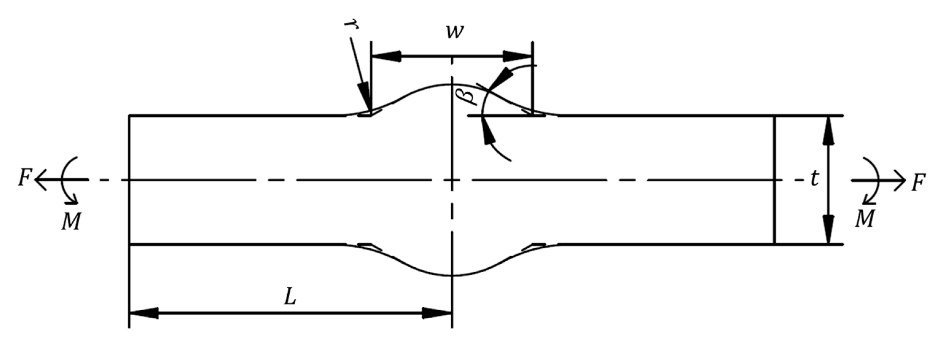
3.1. Geometry of the Butt Joint

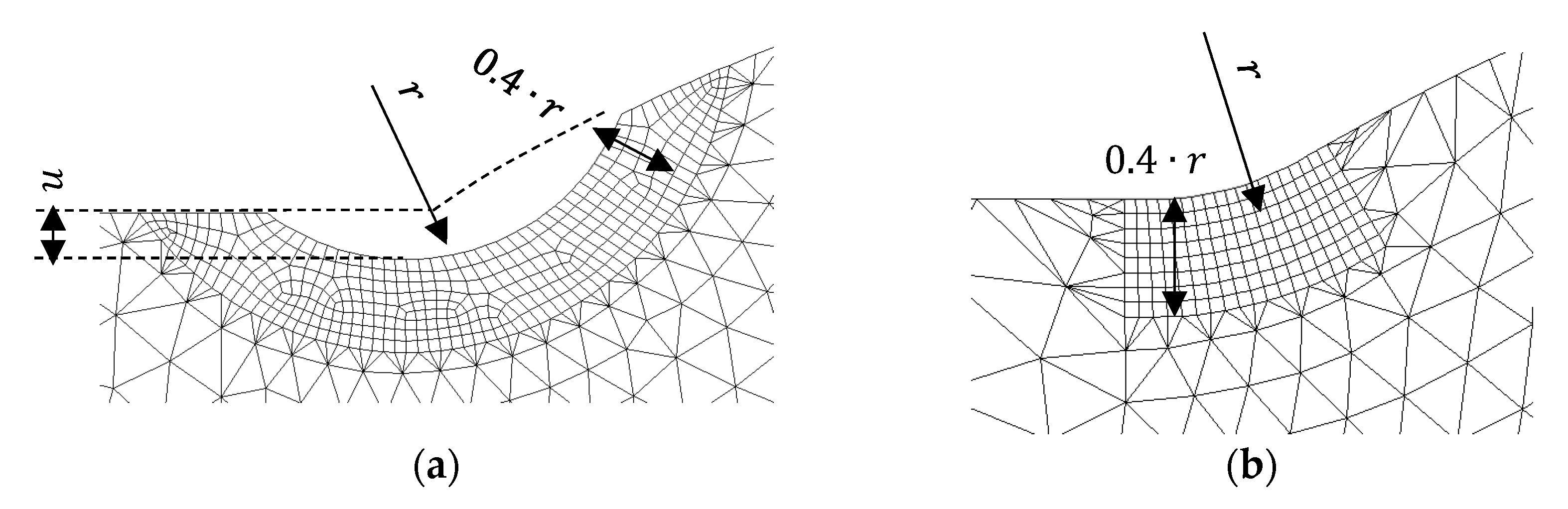
A schematical representation of the butt joint geometry is given in Figure 1. The butt joint is defined by five parameters: the plate thickness t, the weld toe angle β, the weld toe radius r, the ratio of weld seam width to plate thickness w/t, and the undercut u. These parameters are known to be primarily decisive for the SCFs at weld transitions [19,44,45,46] and will therefore be used as input parameter for the machine learning approach based on a neural network. By using a neural network, it is possible to determine SCFs at weld transitions directly from measured weld geometry data without the need for further finite element simulations.

Figure 1 displays the exact definitions of the parameters except for the undercut. The undercut is set in Figure 2.

The geometry parameters are varied within the minimum and maximum bounds of each parameter given in

Table 1. Parameter ranges of the Finite Element Models.

Parameter	Symbol	[Lower Bound/Upper Bound]	Unit
Plate thickness	t	[1/100]	[mm]
Weld toe angle	β	[5/80]	[°]
Weld toe radius	r	[0.05/5]	[mm]
Weld seam width to plate thickness ratio	$\frac{w}{t}$	[0.2/4]	[−]
Undercut depth	u	[0/1]	[mm]

, which were determined by laser measurements. A 3D laser scanner with a spatial resolution of about 0.11 mm and a vertical accuracy of 0.01 mm, attached to a carriage on a stiff frame, were used for the measurements [15]. The lower and upper bound is based on reasonable ranges for these parameters and the resolution of the laser scanning device.

3.2. Discretization

Finite element modeling, meshing, and solving has been performed using ANSYS^® Mechanical^TM 18.1. The finite element models of the butt joint with different parameter combinations have been meshed with quadratic PLANE183 elements with plane strain condition. A preliminary convergence study showed that an adequate resolution of notch stresses is achieved with element edge lengths of 0.05 · r in the notch region. This is five times finer than typical recommendations for notch stress approaches (0.25 · r), see [47,48,49,50].

The mesh is additionally refined perpendicular to the notch radius line up to a depth of 0.4 · r. Exemplary meshes in the notch region are given in Figure 2a in case of the existence of an undercut u > 0 and in Figure 2b in case of the absence of an undercut u = 0.

A global rougher element edge length of 0.05 · t is applied outside of the refined mesh. A complete finite element mesh of one specific design alternative with an undercut depth u > 0 is given in Figure 3.

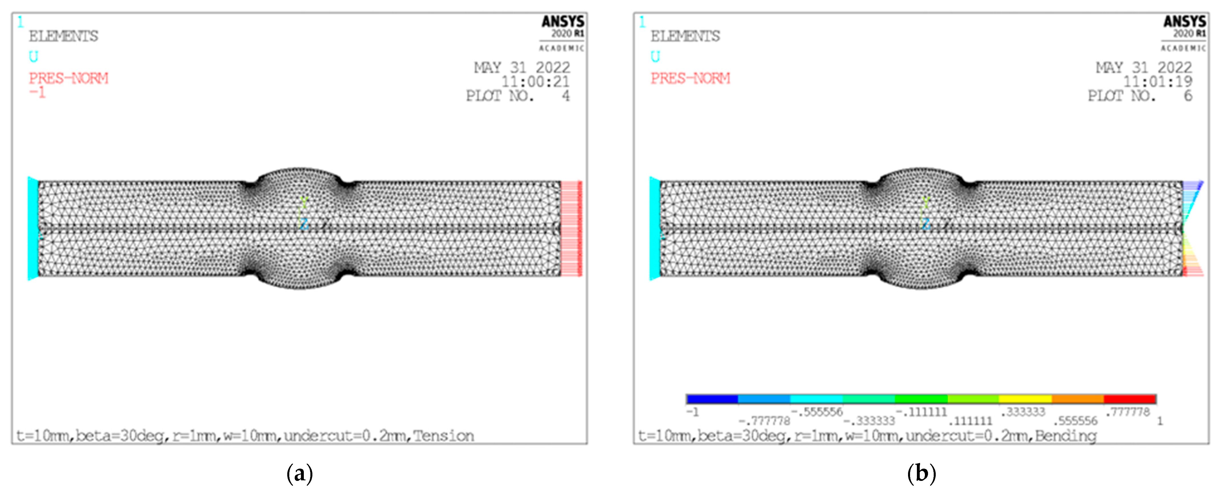
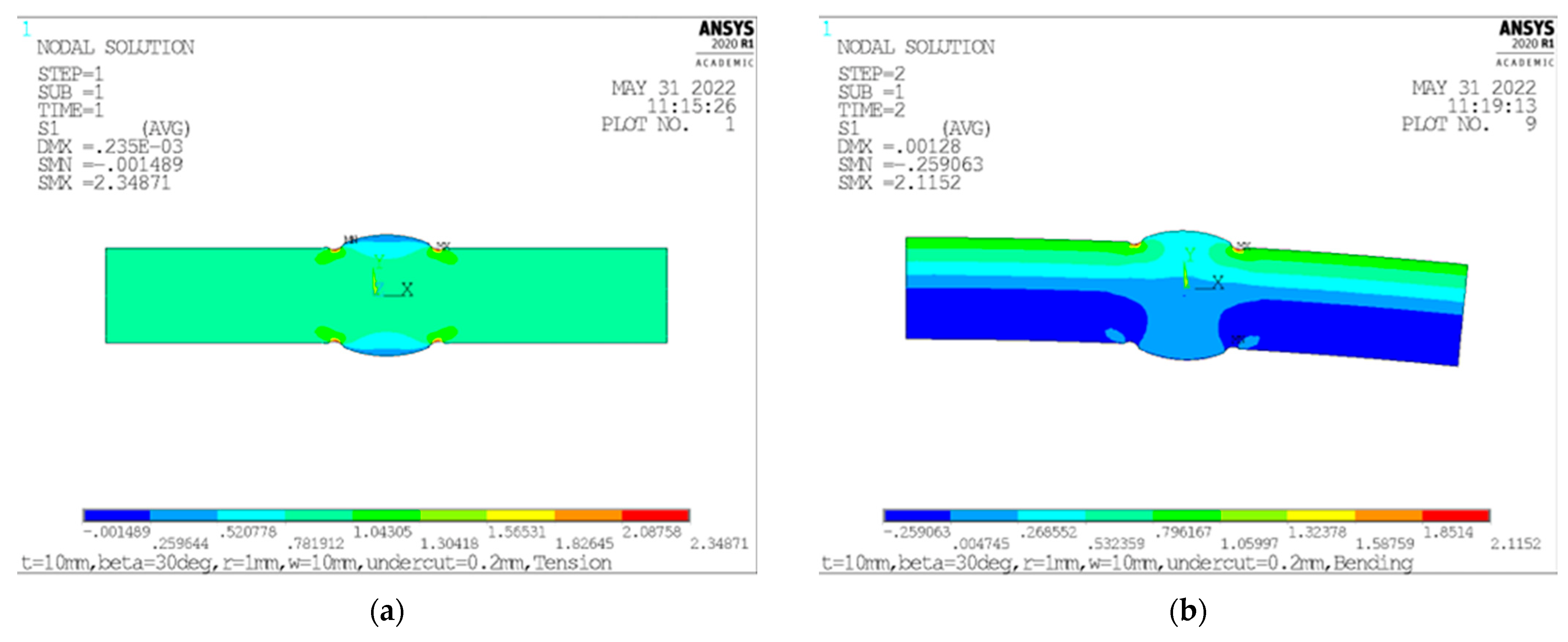
3.3. Load Cases and Solution

Besides the finite element meshes, Figure 3 also shows the load case definition. Unit tension and bending stresses of 1 MPa are defined for the two load cases. The purely linear-elastic solutions for the butt joint in Figure 3 exposed to tension and bending loading are illustrated in Figure 4.

The averaged nodal stress plots for the solution of the butt joint configuration of Figure 3 are shown in Figure 4. As pre-defined nominal tension and bending stresses of 1 MPa are used, the resulting notch stress in form of the maximum principal stress is evaluated and will furthermore be described as the Stress Concentration Factor for tension (SCF_t) and for bending (SCF_b).

3.4. Sampling Strategy

The regression analysis with neural networks requires many data points. These data points are generated within the design space with the lower and upper parameter bounds in Table 1. The software optiSLang^® 8.0.0 was used for the purpose of design of experiments as the software provides many different sampling strategies. The Advanced Latin Hypercube Sampling provides 1000 samples. These 1000 samples were assumed to be a sufficient baseline for the discretization of the design space. Each sample represents one specific combination of geometry parameters.

After sampling, the parameter combinations are sent to the ANSYS solving process. The input geometry parameters and the output Stress Concentration Factors SCF_t and SCF_b are stored for training of the neural network.

4. Generation of the Deep Neural Network

As it is impractical to perform an FE simulation for each combination of weld geometry parameters, a Deep Neural Network (DNN) is established to ease the calculation of SCFs. A DNN is a subtype of an ANN with several layers.

The regression of the FEM data is performed using Keras 2.4.0, which is a powerful deep learning framework that can be accessed with Python. The resulting DNN helps to predict data points that were not used for the training of the neural network. This section aims to explain the individual steps and measures of the generation of the DNN which had to be taken to ascertain a sufficient accuracy of untrained predicted samples.

In the context of ANN, the geometry parameters will be referred to as features and the Stress Concentration Factors SCF_t and SCF_b as labels which is motivated by Raschka and Mirjalili [51].

4.1. Restrictions of the FEM Data

The initial 1000 samples are reduced to 945 samples because:

• In 36 cases, finite element models could not be generated due to irrational combinations of geometry parameters.
• A further 19 calculated samples were excluded due to extreme parameter combinations. The parameter combinations lead to SCF > 6 and resulted, for example, from the combination of a high plate thickness t, a high weld toe angle β, a small weld toe radius r, and a high ratio of weld seam width to plate thickness w/t.

As a result of these restrictions, the proposed deep neural network is only applicable for butt welds with SCF ≤ 6. Other studies used even more strict requirements, see, e.g., Alam et al. [13].

4.2. Preprocessing of the FEM

Before the training of the deep neural network, the FEM data was split into training data, validation data, and test data. The test data, 20% of the 945 samples, were randomly chosen and exclusively used for testing the DNN. Additionally, 30% of the remaining data were excluded from training, which are called validation data. During training, loss and model metrics are evaluated for the validation and training data which helps to avoid overfitting of the DNN.

One way to ensure a proper convergence of the training is to normalize features as they have different scales and ranges of validity. Therefore, mean and variance (var) of the features/inputs are computed and the inputs are normalized:

$$\frac{input-mean}{sqrt\left(var\right)}$$

(1)

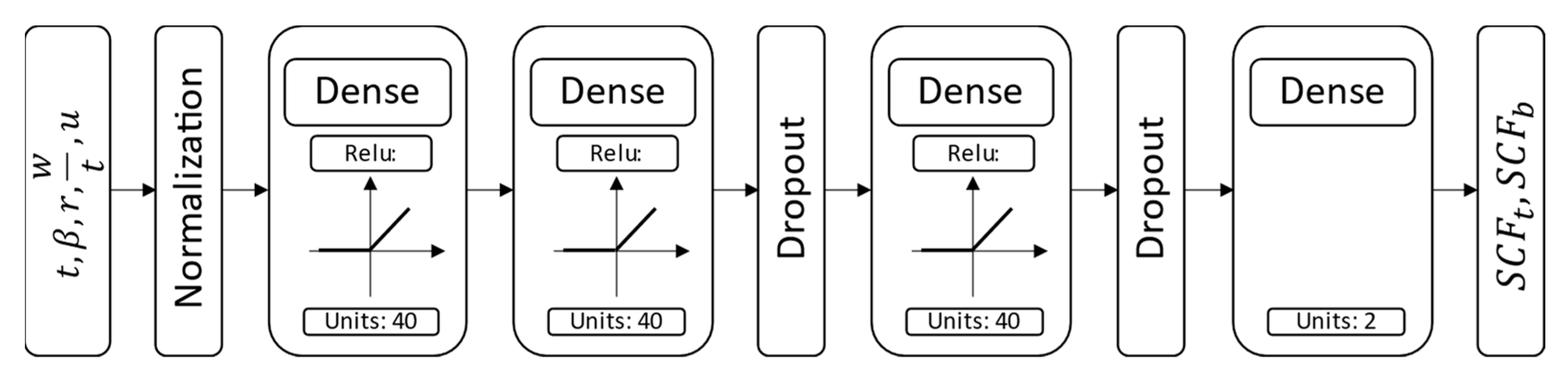
4.3. Architecture of the DNN

The DNN consists of one normalization layer, three non-linear hidden layers with 40 units and the rectified linear unit (relu) activation function. The final output layer yields two outputs, SCF_t and SCF_b. One specific method to prevent neural networks from overfitting is dropout [52]. Dropout with a tunable hyperparameter p = 0.1 was applied after the second and third hidden layers and thins out units from the hidden layers with a given probability. The architecture of the DNN is visualized in Figure 5.

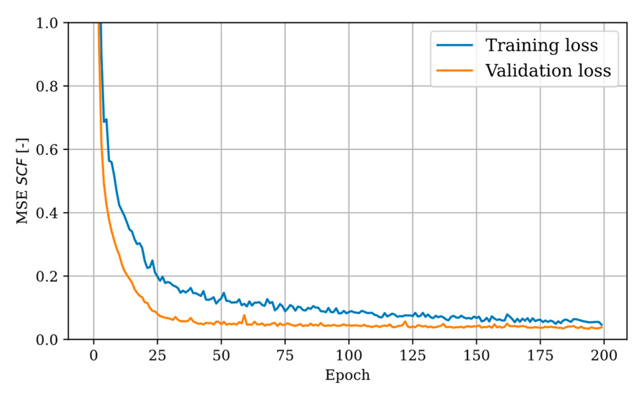
4.4. Training of the DNN

The neural network is trained with a stochastic optimizer called Adam [53] that requires only first-order gradients and thus is computationally efficient. Mean squared error (MSE) is defined to be the loss. Training is carried out for 200 epochs. The training history is shown in Figure 6. The validation loss in terms of MSE is slightly below training loss throughout the entire training history, which is due to the use of dropout. The curves of training loss and validation loss converge towards a common value. Further training did not affect the steady state value that both curves reached after 200 epochs of training.

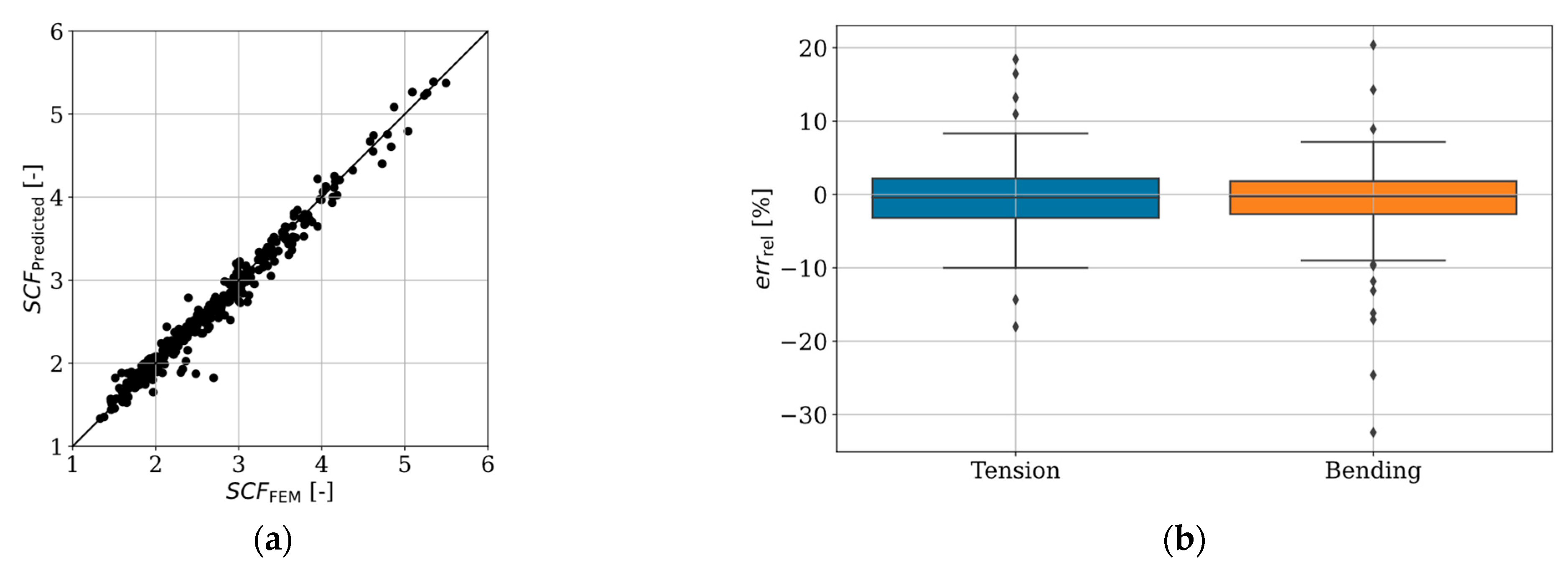
4.5. Performance of the DNN

The data points in Figure 7a,b solely represent the test data set which consists of data points that have not been used for the training the DNN. These samples have been predicted by the neural network and are compared to the exact known values from FEA in two different ways.

Figure 7a shows predicted SCFs for bending and tension versus exact SCFs by FEA. In cases in which a sample was perfectly predicted by the neural network, the data point would lie on the diagonal black line.

Figure 7b shows relative errors of the predicted SCFs to the exact SCFs by FEA in the form of two box plots, each boxplot for either tension or bending loading. The relative errors are calculated by:

$${err}_{\mathrm{rel}}=\frac{{SCF}_{\mathrm{Predicted}}-{SCF}_{\mathrm{FEM}}}{{SCF}_{\mathrm{FEM}}}·100 [\%]$$

(2)

The middle line within the boxes shows the median value of the relative errors, while the box around this line includes 50% of the data from the 25% to the 75% percentile. The black whiskers outside of the box extend to 1.5 of the interquartile range. The remaining outliers outside of the whiskers are beyond this level.

5. Statistical Characterization of Weld Geometries and Stress Concentrations along Butt Joint Weld Seams

This method is now applied to determine statistical distributions of weld geometry parameters and SCFs of weld seams of butt joints made by different welding methods. To this end, laser scans of butt joints taken from [54,55,56,57,58] and other unpublished investigations were collected and assessed using the weld geometry assessment algorithm presented in Renken et al. [15].

In total, 80 welded plates produced by Submerged Arc Welding (SAW), Flux-Cored Arc Welding (FCAW), laser-, and laser-hybrid welding were measured by a laser scanner to obtain the weld geometry along the weld seam. To simplify sampling and to reduce movement-related vibrations of the scanning setup, segments of about 40 mm length were measured in 0.15 mm steps and later combined to reproduce the weld seam. Figure 8 presents the change of weld geometry parameters and SCFs along an exemplary 36 mm weld segment. In the following sections, only the SCF for tension loading is presented, as the results for the bending SCF are similar.

On the left side of Figure 8, the change of weld geometry parameters along the weld seam obtained using the curvature method [15,59] are presented, as well as the SCF under tension loading based on the DNN presented in Section 4. The determined weld geometry parameters are weld toe radii, weld toe angles, and undercut depths on the left and right side of the weld seam, as well as the weld reinforcement height and width.

On the right side, histograms of the measured parameters are presented, including four statistical measures to describe the distributions. The four measures are kurtosis k, skewness s, median m, and variance v. While the median represents the value for which 50% of the sample are larger and 50% are smaller, the unbiased or empirical sample variance presents a measure for the spread of data:

$$v=\frac{1}{n-1}\sum _{i=1}^n{\left(x_i-\overline{x}\right)}^2$$

(3)

where $\overline{x}$ is the mean of x_i and n the number of observations.

The skewness is a measure of the asymmetry of the data around the sample mean:

$$s=\frac{1}{n}\sum _{i=1}^n{\left(\frac{x_i-\overline{x}}{\sigma }\right)}^3$$

(4)

with σ representing the standard deviation. If the skewness is negative, the data spread to the left, and if the skewness is positive the data spread to the right. The skewness of a symmetrical distribution (e.g., a normal distribution) is zero. Typical distribution functions have a skewness between ±3. Values outside this range are generally considered severely skewed.

The fourth parameter is the kurtosis of a sample:

$$k=\frac{1}{n}\sum _{i=1}^n{\left(\frac{x_i-\overline{x}}{\sigma }\right)}^4$$

(5)

The kurtosis is a measure for how outlier-prone a distribution is. For example, a normal distribution has a kurtosis of k = 3. The higher the kurtosis, the more the data spreads around the mode of a distribution. The variance, skewness, and kurtosis are also known as the second, third, and fourth central moments of a distribution.

Figure 8 shows that, in particular, the kurtosis and skewness vary for the measured geometrical parameters and the SCF. In contrast, the parameters are similar on the left and right side of the weld seam. Interestingly, three parameters are left- and three are right-skewed. From a visual assessment, some histograms could be described by a normal or lognormal distribution; however, even for such a small step size of 0.15 mm, the amount of data is limited and not yet representative for longer weld seams. Thus, in the next step, the data along the full weld seam of about 1 m length are assessed.

Table 2. Skewness and kurtosis of a number of typical distribution functions.

Distribution	Skewness	Kurtosis
Normal	0	3
Exponential	2	9
Lognormal	$\left(e^{{\sigma }^2}+2\right)\sqrt{e^{{\sigma }^2}-1}$	$e^{4{\sigma }^2}+2e^{3{\sigma }^2}+3e^{2{\sigma }^2}-3$
Gamma	$2/\sqrt{\alpha }$	$3+6/\alpha$
Inverse gamma	$\frac{4\sqrt{\alpha -2}}{\alpha -3}$ for α > 3	$\frac{6(5\alpha -11)}{\left(\alpha -3\right)\left(\alpha -4\right)}+3$ for α > 3

presents the skewness and kurtosis of different typical two-parameter distribution functions that are compared to the investigated parameters. In this table, σ and α are the shape parameters of the Lognormal, Gamma, and Inverse Gamma distributions, respectively.

In Figure 9, exemplary histograms for three welding methods are shown, as it would be impossible to directly compare the change of weld parameters along the weld seam. Again, differences between weld parameters are clearly visible. In addition, differences between the welding methods become obvious. This supports findings by Schubnell et al. [12], who presented a comparison of distributions for weld toe radii and flank angles obtained from literature.

Interestingly, while, for example, the histogram for the weld toe angle of the flux-cored arc welded plate is only slightly skewed, see Figure 9b, and somewhat resembles a normal distribution, the histograms of the other two plates, see Figure 9a,b, are significantly more skewed. Thus, below, the measured sample parameters are used next to determine whether the weld parameters can be described by well-known distribution functions. To this end, a skewness–kurtosis plot is created to compare these two important features of the measured samples with theoretical distributions, see Figure 10. As reference, the distributions presented in Table 2 are used. As skewness values may be either positive or negative, the square of skewness is typically used in such plots.

The typical range for such a plot is s² < 4 and k < 9; nevertheless, in some cases, data falls outside this range, see [60]. In fact, for every weld parameter, a number of measures for the different plates fall outside this range. Thus, the range was increased to accommodate data that is only slightly outside this range; however, there are still a number of measurements that are outside this range. This might be related to a number of reasons, which are subsequently discussed, but first the main observations based on Figure 10 are listed:

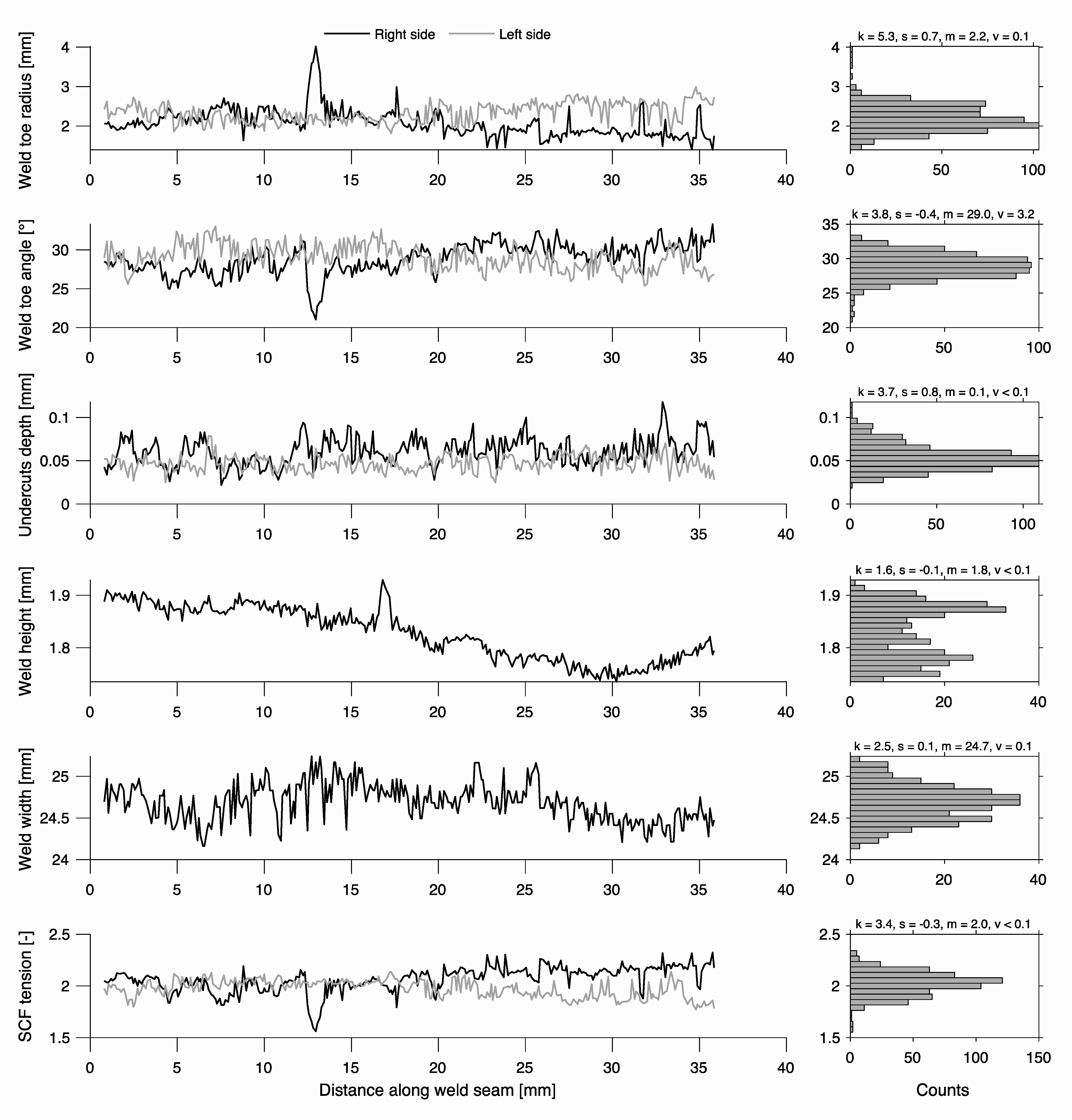
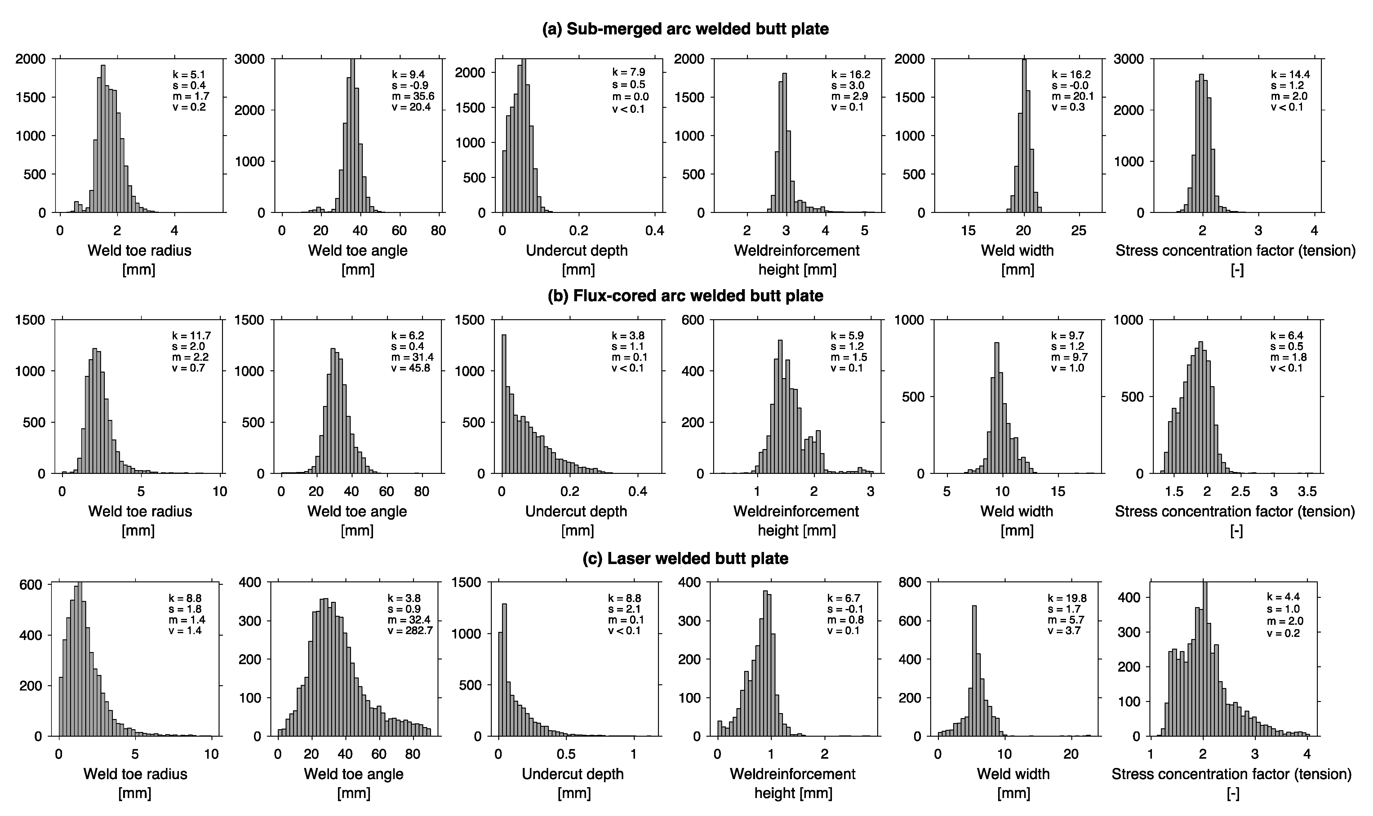
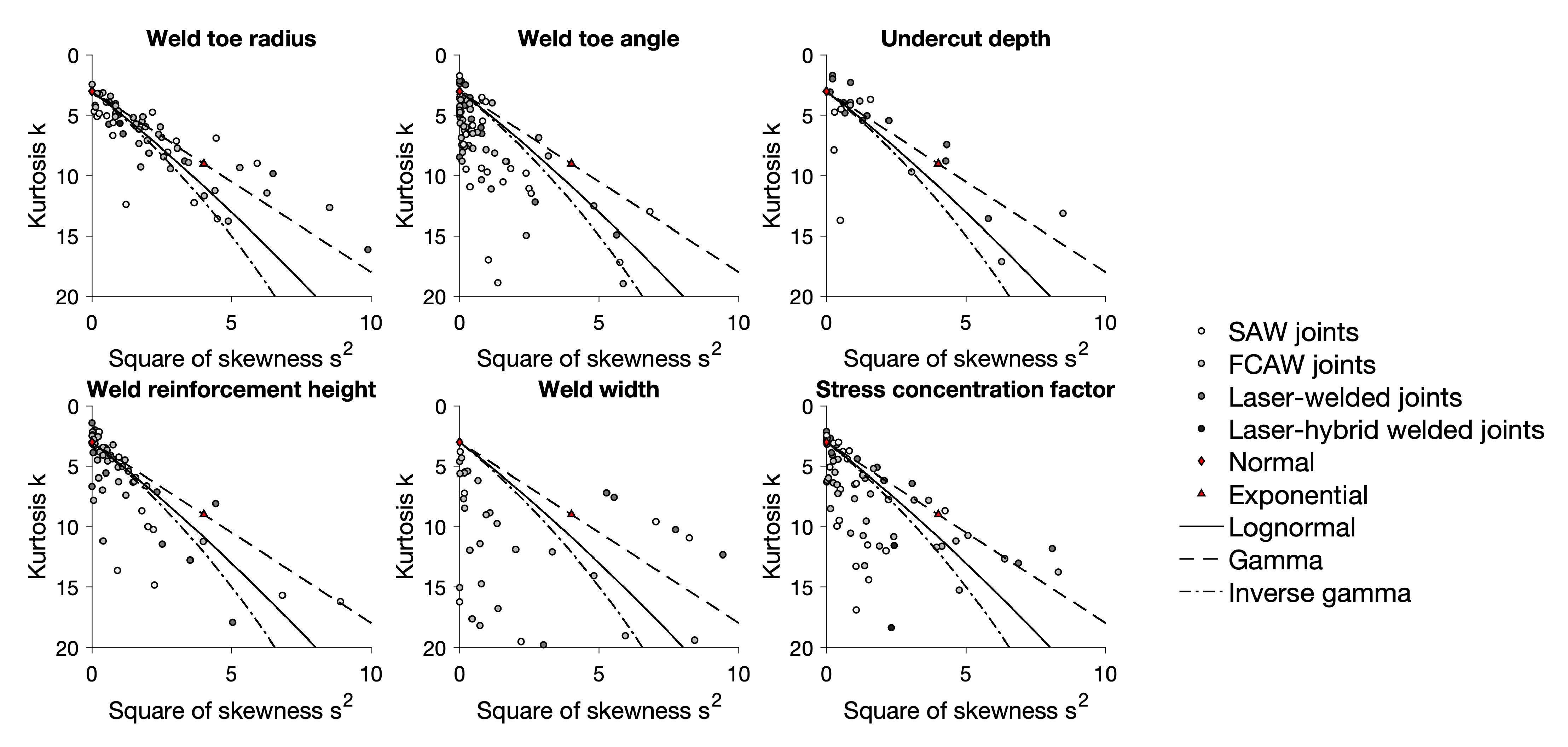
• The measured sample skewness and kurtosis of the weld toe radii is close to the line representing the lognormal, the gamma, and the inverse gamma distribution. Interestingly, the weld toe radii also show, on average, the smallest scatter of kurtosis.
• The majority of plates have weld toe angles with distributions that are only slightly skewed. This is an indication for a symmetrical distribution such as a normal distribution; nevertheless, the partially high kurtosis indicates that the tails of the distributions are wider than typical for a normal distribution.
• The distributions of undercuts are the most skewed; 70% of the skewness–kurtosis combinations are outside the range plotted in Figure 10. The reason is that very small shape parameters α are required to fit distributions as presented in Figure 9, which increases the skewness and kurtosis; nevertheless, the data are close to the dashed line in and outside the presented range, which represents parameter combinations of a gamma distribution.
• The data for the weld reinforcement heights are clustered around the normal distribution and the region where lognormal, gamma, and inverse gamma distribution are close to each other.
• Except for the weld toe angles and weld reinforcement heights, the majority of datasets have sample kurtosis k ≫ 3 and square of skewness s² ≫ 0, which suggests that a normal distribution is not suited to describe the data. Similarly, the exponential distribution does not seem to be suitable for any of the assessed parameters and datasets.
• The distributions of weld widths and SCFs show a large scatter. This makes it difficult to relate them to a typical distribution function. Interestingly, the majority of the data on weld width in Figure 10 and thereby in the range of typical less-skewed distribution functions are for plates made by FCAW, which were manually welded. A large fraction of the other joints, which were automatically welded, are outside the range presented in Figure 10.

6. Discussion

6.1. Discussion of the Skewness–Kurtosis Comparison

In general, the comparison of skewness and kurtosis of the measured samples with theoretical distributions showed that it is difficult to determine suitable distribution functions for the investigated weld geometry parameters and SCFs. This might be related to non-stationary processes that result in variations along weld seams but also measurement inaccuracies; however, trends can be discovered and related to other published data.

In the literature [38,39,40,42,43], weld toe radii and angles are sometimes stated to be normally distributed. Here, the weld toe radii seem to be better described by a lognormal distribution. This agrees with a number of recent studies [20,36,37]. As the sample distributions of the measured weld toe angles are symmetrical, it is possible that this parameter is indeed well-described by a normal distribution; however, more data should be assessed to verify this result.

Undercuts can be considered a type of weld defect; thus, gamma distributions might be a suitable choice to describe the depth of undercuts. Gamma distributions are frequently used for such tasks; however, more research is required. Ottersböck et al. [20] and Schork et al. [36,37] used a lognormal distribution to fit their data, which also accommodates very large numbers of small undercut depths; however, a lognormal distribution is not suited to describe distributions for which the maximum of data is equal to zero. In general, data for undercut depths are seldom presented nor considered in the literature. It is therefore not yet possible to come to a conclusion.

Based on Figure 10, weld reinforcement heights could either be normally distributed or described by a lognormal, gamma, or inverse gamma distribution. In the literature, the height of welds is often described by a normal distribution [20,36,37,43].

Finding suitable distributions for the weld width and SCFs is difficult. Interestingly, the data for the automatically welded joints made by SAW, laser- and laser-hybrid welding is heavily skewed and outside the range presented in Figure 10. This could be related to the fact that the welder is able to manually adjust the welding process, while the automatic process is not able to do so. The constant heat-input with the inhomogeneous heat distribution in the plates might lead to a change in weld gap and thereby to a drift in weld width. The drift in weld width was confirmed by assessing the change of parameters along the weld seam for several segments.

The reason for the scatter of the sample parameters of the SCFs might be related to the fact that the SCF calculation is based on the input of a number of geometrical features. Thus, the variability and any possible inaccuracy in the input parameters is transferred to the SCFs. As the MSE of the DNN is almost zero, inaccuracies of the DNN can be ruled out as long as the measured parameter are within the parameter range used to train the DNN. This was ensured by filtering measured parameters outside the training range; however, only a small amount of measured data was removed this way.

Finally, the combination of various parameters might also be the reason why typical two-parameter distribution functions are not suitable to describe a complex parameter such as a SCF. Clearly, more data and research on the variability of this parameter are required to establish a better understanding of the variability of SCFs along weld seams.

6.2. Discussion of the Applicability Readiness of the Presented Methodology

Numerous studies have shown a significant influence of local weld geometry on the fatigue strength or life of welded joints [10,11,36,38,40]. In welded structures, the weld transition acts as a local stress raiser that can cause fatigue cracks, which often initiate at locations with high stress concentrations [14,16,18]. Hence, a representative quantity for the influence of the notch effect at the seam transition is the SCF [19].

The weld toe radius, the weld angle [44,45,46], and the depth of undercuts [19] are primarily decisive for the SCFs at weld transitions. In the past, SCFs were mainly determined by parametric estimation functions that were computed with FE simulations; however, those simulations were limited due to the required computational methods of the time. Nowadays, it is much easier to perform a few thousand FE simulations and to train a neural network on the data, which also provides a higher accuracy. In the current study, a high accuracy of the neural network was ensured by performing a sensitivity analysis and a mesh refinement five times smaller than typical recommendations for notch stress approaches, which yields a deviation from the converged stresses of less than 1%.

Data-driven methods are increasingly used to predict fatigue of components and parts [28] but also to determine SCFs. In terms of computational efficiency, ANN, once trained, are clearly superior to other computer-based methods such as FE simulations [29]; however, ANN have very limited ability to make predictions outside the training data space [33,34,35]. This also applies to DNNs as a subtype of ANNs. Thus, a wide range of meaningful parameter combinations was selected to train the DNN of this study.

ANN and DNN are now an established method to determine SCFs and might be suitable for automatic inline quality inspections and to assess the relation between fatigue strength and geometrical features. To achieve this goal, a number of steps have to be taken. The research of the last years has primarily focused on two of the aforementioned points: (i) the development of tools to determine weld geometries reliably and fast digitalization of weld surfaces and (ii) methods to transfer weld geometries into indicators that describe the notch effect and fatigue performance of welded joints. Thus, two major points remain to be solved to use the presented methodology in design: (iii) the relation between these quantities and actual fatigue strength has to be established and (iv) the developed tools have to be tested and verified [2].

7. Summary and Conclusions

One important step in this context is a deeper understanding of statistical distributions of weld geometry parameters and stress concentrations along weld seams. This study presents an approach to statistically characterize different types of butt joint weld seams made by different welding methods. For this purpose, an artificial neural network was created from thousands of finite element simulations to determine SCFs at arc- and laser-welded butt joints with sheet thickness ranging from 1 mm to 100 mm.

The following conclusions are drawn from the statistical characterization of weld geometry parameters and stress concentrations along butt joint weld seams using deep neural networks:

• Establishing a DNN for a recurring task such as the determination of SCFs at weld transition significantly decreases the required time to determine the severity of notches along weld seams by combining the mutual influence of stress-raising effects from local weld geometry factors such as weld toe radii, angles, and undercuts.
• The comparison of skewness and kurtosis of the measured samples with theoretical distributions showed that it is difficult to determine suitable distribution functions for the investigated weld geometry parameters and SCFs. This might be related to non-stationary processes that result in variations along weld seams (e.g., due to inhomogeneous temperature fields) but also measurement inaccuracies. Modelling inaccuracies are mitigated by using highly refined FE meshes to calculate the input data for the DNN.
• Weld toe radii seem to follow a lognormal distribution. This agrees with a number of recent studies [20,36,37], but also rejects mainly older investigations.
• The majority of weld toe angle sample distributions are only slightly skewed. This is an indication for a symmetrical distribution like a normal distribution; nevertheless, the partially high kurtosis indicates that the tails of the distributions are wider (more outlier-prone) than typical for a normal distribution.
• The distributions of undercuts are the most skewed. The reason is that very small shape parameters α are required to fit distributions as presented in Figure 9, which increases the skewness and kurtosis; nevertheless, the data is close to a gamma distribution. A gamma distribution might be better suited to describe undercut depths (for which the maximum of data is equal to zero) as a lognormal distribution.
• The data for the weld reinforcement heights are clustered around the normal distribution and the region where lognormal, gamma, and inverse gamma distribution are close to each other.
• The distributions of weld widths and SCFs show a large scatter. This makes it difficult to relate them to a typical distribution function. The reason for the scatter of the sample parameters of the SCFs might be related to the fact that the SCF calculation is based on the input of a number of geometrical features. Thus, the variability and any possible inaccuracy in the input parameters and numerical modelling is transferred to the SCFs. In addition, the combination of various parameters could be the reason typical two-parameter distribution functions are not suitable to describe a complex parameter such as a SCF.

In summary, this study presents promising results, but more data should be assessed to verify the result of this study and in order to establish a basis for automatic inline quality inspections of welded joints beyond the scope of current manual weld inspections after welding.

References

1. Hammersberg, P.; Olsson, H. Statistical evaluation of welding quality in production. In Proceedings of the Swedish Conference on Light Weight Optimized Welded Structures, Borlänge, Sweden, 24–25 March 2010; pp. 148–162. [Google Scholar]
2. Braun, M. Recent progress on geometrical and stress concentration characterization of welded joints. In Proceedings of the 7th International E-Conference on Industrial, Mechanical, Electrical, and Chemical Engineering (ICIMECE 2021), Virtual, 5 October 2021. [Google Scholar]
3. Amirafshari, P.; Barltrop, N.; Wright, M.; Kolios, A. Weld defect frequency, size statistics and probabilistic models for ship structures. Int. J. Fatigue 2021, 145, 106069. [Google Scholar] [CrossRef]
4. EN ISO 5817:2014; Welding—Fusion welded joints in steel, nickel, titanium and their alloys (beam welding excluded)—Quality levels for imperfections. European Committee for Standardization: Brussels, Belgium, 2014.
5. STD 181-0001; Volvo welding standard. Volvo Group: Gothenburg, Sweden, 2014.
6. ISO/TS 20273:2017-08; Guidelines on weld quality in relationship to fatigue strength. European Committee for Standardization: Brussels, Belgium, 2017.
7. Öberg, A.E.; Åstrand, E. Variation in welding procedure specification approach and its effect on productivity. Procedia Manuf. 2018, 25, 412–417. [Google Scholar] [CrossRef]
8. Hobbacher, A.F.; Kassner, M. On Relation Between Fatigue Properties Of Welded Joints, Quality Criteria and Groups in Iso 5817. Weld. World 2013, 56, 153–169. [Google Scholar] [CrossRef]
9. Jonsson, B.; Dobmann, G.; Hobbacher, A.F.; Kassner, M.; Marquis, G.B. IIW Guidelines on Weld Quality in Relationship to Fatigue Strength; Springer: Berlin/Heidelberg, Germany, 2016. [Google Scholar] [CrossRef]
10. Jonsson, B.; Samuelsson, J.; Marquis, G.B. Development of Weld Quality Criteria Based on Fatigue Performance. Weld. World 2013, 55, 79–88. [Google Scholar] [CrossRef]
11. Åstrand, E.; Stenberg, T.; Jonsson, B.; Barsoum, Z. Welding procedures for fatigue life improvement of the weld toe. Weld. World 2016, 60, 573–580. [Google Scholar] [CrossRef]
12. Schubnell, J.; Jung, M.; Le, C.H.; Farajian, M.; Braun, M.; Ehlers, S.; Fricke, W.; Garcia, M.; Nussbaumer, A.; Baumgartner, J. Influence of the optical measurement technique and evaluation approach on the determination of local weld geometry parameters for different weld types. Weld. World 2020, 64, 301–316. [Google Scholar] [CrossRef]
13. Alam, M.M.; Barsoum, Z.; Jonsen, P.; Kaplan, A.F.H.; Häggblad, H.Å. The influence of surface geometry and topography on the fatigue cracking behaviour of laser hybrid welded eccentric fillet joints. Appl. Surf. Sci. 2010, 256, 1936–1945. [Google Scholar] [CrossRef]
14. Hultgren, G.; Barsoum, Z. Fatigue assessment in welded joints based on geometrical variations measured by laser scanning. Weld. World 2020, 64, 1825–1831. [Google Scholar] [CrossRef]
15. Renken, F.; von Bock und Polach, R.U.F.; Schubnell, J.; Jung, M.; Oswald, M.; Rother, K.; Ehlers, S.; Braun, M. An algorithm for statistical evaluation of weld toe geometries using laser triangulation. Int. J. Fatigue 2021, 149, 106293. [Google Scholar] [CrossRef]
16. Hultgren, G.; Myrén, L.; Barsoum, Z.; Mansour, R. Digital Scanning of Welds and Influence of Sampling Resolution on the Predicted Fatigue Performance: Modelling, Experiment and Simulation. Metals 2021, 11, 822. [Google Scholar] [CrossRef]
17. Zerbst, U.; Madia, M.; Schork, B.; Hensel, J.; Kucharczyk, P.; Ngoula, D.; Tchuindjang, D.; Bernhard, J.; Beckmann, C. Fatigue and Fracture of Weldments; Springer: Berlin/Heidelberg, Germany, 2019. [Google Scholar] [CrossRef]
18. Madia, M.; Zerbst, U.; Beier, H.T.; Schork, B. The IBESS model—Elements, realisation and validation. Eng. Fract. Mech. 2018, 198, 171–208. [Google Scholar] [CrossRef]
19. Haibach, E. Betriebsfestigkeit: Verfahren und Daten zur Bauteilauslegung, 3rd ed.; Springer: Berlin/Heidelberg, Germany, 2006. [Google Scholar]
20. Ottersböck, M.J.; Leitner, M.; Stoschka, M. Characterisation of actual weld geometry and stress concentration of butt welds exhibiting local undercuts. Eng. Struct. 2021, 240, 112266. [Google Scholar] [CrossRef]
21. Wang, Y.; Luo, Y.; Tsutsumi, S. Parametric Formula for Stress Concentration Factor of Fillet Weld Joints with Spline Bead Profile. Materials 2020, 13, 4639. [Google Scholar] [CrossRef]
22. Pachoud, A.J.; Manso, P.A.; Schleiss, A.J. New parametric equations to estimate notch stress concentration factors at butt welded joints modeling the weld profile with splines. Eng. Fail. Anal. 2017, 72, 11–24. [Google Scholar] [CrossRef]
23. Oswald, M.; Mayr, C.; Rother, K. Determination of notch factors for welded cruciform joints based on numerical analysis and metamodeling. Weld. World 2019, 63, 1339–1354. [Google Scholar] [CrossRef]
24. Oswald, M.; Neuhäusler, J.; Rother, K. Determination of notch factors for welded butt joints based on numerical analysis and metamodeling. Weld. World 2020, 64, 2053–2074. [Google Scholar] [CrossRef]
25. Oswald, M.; Springl, S.; Rother, K. Determination of Notch Factors for Welded T-Joints Based on Numerical Analysis and Metamodeling; International Institute of Welding: Paris, France, 2020. [Google Scholar]
26. Neuhäusler, J.; Rother, K. Determination of notch factors for transverse non-load carrying stiffeners based on numerical analysis and metamodeling. Weld. World 2022, 66, 753–766. [Google Scholar] [CrossRef]
27. Dabiri, M.; Ghafouri, M.; Rohani Raftar, H.R.; Björk, T. Utilizing artificial neural networks for stress concentration factor calculation in butt welds. J. Constr. Steel Res. 2017, 138, 488–498. [Google Scholar] [CrossRef]
28. Chen, J.; Liu, Y. Fatigue modeling using neural networks: A comprehensive review. Fatigue Fract. Eng. Mater. Struct. 2022, 45, 945–979. [Google Scholar] [CrossRef]
29. Kalayci, C.B.; Karagoz, S.; Karakas, O. Soft computing methods for fatigue life estimation: A review of the current state and future trends. Fatigue Fract. Eng. Mater. Struct. 2020, 43, 2763–2785. [Google Scholar] [CrossRef]
30. Lee, J.A.; Almond, D.P.; Harris, B. The use of neural networks for the prediction of fatigue lives of composite materials. Compos. Part A-Appl. Sci. Manuf. 1999, 30, 1159–1169. [Google Scholar] [CrossRef]
31. Ross, C.T. Best Practice Guidelines for Developing Neural Computing Applications—An Overview; Ministry of Defense Procurement Executive: London, UK, 1993. [Google Scholar]
32. Uygur, I.; Cicek, A.; Toklu, E.; Kara, R.; Saridemir, S. Fatigue Life Predictions of Metal Matrix Composites Using Artificial Neural Networks. Arch. Metall. Mater. 2014, 59, 97–103. [Google Scholar] [CrossRef] [Green Version]
33. Abambres, M.; Lantsoght, E.O.L. ANN-Based Fatigue Strength of Concrete under Compression. Materials 2019, 12, 3787. [Google Scholar] [CrossRef] [Green Version]
34. Vassilopoulos, A.P.; Bedi, R. Adaptive neuro-fuzzy inference system in modelling fatigue life of multidirectional composite laminates. Comput. Mater. Sci. 2008, 43, 1086–1093. [Google Scholar] [CrossRef]
35. Yang, J.Y.; Kang, G.Z.; Liu, Y.J.; Kan, Q.H. A novel method of multiaxial fatigue life prediction based on deep learning. Int. J. Fatigue 2021, 151, 106356. [Google Scholar] [CrossRef]
36. Schork, B.; Kucharczyk, P.; Madia, M.; Zerbst, U.; Hensel, J.; Bernhard, J.; Tchuindjang, D.; Kaffenberger, M.; Oechsner, M. The effect of the local and global weld geometry as well as material defects on crack initiation and fatigue strength. Eng. Fract. Mech. 2018, 198, 103–122. [Google Scholar] [CrossRef]
37. Schork, B.; Zerbst, U.; Kiyak, Y.; Kaffenberger, M.; Madia, M.; Oechsner, M. Effect of the parameters of weld toe geometry on the FAT class as obtained by means of fracture mechanics-based simulations. Weld. World 2020, 64, 925–936. [Google Scholar] [CrossRef]
38. Lieurade, H.P.; Huther, I.; Lefebvre, F. Effect of Weld Quality and Postweld Improvement Techniques on the Fatigue Resistance of Extra High Strength Steels. Weld. World 2008, 52, 106–115. [Google Scholar] [CrossRef]
39. Stenberg, T.; Lindgren, E.; Barsoum, Z. Development of an algorithm for quality inspection of welded structures. Proc. Inst. Mech. Eng. Part B J. Eng. Manuf. 2012, 226, 1033–1041. [Google Scholar] [CrossRef]
40. Barsoum, Z.; Jonsson, B. Influence of weld quality on the fatigue strength in seam welds. Eng. Fail. Anal. 2011, 18, 971–979. [Google Scholar] [CrossRef]
41. Seshadri, A. Statistical Variation of Weld Profiles and Their Expected Influence on Fatigue Strength. Master’s Thesis, Lappeenrante Univercity of Technology, Lappeenranta, Finland, 2006. [Google Scholar]
42. Harati, E.; Ottosson, M.; Karlsson, L.; Svensson, L.-E. Non-destructive measurement of weld toe radius using Weld Impression Analysis, Laser Scanning Profiling and Structured Light Projection methods. In Proceedings of the First International Conference on Welding and Non Destructive Testing (ICWNDT2014), Islamic Azad University, Karaj Branch-Karaj-Alborz, Iran, 25–26 February 2014; pp. 1–8. [Google Scholar]
43. Remes, H. Strain-Based Approach to Fatigue Strength Assessment of Laser-Welded Joints. Ph.D. Thesis, Helsinki Univercity of Technolgy, Helsinki, Finland, 2008. [Google Scholar]
44. Lassen, T. The Effect of the Welding Process on the Fatigue Crack Growth. Weld. J. 1990, 69, 75–82. [Google Scholar]
45. Nykänen, T.J.; Marquis, G.; Björk, T. Effect of weld geometry on the fatigue strength of fillet welded cruciform joints. In Proceedings of the International Symposium on Integrated Design and Manufacturing of Welded Structures, Eskilstuna, Sweden, 13–14 March 2007. [Google Scholar]
46. Nguyen, T.N.; Wahab, M.A. A Theoretical-Study of the Effect of Weld Geometry Parameters on Fatigue-Crack Propagation Life. Eng. Fract. Mech. 1995, 51, 1–18. [Google Scholar] [CrossRef]
47. Fricke, W. IIW Recommendations for the Fatigue Assessment of Welded Structures by Notch Stress Analysis: IIW-2006-09; Woodhead Publishing: Cambridge, UK, 2012. [Google Scholar]
48. Fricke, W. Round-Robin Study on Stress Analysis for the Effective Notch Stress Approach. Weld. World 2013, 51, 68–79. [Google Scholar] [CrossRef]
49. Baumgartner, J.; Bruder, T. An efficient meshing approach for the calculation of notch stresses. Weld. World 2012, 57, 137–145. [Google Scholar] [CrossRef]
50. Braun, M.; Müller, A.M.; Milaković, A.-S.; Fricke, W.; Ehlers, S. Requirements for stress gradient-based fatigue assessment of notched structures according to theory of critical distance. Fatigue Fract. Eng. Mater. Struct. 2020, 43, 1541–1554. [Google Scholar] [CrossRef]
51. Raschka, S.; Mirjalili, V. Python Machine Learning: Machine Learning and Deep Learning with Python, Scikit-Learn, and TensorFlow 2; Packt Publishing Ltd.: Birmingham, UK, 2019. [Google Scholar]
52. Srivastava, N.; Hinton, G.; Krizhevsky, A.; Sutskever, I.; Salakhutdinov, R. Dropout: A simple way to prevent neural networks from overfitting. J. Mach. Learn. Res. 2014, 15, 1929–1958. [Google Scholar]
53. Kingma, D.P.; Ba, J. Adam: A method for stochastic optimization. arXiv 2014, arXiv:1412.6980. [Google Scholar]
54. Braun, M.; Milaković, A.-S.; Ehlers, S.; Kahl, A.; Willems, T.; Seidel, M.; Fischer, C. Sub-Zero Temperature Fatigue Strength of Butt-Welded Normal and High-Strength Steel Joints for Ships and Offshore Structures in Arctic Regions. In Proceedings of the ASME 2020 39th International Conference on Ocean, Offshore and Arctic Engineering, Fort Lauderdale, FL, USA, 28 June–3 July 2020. [Google Scholar]
55. Braun, M.; Kahl, A.; Willems, T.; Seidel, M.; Fischer, C.; Ehlers, S. Guidance for Material Selection Based on Static and Dynamic Mechanical Properties at Sub-Zero Temperatures. J. Offshore Mech. Arct. Eng. 2021, 143, 1–45. [Google Scholar] [CrossRef]
56. Braun, M.; Kellner, L.; Schreiber, S.; Ehlers, S. Prediction of fatigue failure in small-scale butt-welded joints with explainable machine learning. Procedia Struct. Integr. 2022, 38, 182–191. [Google Scholar] [CrossRef]
57. Braun, M.; Ahola, A.; Milaković, A.-S.; Ehlers, S. Comparison of local fatigue assessment methods for high-quality butt-welded joints made of high-strength steel. Forces Mech. 2021, 6, 100056. [Google Scholar] [CrossRef]
58. Braun, M.; Kellner, L. Comparison of machine learning and stress concentration factors-based fatigue failure prediction in small-scale butt-welded joints. Fatigue Fract. Eng. Mater. Struct. 2022; submitted for publication. [Google Scholar]
59. Jung, M. Development and Implementing an Algorithm for Approximation and Evaluation of Stress Concentration Factors of Fillet Welds Based on Contactless 3D Measurement. Master’s Thesis, Karlsruher Institut für Technologie, Karlsruhe, Germany, 2018. [Google Scholar]
60. Hammond, R.K.; Bickel, J.E. Reexamining Discrete Approximations to Continuous Distributions. Decis. Anal. 2013, 10, 6–25. [Google Scholar] [CrossRef] [Green Version]
Figure 1. Butt joint geometry and loading conditions.
Applsci 12 06089 g001
Figure 2. Notch geometry and mesh refinement at the notch in case of: (a) the existence of an undercut; (b) the absence of an undercut.
Applsci 12 06089 g002
Figure 3. Finite element mesh and applied boundaries for the load case: (a) tension; (b) bending.
Applsci 12 06089 g003
Figure 4. Nodal averaged solution for maximum principal stress for the load case: (a) tension; (b) bending.
Applsci 12 06089 g004
Figure 5. Visualization of the DNN.
Applsci 12 06089 g005
Figure 6. Training history of the DNN.
Applsci 12 06089 g006
Figure 7. Quality of predicted SCFs in the form of: (a) scatter plot; (b) box plot.
Applsci 12 06089 g007
Figure 8. Change of weld geometry parameters and SCFs along exemplary weld seams.
Applsci 12 06089 g008
Figure 9. Exemplary histograms of various important geometrical parameters that describe weld geometries obtained from assessing weld seam sections about 1 m long.
Applsci 12 06089 g009
Figure 10. Skewness–kurtosis plot presenting the determined sample parameters and a number of common two-parameter distribution functions.
Applsci 12 06089 g010